Predicting Critical Problems from Execution Logs of a Large-Scale Software System

Predicting Critical Problems from Execution Logs of a

Large-Scale Software System

´

Arp´ad Besz´edes, Lajos Jen˝o F¨ul¨op and Tibor Gyim´othy Department of Software Engineering, University of Szeged

´

Arp´ad t´er 2., H-6720 Szeged, Hungary

(beszedes|flajos|gyimi)@inf.u-szeged.hu

Abstract. The possibility of automatically predicting runtime failures in large-scale distributed systems such as critical slowdown is highly desirable, since this way a significant amount of manual effort can be saved. Based on the analysis of execution logs, a large amount of information can be gained for the purpose of prediction. Existing approaches – which are often based on achievements in Complex Event Processing – rarely employ intelligent analyses such as machine learning for the prediction. Predictive Analytics on the other hand, deals with ana-lyzing past data in order to predict future events. We have developed a framework for our industrial partner to predict critical failures in their large-scale telecom-munication software system. The framework is based on some existing solutions but include novel techniques as well. In this work, we overview the methods and present initial experimental evaluation.

Keywords

Predictive Analytics, Complex Event Processing, predicting runtime failures, machine learning, execution log processing.

1 Introduction

Modern large-scale software systems are often distributed – composed of several sub-systems, for example, database sub-systems, application servers, and other domain specific layers. Failures occurring during the operation of these systems are many times very difficult to track down due to the complexity and size of the systems. For finding causes of failures, most of the times the administrators or operators of the systems rely on low level monitoring techniques such as monitoring CPU or memory load, disk usage, application load, and so forth. Due to the huge amount of data to be processed and produced in the execution logs, it is almost impossible to monitor such large systems purely manually. So, usually more sophisticated (semi-)automatic analysis methods are applied, such as those belonging toComplex Event Processing(CEP) [1]. CEP tools abstract the low level events into a high level form which is more easier to understand.

However, even with the help of CEP tools, manual monitoring is required (often employing a whole team of administrators), which demands high costs and constant attention. This is because although CEP tools present easily understandable high level

events, the administrators are still responsible to interpret the events to find out whether an alert given by the tools requires any further action. The approaches taken by CEP tools rarely provide more intelligent data analyses that could automatically predict pos-sible problems in the future based on past data. However, the field ofpredictive analyt-ics(PA) perfectly fits to this problem area. PA deals with methods and techniques (such as data mining, statistics, machine learning, etc.) with the aim to forecast future events based on past data. Using PA, the effort to interpret CEP-related results could be greatly reduced.

In this paper, we present our first experiences in applying PA to a set of CEP-related problems in the domain of large-scale distributed telecommunication software. An in-dustrial partner asked us to conduct research in this field and produce tailored methods to forecast runtime problems (such as critical slowdown) in their large-scale telecom-munication software system. We detail on our framework developed for this project, where we reused some existing techniques, but also developed specialized analysis al-gorithms. We experimented with different algorithms with different success rates. The results of initial experiments are presented.

We will proceed as follows. In Section 2, we will present the prediction framework. Afterwards, in Section 3, we will describe our experiments. In the following section, we will discuss some works that are similar to ours. Finally, we will close our paper with conclusions and directions for future work in Section 5.

2 Framework

The development of the prediction framework is motivated by forecasting concrete problemsoccurring in large-scale telecommunication software of an industrial partner. We could have applied existing solutions, but the input given by the industrial partner was too special. Furthermore, introducing an existing solution, like a CEP technique would require too much costs and resources from our industrial partner. These facts motivated us to develop a new framework and not to use an existing one. We apply existing components like Weka [2], but not complete solutions.

In the paper, the large-scale telecommunication software will be referred to as sub-ject system. After several discussions with the industrial partnertwo eventshave been selected as the object of the prediction. The first one is theprediction of changes in file systems, and the other one is thedirect prediction of the concrete problems; both occurred in the subject system. The latter is based on the idea, that some attribute of the system that normally change together suddenly does not, which can be a potential pre-dictor of a concrete problem. After all, both events can be considered as the prediction of the problems. The only difference between them is that theprediction of changes in file systemsis an indirect method: it is based on the fact that the changes could imply that some kind of problem is arising.

First, a brief description of the required concepts is given, and afterwards the ar-chitecture of the prediction framework is shown. Finally, datatransformation methods will be detailed. As we will show it, these data transformation methods were the major supporters of the prediction of the previously mentionedtwo events.

2.1 Definitions

In this subsection, we define some required concepts. The following machine learn-ing [3] concepts will occur several times in the paper:

– Machine learning algorithmscan predict future events on present data by using previously observed data and previously known events. In other wordsmachine learning algorithmstry to learn a function, or try to build a model, which maps input data (predictors) into an event.

– We worked withdiscrete functionswhere the predictions were different events, for example, whether problems occurred or not (problemevent andno problemevent). This is usually calledclassification.

– In thelearning phase, the machine learning algorithm got thepredictorsand the eventsas well. In this phase, the learning algorithm built a modelbased on the relationships of thepredictorsand theevents.

– In thetesting phase, the machine learning algorithm got onlythe predictor values and the previously determinedmodelto predict thefuture event.

After the basic concepts we need to introduce another one as follows. If we have a dataset which covers a certain time interval, and we have certain number of events on this interval, how can we run a machine learning algorithm and how can we test the produced model? A trivial solution would be that we split the time interval into a learning part and a testing part. The learning part should be used during the learning phase, while the testing part should be used in the testing phase. However, in the case the results are really dependent on the circumstances of the experiment.

Another solution is where the whole data is split intoxparts and the learning-testing phases are runxtimes. In each learning-testing phase, we run the learning on the union ofx-1parts, and we run the test on the remaining part. This techniques is known in the literature as thefold cross validation[4], and most of the times ten-fold cross validation is applied (x=10).

2.2 Architecture

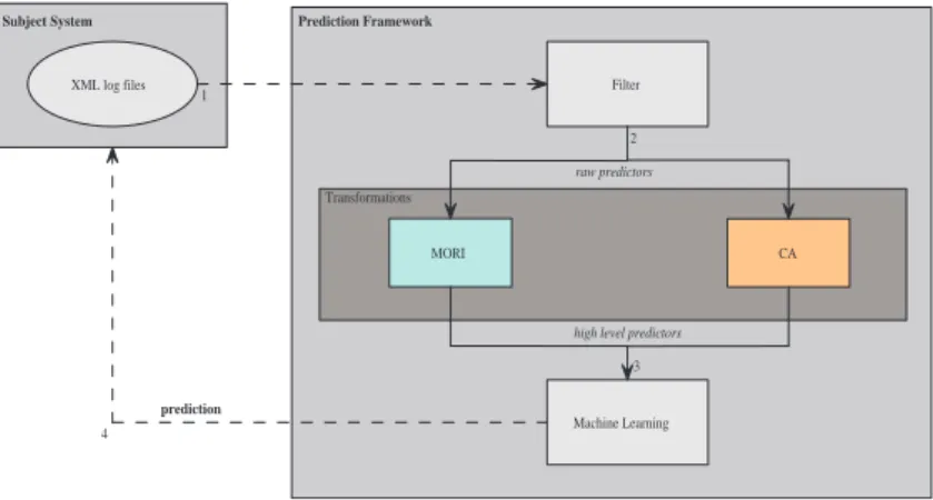
Figure 1 represents the architecture of theprediction framework. The basic process is the following.

Filtering. The Subject Systemhas a logging subsystem which produces its results in XML log files. The first step of theprediction frameworkis extracting the relevant in-formation from these XML files. The XML files store fragments of log files made by different programs and the results of scripts querying different kinds of system infor-mation. A significant part of the information stored in the files is not relevant, so we have developed a general method for filtering out the relevantpredictors. The filtering is completely general; filtering further predictors can be easily implemented by a plug-in mechanism. In filterplug-ing, it is important to considertime, which means that the data are filtered for a certain time interval (e.g. for a day, for an hour, etc.). Thistimefactor is also a parameter of the framework. This way, several experiments can be made to find the best parameters.

Transformations. In the second step, certain transformations are performed on the pre-dictors produced byfiltering. The filtered butraw predictorsare too simple for a ma-chine learning algorithm. We found out that the transformation of theraw predictors intohigh level predictorscan improve the prediction abilities of machine learning al-gorithms. We developed several data transformation methods and chose the best two methods to be published. One of them is theMaximum Of Relative Increasing(MORI) data transformation method, which can be applied for simplifying linear predictors. The other one is theCorrelation Anomalies(CA) data transformation, which can be applied for predictor pairs. The data transformation methods will be detailed in subsection 2.3.

Subject System XML log files Prediction Framework Filter MORI Transformations Machine Learning

high level predictors

prediction 1 2 CA 3 4 raw predictors

Fig. 1.Architecture of the prediction framework

Machine learning In the third step, machine learning methods are applied. We ran the machine learning algorithms by using the high level predictorsproduced by the data transformation methods. Several variants of machine learning algorithms are known, for example, decision trees [5], neural networks [6], or genetic algorithms [7]. By using machine learning algorithms different kinds of problems can be solved, for example, re-gression or classification problems. Theprediction frameworkuses only classification tasks. We applied two decision tree based algorithms from Weka [2], J4.8 (Java imple-mentation of C4.5 [8]) and Logistic Model Tree [9]. The Logistic Model Tree algorithm differs from a usual decision tree because its leaves represent logistic regression func-tions instead of classification labels.

Prediction. In the current work, we just implemented theFilteringandTransformations phases, and appliedMachine Learningalgorithms. Now, during theMachine Learning phase we applycross-fold validationtechniques for testing the models (please see Sec-tion 2.1 for definiSec-tions). The fourth step of theprediction frameworkwill be a future work. In the future, it will be possible to integrate the models produced by the machine learning methods into theSubject System.

2.3 Data transformation methods

In this Section, we present the two data transformation methods we have developed during this work. Sometimes, in the paper we refer to the whole process – filtering, transforming and learning – with the name of the data transformation method, because it is the key sub process of the whole prediction framework.

Maximum Of Relative Increasing – MORI. At the beginning of this work we tried to predict problems in a special way. With the help ofSubject Systemprofessionals, we started out from the fact that the fullness of file systems can be the cause of serious problems. Therefore, we tried to predict this event, but we faced a problem. No exam-ple existed where a file system was full. To resolve this problem, wetransformedthe data in a way that the machine learning algorithms had to learn the changes of a given file system. The prediction of changes is another important piece of information, for example, when the fullness of a file system is 90%, the prediction that it will increase by more than 12% on the following day is very beneficial.

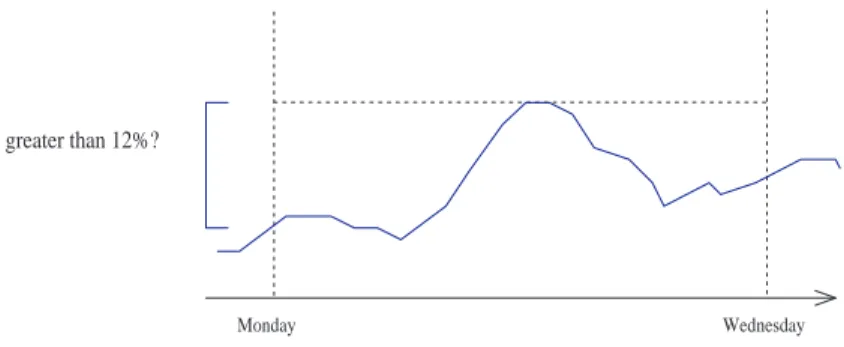
To predict the changes in file systems, we have developed theMaximum Of Relative Increasing(MORI) method. The name of this method implies that for a given interval, the maximum of relative increase will be greater than a bound. During this method, machine learning produces a model which helps us predict whether there will be a change above the bound or not for a givenptime frame. For example, ifpis 2 days between Monday and Wednesday, and the bound is 12%, then the model tells us whether or not there will be an increase above 12% in the following two days (compared to the beginning time point, see Figure 2). The method has another parameter for refreshing the prediction. For example, if it is set at one hour, it gives a new prediction in every hour. MORI is general; it can be applied to any kind of load attribute of a software system, for example, CPU load, memory load, an application load based on its requests, etc. To sum up, MORI works in the following way in case of file systems:

1. We select the file system which we want to make predictions for, and we set thep parameter that tells the size of the time interval (e.g. 2 days) for MORI. Moreover, the time window can be shifted based on an other parameter,s. By this way, we got several overlapping time windows, where MORI calculate the changes of the selected file systems.

2. Afterwards, MORI classifies the changes of the selected file systems into two labels (great increase(GI) andother changes(OC)) in a way that the cardinality of the two labels is almost the same. Let’s see an example, every number represents the change ratio for her time interval (we have 6 numbers which means applying the shifting 6 times):

5 12 6 22 15 12

In the next step, MORI order the changes: 5 6 12 12 15 22

After that, MORI takes the central value as the minimal value for the GI labels. In this case the minimal value for the GI labels will be 12, and there will be 4 GI and

2 OC labels. After all, most of the times that the ratio of GI and OC labels will be convert to equal (about 50-50 percent). GI labels represents the upper 50 percent, while OC labels represents the lower 50 percent of the different changes values on the whole data. This way, the bound previously shown in the example (12%) is automatically determined by MORI, which will be the minimum value of thegreat increaselabels. We note, thatother changesimplies not important, low changes in a certain time interval. But we interested in the extreme,great increasesin a certain time interval.

Monday Wednesday

greater than 12%?

Fig. 2.MORI method

Correlation Anomalies – CA. This method uses the Pearson correlation values for ev-ery raw predictor pair to produce high level predictors. In the first step, CA calculates the correlation for every raw predictor pair on thewhole timeframe. The correlation for a predictor pair shows how the predictors are related to each other during thewhole timeframe. Afterwards, CA selects the topxnumber of predictor pairs based on their correlation, where xis a parameter of the framework, say, 100. Theselected predic-tor pairsare marked withSPP. In the second step, CA does the followings for each problematic event:

1. Before the problematic event, it selects a time interval based on a manually config-urable parameter. This interval can last from 1 minute to several days.

2. Afterwards, it divides this time interval into two parts. The latter part will be the dangerous(D) one, while the former part will be thenot dangerous(ND) one. The dangerouspart refers to the case when the problematic event is nearing.

3. These parts can be further split into subparts based on another parameter of the prediction framework. This is required because the machine learning algorithm can only make a model effectively if the number of labels is not too few. For example, if the scale of the split is 2, we will have 4 subparts with the following labels:ND, ND, D, D(see Figure 3)

4. The last step is the key operation of CA. Namely, calculating the difference (anomaly) for everySPP, among the original correlation on thewhole timeframe,

and correlations on eachNDandDsubintervals. In the previous example, it means that CA gives correlation anomalies for the ND, ND, D and D subintervals.

ND ND D D ?? Problem Problems Time Start End P1 P2 P3 P4 ... Fig. 3.CA method

In the case of CA data transformation method, the machine learning algorithm will use the correlation anomalies, or in other words, the correlation differences ashigh level predictors, while the predicted events will be thedangerous (D) and not dangerous (ND) labels. This way, the method can predict any problematic event before it could occur.

3 Case study

In this Section, we present our experimental results. The logging subsystem of the sub-ject system produces a large number of predictors. Based on the experience of subsub-ject system professionals we kept only the most relevant 33 predictors. These predictors can be classified into different categories based on disk usage, application error and log data, CPU usage, system load, application status, communication status between appli-cations, database status, application server status, whether an application is running or not and whether a user with root privileges is logged in or not, etc.

After several experiments, we achieved good prediction results in the case of two problems occurred during the operation of the subject system. The first is the prediction of changes in file systems, which is based on the advice of subject system profession-als. It would be beneficial to predict the changes of file systems, especially to predict whether a file system will be full or not in a certain time. The other predicted event was the concrete problems that occurred in the subject system and were reported by the customers. These problems were system halt, no system response (but the system was running) and extremely long response time. The filtering, MORI and CA methods, and the machine learning algorithms are run and tested on the data which were previously collected from June 6, 2007 to January 17, 2008.

3.1 Prediction of the changes of file systems

First we applied theMORImethod (see Section 2.3) to predict whether the file system would be full in a certain time. However, it could be used in the future to predict any

similar feature, e.g., CPU or memory load. The results were produced with a 1 dayp parameter, and the prediction was repeated in every hour (parametersequals to one hour). In Table 1, the investigated file systems and the automatically calculated bounds (the minimum values of GI labels) separating the GI and OC labels are shown. In the case offs1, the relatively low bound implies that most of the changes (about 50%) are below this bound, so this file system changes slowly. On the other side, the fs3 file system changes a lot as implied by the 78,2% bound.

File system Bound fs1 9,9% fs2 29,2% fs3 78,2% fs4 25,6%

Table 1.Automatically calculated bound for the file systems

We testedMORIwith ten-cross validation by trying out several machine learning algorithms. The performance of the algorithms was measured by precision and recall, which are defined as follows:

– Precision: ratio of correct predictions. For example, if the machine learning model predicts 100 times labelA, but only 80 are correct, the precision will be 80%.

– Recall: ratio of prediction of all correct cases. For example, if there are 100Alabels altogether, but machine learning can predict only 85 of them, then the recall will be 85%.

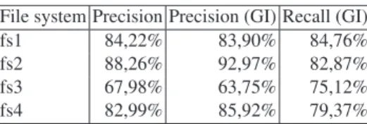
The results are summarized in Table 2. In the second column of the table, a global measurement representing the precision ofgreat increase(GI) andother changes(OC) labels together is shown. The precision and recall values for the GI label are shown in the third and fourth columns.

File system Precision Precision (GI) Recall (GI) fs1 84,22% 83,90% 84,76% fs2 88,26% 92,97% 82,87% fs3 67,98% 63,75% 75,12% fs4 82,99% 85,92% 79,37%

Table 2.Summarized cross-fold validation test results of MORI for predicting file system changes

The prediction was the worst in the case offs3, which could be caused by the fact that this file system had the largest bound (see Table 2). However, we cannot state that the results have a strong correlation with the automatically determined bounds because the best result is produced in the case offs2, which has the second largest bound. To

sum up, the results are promising, but we have to make further examinations.GIlabels are much frequent in certain time intervals than in the other cases. In these intervals, the machine learning model reached very good local results, but in the other cases, it was not so precise. For example, in the case offs2, there were three partitions on the whole timeframe where theGIlabels were almost constantly experienced. For these cases, the machine learning algorithm worked very well, but in the other cases when theGIlabels were experienced infrequently, it could not give the same good results.

3.2 Prediction of problematic events

We applied theCAmethod (see Section 2.3) to predict whether a problem event would occur in a certain time or not. CA was run on the previously collected data of the sub-ject system (from June 6, 2007 to January 17, 2008). During this interval, the customers reported five problems with the subject system (August 21, 2007; September 25, 2007; October 12, 2007; October 26, 2007; January 9, 2008). We applied CA for these prob-lems, and used five-cross-fold validation for testing the machine learning models.

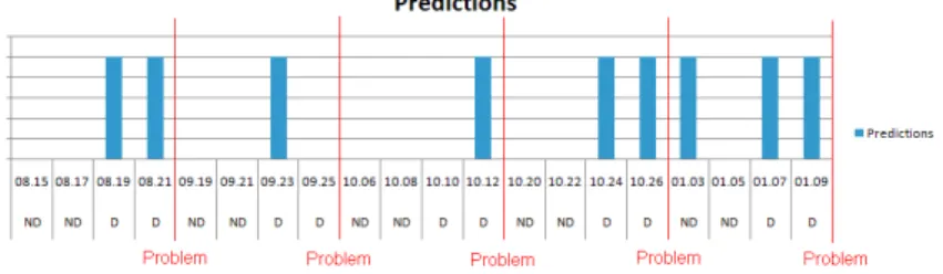
After several experiments, we managed to select the appropriate arguments for CA: the size of the preceding interval (PI) was 8 days with two ND and two D labels. This way, an ND and a D label represented a two day long subinterval. In the next step, we tried out several machine learning algorithms, and finally the Logistic Model Tree (LMT) [9] was the best. Table 3 shows the statistics based on the 5-cross-validation results, while Figure 4 shows the concrete predictions. On the X axis, the ND and D labels are shown for the five problems, while on the Y axis the prediction results of the machine learning algorithm are shown: if the machine learning algorithm predicts D, the value is represented with a column. Above the ND and D labels, the endpoint of the two day long interval is shown. For example, in the case of the first column, it means that the interval lasted from midnight 13th August to midnight 15th August. Based on Figure 4, it can be said that the machine learning algorithm can forecast every problem, but in certain cases, it makes forecast even if it is not needed (01.03).

Precision Precision (D) Recall (D) 85% 88,9% 80%

Table 3.Summarized cross-fold validation test results of CA for predicting problems

We investigated the machine learning models and realized that very good predictor pairs came from the predictor groups of:

– disk usage-disk usage: it means, that certain disk drives’ correlation changes when a problem arising.

– theapplication error and log dataand thedisk usage, which imply that the connec-tion of certain applicaconnec-tion events with certain disk usage changes when a problem arising.

– whether the root logged inand thedisk usage. This is really surprising, but can be happened. The simplest explanation is the following. If an administrator is logged in, then she can listen to the disk usage and can precede the fullness of a disk. It is also explain, why our industrial partner drawn our attention to the fullness of the disk drives.

The success of this method depends on the applied parameters, which are currently based on our experiments. Determining these parameters effectively is yet another prob-lem, which could be solved by introducing a new machine learning phase in CA in the future. However, it is questionable whether the machine learning algorithm model forecasts problems for intervals when the problems are far away. To examine this ques-tion, we selected the following dates: 11.18, 11.26, 12.10 and 12.18. CA was run for these dates similarly as before (preceding 8 days with two ND and two D labels). This means 16 predictions. In these cases, the previously produced machine learning algo-rithm model did not forecast any problems correctly.

Fig. 4.Predictions of problems with CA method

We experienced that the correlation anomalies method could be a good solution to forecast the problems. To sum up, for a complete validation of this technique, we have to make further investigations and try out other test cases.

4 Related work

In this Section we present an overview of the research area of predicting runtime prob-lems in software systems.

Chen et al. [10] presented a similar work. They used the abnormal change of distri-bution of certain extracted statistics about the system which is similar to our CA data transformation method. They presented their new approach to detecting and localizing service failures in component based systems. They tracked high dimensional data about component interactions to detect failure dynamically and online. They divided the ob-served data into two subspaces: signal and noise subspaces, and extracted two statistics that reflected the data distribution in subspaces for tracking. The subspaces are updated for every new observation, data distribution is learned. This decomposition method is

not a novel approach but they employed online distribution learning algorithms instead of normal distribution.

Wolski presented [11] a similar method to MORI. The author focused on the dy-namic prediction of network performance with the support of parallel application scheduling. A prototype of Network Weather Service (NWS) was developed to forecast future latency, bandwidth and available CPU percentage for each monitored machine. Three kinds of forecasting methods were implemented: mean-based, median-based and autoregressive method. NWS automatically identifies the best prediction method for the resource.

Cohen et al. [12] were applied Tree-Augmented Bayesian Networks (TANs) to find correlation between certain combinations of system-level metrics and threshold values and high-level performance states in a three-tier web service. This paper showed that TANs are powerful enough to recognize the performance behavior of a representative three-tier web service. It can forecast violations with stable workloads as well.

A new concept named flow intensity was introduced by Jiang et al. [13] to measure the intensity with which the internal monitoring data reacts to the volume of user re-quests in distributed transaction systems. They gave a new approach to automatically model and search relationships between the flow intensities which are measured at var-ious points of the system.

Munawar et al. [14] presented a new approach to monitoring at a minimal level in order to determine system health and automatically adaptively increase the monitoring level if a problem is suspected. The relationships between the monitored data were used to determine normal operation and – in the event of anomalies – identify areas that need more monitoring. In this paper the authors urged the need for adaptive monitoring and describe an approach to drive this adaptation.

Kiciman et al. [15] presented Pinpoint, a methodology for automating fault detec-tion in Internet services by observing the low-level, internal structural behaviors of the service. It modeled the majority behavior of the system correctly and detects the anoma-lies in these behaviors as the possible symptoms of the failures.

Ostrand et al. [16] assigned a statistical model with a predicted fault count to each file of a new software release based on the structure of the file and its fault and change history in previous releases. The higher the predicted fault counts, the more important it is to test the file early and carefully.

5 Conclusion

During this work, we tried out different data filtering techniques, data transformation methods, and several machine learning algorithms. When forecasting the changes of the file systems and the problems, we achieved promising results, which give bases for further work. However, there are several opportunities to continue this work. First, the presented methods could be tried out on further data and should be integrated into the subject system to get an online forecasting system. To improve the precision of the predictions, the development of other data transformation methods is possible. For ex-ample, in the case of the MORI method, it would be useful to investigate the relationship between the changes of the file system and the reported problems. Furthermore, another

important task is to set the parameters of the data transformation methods automatically, which can be supported by machine learning algorithms as well.

Acknowledgements. This research was supported in part by the Hungarian national grants RET-07/2005, OTKA K-73688, TECH 08-A2/2-2008-0089 (SZOMIN08) and by the J´anos Bolyai Research Scholarship of the Hungarian Academy of Sciences.

References

1. Luckham, D.C.: The Power of Events: An Introduction to Complex Event Processing in Distributed Enterprise Systems. Addison-Wesley Longman Publishing Co., Inc., Boston, MA, USA (2001)

2. Witten, I.H., Frank, E.: Data Mining: Practical machine learning tools and techniques. Mor-gan Kaufmann, San Francisco (2005)

3. Alpaydin, E.: Introduction to Machine Learning. MIT Press (2004)

4. Picard, R.R., Cook, R.D.: Cross-validation of regression models. Journal of the American Statistical Association79(1984) 575–583

5. Breiman, L., Friedman, J., Olshen, R., Stone, C.: Classification and Regression Trees. Wadsworth and Brooks, Monterey, CA (1984)

6. Wasserman, P.D.: Neural computing: theory and practice. Van Nostrand Reinhold Co. New York, NY, USA (1989)

7. Mitchell, M.: An Introduction to Genetic Algorithms. MIT Press (1998) 8. Quinlan, J.: C4.5: Programs for Machine Learning. Morgan Kaufmann (1993)

9. Niels Landwehr, M.H., Frank, E.: Logistic model trees. In: Springer ’05: Machine Learning, Springer Netherlands (2005) 161–205

10. Chen, H., Jiang, G., Ungureanu, C., Yoshihira, K.: Failure detection and localization in component based systems by online tracking. In: KDD ’05: Proceedings of the eleventh ACM SIGKDD international conference on Knowledge discovery in data mining, New York, NY, USA, ACM (2005) 750–755

11. Wolski, R.: Forecasting network performance to support dynamic scheduling using the net-work weather service. In: Proceedings of the 6th IEEE International Symposium on High Performance Distributed Computing. (1997) 316–325

12. Cohen, I., Goldszmidt, M., Kelly, T., Symons, J., Chase, J.S.: Correlating instrumentation data to system states: a building block for automated diagnosis and control. In: OSDI’04: Proceedings of the 6th conference on Symposium on Operating Systems Design & Imple-mentation, Berkeley, CA, USA, USENIX Association (2004) 231–244

13. Jiang, G., Chen, H., Yoshihira, K.: Modeling and tracking of transaction flow dynamics for fault detection in complex systems. IEEE Transactions on Dependable and Secure Comput-ing3(2006) 312–326

14. Munawar, M.A., Ward, P.A.S.: Adaptive monitoring in enterprise software systems. (In: In SysML, June 2006.)

15. Kiciman, E., Fox, A.: Detecting application-level failures in component-based internet ser-vices. Neural Networks, IEEE Transactions on Neural Networks16(2005) 1027–1041 16. Ostrand, T.J., Weyuker, E.J., Bell, R.M.: Predicting the location and number of faults in large