Neural modelling of ranking data with an application to stated preference data

NEURAL MODELLING OF RANKING DATA WITH AN APPLICATION TO STATED PREFERENCE DATA

C. Krier, M. Mouchart, A. Oulhaj1

1. INTRODUCTION

Many business and social studies require modeling individual differences in choice behavior by asking respondents to rank alternatives. However, this kind of data present some particularities, related to their non-continuous and bounded character that should be taken into account by the models.

Neural Networks (NN) provide an approach that progressively attract more at-tention from statisticians working in a wide variety of problems. Some examples issued in Statistica give an interesting view of the variety of topics faced with a NN approach. Thus, Apolloni et al. (2001) considers a forecasting problem con-cerning quality characteristics of bovine; Biganzoli et al. (2000) proposes the automatic learning process of a NN for the study of complex phenomenon in biostatistic; also Pillati (2001) proposes to combine radial basis function networks and binary classification trees. The object of this work is to model with NN the firm’s preferences, in particular the relative importance of each attribute, in the firm’s ranking procedure.

The data used to illustrate the method consist of rankings of alternative solu-tions for freight transport provided by different companies through face-to-face interviews. These transport scenarios are defined by six attributes: frequency of service, transport time, reliability, carrier’s flexibility, transport losses, and cost. Further details are given in section data and a more systematic presentation of the data may be found in Beuthe et al. (2005).

The paper presents first the data used to illustrate the method. Section 3 scribes the assumptions made in connection with the firm’s decision rule, and de-tails the form considered for the underlying utility function. The estimation of the

firm’s decision rule is developed in Section 4, which is organized as follows: a general view of the perceptron structure is presented, followed by a short descrip-tion of some traps which should be avoided. The last part of this secdescrip-tion relates to the heuristic chosen to perform the minimization implied by the perceptron algorithm. Section 5 provides information on how the experiments were carried out, shows some results on the data and discusses them.

2. NEURAL NETWORKS APPROACH FOR RANKING DATA

Ranking data are obtained when I objects zi J(i1... )I are ranked from 1 to I. A basic difference between “ordinal data” (i.e. data measured on an ordi-nal scale) and “ranking data” is that ordiordi-nal data are measured on a scale with far less degrees than the sample size; in contrast, the scale for ranking data has as many degrees as the sample size.

Thus ties – or ex aequo – are dominating in ordinal data, but scarce, and some-times excluded, in ranking data.

Figure 1 – Neuron n of layer (l ).

Beuthe et al. (2008) compares the analysis of ranking data under models adapted from models originally developed for ordinal data (such as ordered logit, conjoint analysis or UTA type models). In theoretical statistics, the distribution of rank statistics has been developed for the case of observable variables. This paper develops a model based on the idea of interpreting ranking data as rank statistics of a latent variable, namely the value of a latent utility function defined on the characteristics of the ranked objects.

The modeling strategy is based on a neural approach. For the sake of more specificity, suppose that we observe the ranking of I objects identified by J characteristics. The data consist therefore of an (I J ) – matrix

1 2 [ ] [ , , ..., ]ij I

Z z  z z z  where zi J represents the J characteristics of the

1 2 ( , ,..., I)

R R R R , where Ri denotes the rank of the i th object. To each ob-ject i we associate a latent utility ui and therefore obtain an I-dimensional latent vector u( , ,..., )u u1 2 uI .

Generally speaking, a multi-layer perceptron consists of several layers of weights and neurons which present the configuration illustrated in Figure 1. The output ( 1)l

n

x  of one neuron can be used as an input for one or several neurons belonging to the next layer. Non-linear activation functions ( )l

n

 are associated to each neuron. This makes the NN framework suitable for developing learning al-gorithms as a possible approach to iterative procedures used for complex statisti-cal inferences as exemplified in Section 4. Let us statisti-call ( )l

nd

w the weights associated to the neuron n and input d of the layer l, the output of the layer l is

( ) ( ) ( ) ( 1)

1

. D

l l l l

n n nd d

d

x  w x 



 

 _{ }





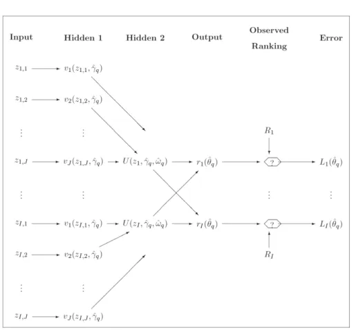
From a neural perspective, we may therefore view the u- and v-vectors (see equations (5) and (6)) as hidden layers of a multi-layer perceptron (more details in Bishop (1995) and Haykin (1999)), the structure of which is detailed in Figure 2. Finally, the target function aggregates the squared differences between the ob-served ranks Ri and the rank statistics of the estimated latent utilities.

3. STATISTICAL MODELLING

3.1 The firm’s decision rule

The decision maker (d.m.) is assumed to make his choice as follows:

( )i To each scenario zi he associates a utility U z( , )i i depending on the rele-vant and known characteristics, or attributes, (zi) and on characteristics of events which are uncontrolled and unknown and that also affect the decision maker’s utility (i).

( )ii The utilities U z( , )_i _i are random for the decision maker because they de-pend on the unobservable vector ( , ,..., ) 1 2 I . Under an expected utility as-sumption, the d.m. computes for each scenario zi the expectation of these ran-dom utilities, namely:

( , )i [ | , ]i

U z  _U z  ₍₂₎

( )iii The observed ranking Ri is interpreted as an ordering, over the I scenarios, of the expected utilities U z( , )i  , 1 i I. Therefore, the theoretical rank

( , ) i

r Z  is given by:

{ ( , ) ( , )} 1

( , ) 1 _i

i I

i U z U z

i

r Z   

 



 



where 1_{.} represents the indicator function. Thus ( , ) 1r Zi   is given to the scenario with lowest utility.

Because the rank statistic ( , )r Z  is not sufficient for the utility vector u, the transformation (3) leads to an identification problem (see Oulhaj and Mouchart, 2003). More specifically, for a given set Z of scenarios, the ranking function

( , )

r Z  defined by

1

( , ) : ( , ) ( ( , ),..., ( , ))I

r Z  Z   r Z  r Z  (4)

is not one-to-one. This means that different values of  may correspond to a same ranking.

3.2 A parametric utility

The following parametric specification for U is considered:

1

( , ) ( , ) 1

J

i j j ij

j

U z   v z  j I







where , 1vj  j J, are known functions and ( , ) is the parameter of in-terest. The parameter ( , 1 2,...,J) lies in the (J1) dimensional simplex

1 [J 1] { J| Jj j 1}

S   s  s  , and  are parameters of vj.

We pay a particular attention to a logistic specification of the utility function, namely:

( )

1

( , , )

1 1

j j ij

j j ij j j ij z

j ij j j z z

e v z e e              

  (6)

1 1

, 1 1,

1 j p j _J p e j J e    _     

  (7)

1 1 1 1 p J _J p e   _  

  (8)

where 1

1 2 1

( , ,..., ) J

J

    

 

  . The inverse transformation is

1

, 1 1.

1 j j

p j p

ln  j J

       _ _     

  (9)

This relation characterizes a bijection between the interior of S_[J_1] and J1.

The parameter vector to be estimated,  ( , )  , has accordingly dimension 3J1.

4. NEURAL ESTIMATION

The objective of this section is to build an estimator of  minimizing a loss function ( )L  which aggregates a loss Li( ) associated to each scenario

1,...,

i I, viz.

1 ( ) I _i( ).

i

L  L 







Under a neural approach, the iterative algorithm generates a sequence of esti-mates ˆ_q(q0) following the structure illustrated in Figure 2. This algorithm, re-peated independently for each firm, presents the structure of a perceptron with two hidden layers and proceeds as follows:

0. Input the I scenarios Z[ ]z_i , the observed ranks R( ,...,R1 RI) and an ini-tial value ˆ0.

1. Compute U z( , )_i ˆ_q 1 i I (from (5) and (6)).

2. From equation (3), compute the estimated ranking r Zi( , )ˆq .

3. Knowing r Zi( , )ˆq and the observed rank of zi (i.e. Ri) for each scenario, evaluate the loss associated to the ranking error of the scenario i, namely:Li( )ˆq . Then compute the total loss function L( )ˆq (from (10)). 4. Update the parameter ˆ_q. The update is based on the minimization of the

to-tal loss function L( )ˆ .

Figure 2 – Perceptron structure (for  ˆ ˆq( ˆq q,ˆ ) at the q-th iteration).

The error criterion to be minimized takes into account the discrete character of the observed ranking, and the continuous character of the hidden (latent) utility function (5) and (6). A natural solution is to use the quadratic error between the stated ranking R_i and the estimated ranking ( , )r Z_i  produced by the model namely:

2

1

( ) I ( ( , ) ) .

D i i

i

L L  r Z  R



 



Remark:When fitting ordinal data, minimizing the quadratic error (11) might seem less attractive than maximizing the Kendall coefficient, namely

1 2 ˆ

( , ) ,

( 1)

K

S R R

I I

 

 (12)

ˆ ˆ {( )( ) 0}

1 1,

2 1

. i j i j

ij R R R R

ij i I j i

S S S           



Both criteria correspond to closely related ideas and may be expected to pro-duce similar results. In particular, in the case of perfect fit (i.e. Ri Rˆ ,i i),

ˆ

( ) 0 D

L   and  _K( ) 1ˆ  . In the application, we systematically optimize L_D for being numerically more stable than _K.

5. APPLICATION

5.1 The data

For a given firm, we observe I 25 scenarios and a corresponding ranking. Each scenario is represented by a vector of J 6 attributes. By convention, z1 stands for a reference scenario. We denote by Z the (25 6) matrix containing all the 25 scenarios. The ranking of these scenarios is represented by a vector

1 2 25

( , ,..., )

R R R R where Ri denotes the rank of zi according to the firm’s preference. The ranking Ri of each scenario lies eventually between 1 and 25 . Thus, for each firm we have a (25 7) data matrix ( , )Z R . The rankings of 9 firms have been treated independently of each others.

5.2 Pitfalls in minimization

Equation (3) makes clear that ( , )r zi  and therefore LD( ) (where D stands for discrete), are not continuously differentiable in . Its minimization cannot be carried out by classical algorithms such as gradient methods. In order to circum-vent this difficulty, one might think that the rankings behave as a discrete ap-proximation of a utility scaled to lay in [1, 25] . This may be achieved through the following transformation of ( , )U zi  :

( , ) ( )

( , ) 1 24 [1, 25]

( ) ( )

s i

i

U z m

U z M m        

  (13)

where m( ) min U zi ( , )i  and M( ) max U zi ( , )i  . Thus, ( )m  (resp. M( ) ) is the lowest (resp. highest) utility. In this case, the loss function can be written as follows:

25

2

1

( ) ( s( , ) )

C i

i

L L  U Z R



where C stands for continuous. The loss function LC( ) is differentiable and can be minimized by a gradient method.

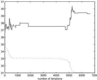
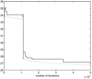
Experience has however revealed that such an approach raises substantial problems. For two selected companies, we observed the following difficulties. In Figures 3 and 4, we plot, for 2 different firms, in plain line the value of LC( )ˆq and in dashed line, the corresponding value of L_D( )ˆ_q , as functions of the num-ber of iterations. Figure 3 shows that minimizing LC may be conflicting with minimizing L_D. Figure 4 reveals that, for another company, assessing whether the algorithm has achieved a reasonable neighborhood of the true minimum may be problematic because the decrease of the objective function may have an un-usual behavior: will the steep decrease around the 1000-th iteration repeated later on? after the iteration 100 000? and is the value of the objective function, namely 26, far or close to the true minimum? The maximum ranking error LD among J alternatives, say ( )M J , is equal to

| /2|

2

( ) 2 ( 2 1)

J

M J 



where | |a stands for the integer part of a. Thus, with 25 alternatives, we know that 0  LD  5200.

Figure 3 – Evolution of the discrete loss function LD (plain line) and the continuous loss function

C

L (dashed line) in function of the number of iterations for company 4.

0 1000 2000 3000 4000 5000 6000 7000

31 32 33 34 35 36 37 38 39 40 41

5.3 A heuristic Approach

The unsatisfactory results and the problems related to the approximation of the discrete loss function LD by the continuous loss function LC lead us to look for an alternative approach. Minimizing the discrete error LD fosters the use of non classical techniques able to deal with a discontinuous criterion.

In the present case, the heuristic allowing the minimization is based on the Pocket algorithm Gallant (1996). Similarly to a gradient method, the Pocket algo-rithm generates a sequence of estimates ˆq. One major difference is that the computation of ˆq1, as a transformation of ˆq, is obtained through an iterative procedure with steps indexed by, say, t . In this application, there are 17 parame-ters (see equations (6) to (9)), but, as each step t may require a positive or a nega-tive variation, the Pocket algorithm considers 34 possible variations to be evalu-ated. Thus the 17-dimensional vector  (_f ) is replaced, in the Pocket algo-rithm, by a 34-dimensional vector (_{f s,} ) with f 1,...,17 and s  1, 1.

Figure 4 – Evolution of the discrete loss function L_D (plain line) and the continuous loss function

C

L (dashed line) in function of the number of iterations for company 9.

Two types of parameters characterize a Pocket algorithm, namely a fixed num-ber (D) of coordinates ( , )f s to be updated at each step t and a length of adap-tation (_f ), kept constant at each step t. For simplicity, let us consider a par-ticular iteration q and write ˆ instead of ˆq, where ˆ has coordinates ˆf s, The sequence ˆ_{f s,} ( )t is generated as:

0 1 2 3 4 5

x 104

26 27 28 29 30 31 32 33 34 35 36

, , {( , ) }

ˆ _{( 1)} ˆ _{( ) ,}

t

f s t f s t f s A s f

   1   (16)

where At selects, among all possible ( , )f s , the D most favorable ones, i.e. the updates corresponding to the steepest decrease of squared error LD eliminating those coordinates for which sf increases LD. Thus the step t is final once

1 t

A becomes empty. Obviously D2F, where F stands for the number of

parameters to be optimized; here F 3J 1 17.

5.4 Choice of the parameters for the iterative procedures

For the initialization of the perceptron procedure, the weights j are set equal to values declared in the interviews when available, this is the case for companies 2, 3, 4, 6, 7, 8 and 9. For the other companies, namely companies 1 and 5, the initial weights are set equal to those obtained in a UTA model developed in Beuthe et al.

(2008). The other parameters,  and  , are initialized to 1. The number of itera-tions is fixed at 200; the same number of iteraitera-tions is used for all simulaitera-tions.

A simple run of the Pocket algorithm described above is quick but the reliability of the results crucially depends on the specification of F1 parameters required by the working of the algorithm, namely D and f with f 1,...,F. It is there-fore compelling to input several trial values for these parameters. In the present application, the optimization for each firm is organized as follows:

 D varies between 1 and 17 by steps of 1

 the length of adaptation for the  and  parameters varies from 0.1 to 1 by steps of 0.1

 the length of adaptation for  varies from 0.0005 to 0.002 by steps of 0.00025.

The variation for the length of adaptation of  is chosen lower than that of 

and  because of the high impact of a variation of  in the value of . As a matter of fact, the problem is quite sensitive when the number of updates per step (D) is high. The best model can be selected according to the loss function

D

L or the K. Because the evaluation of K is not computationally convenient, we systematically minimize LD and report the results and the K for the models reaching the smallest value of LD and the highest value of K respectively; when the two models coincide, we write LD~K.

5.5 Results for freight transport data

Let us first examine Table 1. For Companies 1, 2, 4 and 5, the models with lowest L_D and highest _K are different but the corresponding _K ’s are close to-gether (for instance, .9067 and .9133 for company 1, .8867 and .9000 for com-pany 2) and the estimates of the weights are also similar. For the other compa-nies, namely companies 3, 6, 7, 8 and 9, the two models are the same. The fact that all methods, estimated in Beuthe et al. (2006), lead to models whose K is one for company 9 suggests that the behavior of this firm is quite simple and that all models overfit. It is likely that this phenomenon of overfitting occurs in several cases. Indeed, it is questionable that a model could approximate the be-havior of a company in terms of choice of transportation mode in such way that the Kendall coefficient would reach 0.9000. The fact that the NN method counts less parameters than UTA and leads to lower K is reassuring from this point of view.

TABLE 1

Weights for each model and Kendall coefficient

Table 2 shows that the estimation of the  ’s is reasonably robust with respect to the choice between the two criteria LD or k: they keep the same sign and the same order of magnitude, with however one noticeable exception for company 2 where the estimations differ substantially, in sign and in order of magnitude, for Reliability and Flexibility. This may be taken as a signal numerical sensitivity due to the discreteness of the rankings.

corresponding values of the  parameters support this observation. On the con-trary, the Loss attribute seems unimportant with respect to the values of the weights, which are less or equal to 7% , except for company 2. Reliability has also an impact for some companies. Company 4 presents an atypical behavior: its main attribute is Frequency, followed by Time.

TABLE 2

Values taken by  parameters for each company

The sign of the  parameters expresses the favorable (when positive) or unfa-vorable impact (when negative) of the related attribute. Attributes whose weights in the model are close to zero are not significant and should not be taken into ac-count when interpreting the corresponding values of  and .

We may notice in general that the results for both criteria of selection (loss function and Kendall) lead to the same model or to models rather similar in terms of performances and relative importance of the attributes. The other parameters seem however less stable.

TABLE 3

Values taken by  parameters for each company

6. CONCLUSION

This paper shows that a perceptron model can lead to a good prediction of the ranking. In addition, the parameters of the model express correctly the negative or positive impact of an increase in an attribute level, in most cases. The weights of the model give an insight about the relative importance of each freight trans-port attribute. In particular, it is shown that Cost and Reliability are often the most important features.

A continuous approximation of the quadratic error between the ranking and its estimate is not always suitable. Indeed, the minimization of the quadratic error and the continuous approximation may be conflicting. Also, the behavior of the continuous approximation make the minimization by a gradient method difficult.

ver-sion of UTA with less parameters. The description and comparison of these models can be found in Beuthe et al. (2008). However, those methods do not provide results easily interpretable, contrarily to the perceptron model.

OS Engineer, KPN Group Belgium CATHERINE KRIER

CORE and ISBA, Université catholique de Louvain MICHEL MOUCHART

DTU, Nuffield Department of Clinical Medecine ABDERRAHIM OULHAJ

University of Oxford

REFERENCES

B. APOLLONI, I. ZOPPIS, R. ALEANDRI, A. GALLI,(2001), A neural network based procedure for

forecast-ing bovine semen motility, “Statistica”, LXI (2), 301-313.

M. BEUTHE, CH. BOUFFIOUX, J. DE MAEYER, G. SANTAMARIA, M. VANDRESSE, E. VANDAELE, F. WITLOX, (2005), A multi-criteria methodology for stated preferences among freight transport alternatives, in AURA REGGIANI and LAURIE SCHINTLER (ed.) Methods and Models in Transport and

Communica-tions: Cross Atlantic Perspectives, Berlin: Springer Verlag.

M. BEUTHE M., CH. BOUFFIOUX, C. KRIER, M. MOUCHART, (2008), A comparison of conjoint,

multi-criteria, conditional logit and neural network analyses for rank-ordered preference data, chap. 9 in M.

BEN-AKIVA, H. MEERSMAN and E. VAN DE VOORDE (ed.) Recent Developments in Freight

Trans-port Modelling: Lessons from the Freight Sector, Emerald Group Publishing Limited,

157-178.

M. BEUTHE, G. SCANNELLA,(2001), Comparative analysis of UTA multi-criteria methods, ‘European Journal of operational research’, 130 (2): 246-262.

E. BIGANZOLI, P. BORACCHI, I. POLI, (2000), Reti neurali artificiali per lo studio di fenomeni complessi:

limiti e vantaggi delle applicazioni in biostatistica, ‘Statistica’, LX (4), 723-734

C.M. BISHOP, (1995), Neural Networks for Pattern Recognition, Oxford: Oxford University Press.

S.I. GALLANT, (1996), Perceptron based learning algorithms, ‘IEEE Transactions on Neural Net-works’, 1:179-191.

S. HAYKIN, (1999), Neural Networks: a comprehensive foundation, 2nd ed., Prentice-Hall, Inc. A. OULHAJ, M. MOUCHART, (2003), Partial sufficiency with connection to the identification problem,

‘Metron’, LXI (2), 267-683.

M. PILLATI, (2001), Le reti neurali in problemi di classificazione: una soluzione basata sui metodi di

segmentazione binaria, ‘Statistica’, LXI(3), 407-421

H.R. VARIAN, (1992), Microeconomic Analysis, 3rd ed., Norton & Company, New-York.

SUMMARY

Neural modelling of ranking data with an application to stated preference data