Vol.3 No.4, 2019
Abstract— With the adaptation of traditional image processing methods to answer to the requirements of analyzing more complex representations than the standard gray scale portrayal, a growing interest is directed towards color image processing. Many color spaces are suggested in the literature, each serving a defined purpose and generating an output image with distinguishable perceptual differences. One other major difference between existing color spaces is the meaning each of them gives to the color component that makes certain operations and transformations possible on a representation and not on another. This raises the question whether certain processing may score distinct results on different color spaces. In this paper, we investigate the impact of RGB and HSV color representations on one of the well-known segmentation methods: the Seeded Region Growing algorithm (SRG). The adopted segmentation approach consists of three major steps: 1) The automated seed selection, based on two criteria, 2) The region growing phase, that will gather neighboring pixels and seeds into regions according to a similarity rule guided by the Euclidean distance, and at last, 3) the region merging phase will proceed to overcome the over segmentation issue and enhance the meaning of the defined regions will improving the segmentation accuracy. Three metrics from the literature were used to assess the performances of our algorithm on both color spaces conforming to similarity, distortion and noise. The segmentation results were compared by combining and averaging the performance measures from an images sample from the Berkeley dataset. The algorithm showcased more accurate results and consumed less execution time in the HSV color space compared to the RGB one. Post processing steps were tested and included in the RGB model to enhance the segmentation outcome.
Manuscript submitted December 31, 2018. This work was supported in part by the R&D department of OCP group, the OCP foundation, the Mohammed VI Polytechnic University, the National Center of Scientific and technical Research (CNRST), and the Ministry of Higher Education, Scientific Research and Professional Training of Morocco (MESRSFC).
R. C. Author is with the Faculty of Science and Technology, LERSI, University Sidi Mohammed Ben Abdellah, Fes, Morocco, and with the Embedded System Department, Mascir, Rabat, Morocco (e-mail: rajaa.charifi@usmba.ac.ma).
N. E. Author is with the Faculty of Science and Technology, LERSI, University Sidi Mohammed Ben Abdellah, Fes, Morocco (e-mail: [email protected]).
A. M. Author is with the National School of Applied Sciences (ENSA), University Sidi Mohammed Ben Abdellah, Fes, Morocco (e-mail: [email protected]).
Y. Z. Author is with the Embedded System Department, Mascir, Rabat, Morocco (e-mail: [email protected]).
Index Terms— Color image Segmentation, region growing, seed selection, region merging, Structural Similarity Index, Mean Square Error, Peak Signal to Noise Ratio, Median filter.
I. INTRODUCTION
N remote sensing, segmentation occupies and ensure a major role, prior to the high-level processing in which recognition and identification of the object of interest are made. This mid-level processing step enables the distinction between elements of predefined “inhomogeneity” degree and the grouping of pixels sets into super-pixel regions, based on the study of local features including, among others, color and texture features. During the past decades, many approaches have been elaborated, each showing strengths and weaknesses depending on the studied case. Based and the principle and techniques used, segmentation algorithms can be grouped into five major categories [1]:
Threshold based techniques: As the most basic type of segmentation algorithm and the simplest, the thresholding based segmentation algorithms make use of the histogram information to decide about the partitioning of a given image. In this category alone, many types of thresholding methods can be found, each using a certain type of information and delivering variant results depending on the studied images type [2].
Edge based techniques: As its name indicates, the algorithms of this category proceed by depicting the strong edges followed by filling the defined areas to obtain a segmentation result. One major drawback of these techniques is the sensitivity towards the noise. However, when adapted and well-tuned, the results can be very promising, especially with watershed and snake-based algorithms [3] [4]
Region based techniques: Unlike the edge based methods, region-based techniques follow a reversed approach under which the fill of a region is defined, beginning from a starting point called seed, then the contours are drawn around the found regions.
Clustering techniques: The aim of these techniques is to assemble found patterns from a previous segmentation stage into groups using distance calculations [1].
Matching techniques: These supervised techniques require disposing of ground truth references to which the segmentation results will try to match.
Studying the Impact of the Color Representation
Choice on Segmentation Results by the Seeded
Region Growing Algorithm
Rajaa Charifi, Najia Es-sbai, Anass Mansouri,
Member, IEEE,
and Yahya Zennayi
Vol.3 No.4, 2019 The previously mentioned classes are not strictly distinct and
disassociated but share some common properties. This intersection aspect encourages the birth of a multitude of hybrid approaches capable, in a complementary way, of delivery even better results [5]. One famous output of the segmentation algorithms hybridization is the Seeded Region Growing algorithm [6]. As a region-based segmentation technique, the SRG requires the identification of start pixels, also named seeds, from which the growing process is going to follow up. The emphasis of this step on the segmentation led many studies towards investigating different seed choice criteria [7] [8] [9], guiding the growing process afterward. From each start pixel, defined as the region’s core, the growing process includes neighboring pixels under a regularized similarity assessment. Many reasons lie behind the success scored by the SRG segmentation method. In addition to the possibility of tuning and supervising the seed selection stage, it delivers rapid and accurate results and doesn’t require ground truth or training sets. However, implementing SRG algorithm alone tends to produce over-segmented results and inserting some guiding criteria along the algorithm or adding other processing steps proves to be useful for enhancing the quality of the segmentation outcome [10] [11].
Adapting the SRG segmentation method to high dimensional images is very straightforward. As a result, SRG was the subject of many studies working on color images. Fan & al. choose implementing the concerned segmentation algorithm on the YUV (Luma and two chrominance) color representation [12]. It was found that using isotropic color edge detectors to define the seeds of the growing algorithm makes the technique adequate for advanced application such as human face recognition. Later on, Frank Y. Shih and Shouxian Cheng approached the same color space with different seed selection and post-processing techniques [13]. HSV (Hue Saturation, Value) space segmentation was investigated by Huang & al. and delivered visual satisfying results compared to Frank Y. Shih and Shouxian Cheng study [14] [13]. Concerning the conventional RGB (Red, Green, and Blue) color space, Guthal & al. worked on each color channel separately as an independent image on which the SRG algorithm was run [15].To underline the major differences and intersections between the previous studies, a concise description of the used methods is presented in Table.Ⅰ.
Our achieved work fits in the context of studying and assessing, in a quantitative way, the relationship between the rightness and the precision of the segmentation results and between the color representations chosen to display a given database. Two color representations will make the fundaments of our study: the HSV and the RGB spaces. A comparison between the two representations-SRG-segmentation-outputs will be made upon the accuracy, the precision and the response time using some of the most reliable metrics in the literature. The remainder of this work is organized as follows. In section II, we present and explain our used algorithm while underlining its shades between the two color spaces. Section III is a brief overview of the metrics used. In IV, we introduce
the study context of our work to pave for the next section, V, in which the results of the algorithm are demonstrated. The main conclusions are reiterated in the last section VI.
II. METHODS AND PROPOSED APPROACH
For clarification reasons, the projection of a studied image on the RGB and HSV color spaces will be referred to, respectively, as 𝐼𝑟𝑔𝑏 𝐼ℎ𝑠𝑣.Each pixel will have, in addition to its spatial coordinates (i,j), three color components: 𝐼𝑟𝑔𝑏(𝑖, 𝑗) = (𝑟(𝑖, 𝑗); 𝑔(𝑖, 𝑗); 𝑏(𝑖, 𝑗)), 𝐼ℎ𝑠𝑣(𝑖, 𝑗) = (ℎ(𝑖, 𝑗); 𝑠(𝑖, 𝑗); 𝑣(𝑖, 𝑗)). The spatial size of each image is equal to M*N, where M and N are the number of rows and columns, respectively.
A. Automatic Seeds Selection Process
Defining the seed or seeds from which the growing process will initial is the most crucial phase of our segmentation process. As seen in Table.Ⅰ, many criteria can be used as selection criteria, either alone or combined. In our work, we choose to use two norms: The no-edgness and the color-similarity verified for each pixel I(i,j) on a neighborhood defined by a 3*3 window[14][16].
• No-edge Criterion: A pixel is considered edge belonging when its intensity level marks an abrupt change from a pixel to another connected pixel. To evaluate this, we compute the G image of the HSV colored image, where each pixel g(i,j) is represented by the average of the hue over I(i,j) pixels’ 3*3 neighborhood. The G image is defined as follows:
𝐺 = {𝑔(𝑖, 𝑗); 0 ≤ 𝑖 ≤ 𝑀, 0 ≤ 𝐽 ≤ 𝑁 𝑔(𝑖, 𝑗) =1
9∑ ∑ ℎ(𝑘, 𝑙) 𝑗 𝑙 𝑖 𝑘
(1)
The next step involves computing the average 𝑎𝐺and the standard deviation 𝜎𝐺 over the G image. This two parameters will be used to set the used threshold for seed pixels selection as expressed in (2), and each pixel with a g value under the threshold will be labeled as a seed and added to the seeds list.
TABLEI
SRGAPPLIED METHODS ON DIFFERENT COLOR SPACES
Color Space Data set Seeds selection criteria
Post processing to the SRG algorithm
Fan &
al. [12] YUV
Rando m set Isotropic Color edge detectors
Spanning Tree for insignificant edges removal
Frank Y. Shih and Shouxian Cheng
[13]
YUV Rando m set
Color composit
e deviation
Region merging based on color then size thresholding
Huang & al. [14] HSV
Rando m set
Edge and smoothne ss criteria
Region merging based on color and on size
thresholding
Guthal & al.[15]
RGB Berkele y
Intensity similarity index
Vol.3 No.4, 2019 𝑇𝐺= {
𝑎𝐺− 0.8 ∗ 𝜎𝐺, 𝑖𝑓 (𝑎𝐺− 0.8 ∗ 𝜎𝐺) > 0 𝑎𝐺, 𝑜𝑡ℎ𝑒𝑟𝑤𝑖𝑠𝑒.
(2)
• Color-similarity Criterion: Is the measure of the distance between the color composite of a given pixel I(i,j) and the average color composite over its corresponding window. For the HSV and RGB images, the color composite of any given pixel and its 9-pixels-neighborhood average will be referred to respectively by (ℎ(𝑖, 𝑗), 𝑠(𝑖, 𝑗), 𝑣(𝑖, 𝑗)), (ℎ(𝑖, 𝑗)̅̅̅̅̅̅̅̅, 𝑠(𝑖, 𝑗)̅̅̅̅̅̅̅, 𝑣(𝑖, 𝑗)̅̅̅̅̅̅̅̅), (𝑟(𝑖, 𝑗), 𝑔(𝑖, 𝑗), 𝑏(𝑖, 𝑗)) and (𝑟(𝑖, 𝑗)̅̅̅̅̅̅̅, 𝑔(𝑖, 𝑗),̅̅̅̅̅̅̅̅ 𝑏(𝑖, 𝑗)̅̅̅̅̅̅̅̅). A new image D is constructed for each studied case, using the Euclidean distance as shown in (3):
𝐷 = {𝑑𝑟𝑔𝑏(𝑖, 𝑗); (𝑖, 𝑗) ∈ (𝑀, 𝑁) 𝑖𝑓 𝐼 𝑟𝑔𝑏
𝑑ℎ𝑠𝑣(𝑖, 𝑗); (𝑖, 𝑗) ∈ (𝑀, 𝑁) 𝑖𝑓 𝐼ℎ𝑠𝑣
(3)
Where:
𝑑𝑟𝑔𝑏(𝑖, 𝑗) = √(𝑟 − 𝑟̅)2+ (𝑔 − 𝑔̅)2+ (𝑏 − 𝑏)2 (4)
And,
𝑑ℎ𝑠𝑣(𝑖, 𝑗) =
√(𝑣 − 𝑣)2+ (𝑠 cos ℎ − 𝑠̅ cos ℎ̅)2+ (𝑠 sin ℎ − 𝑠̅ sin ℎ̅)2 (5)
For the new constructed image D, and similarly to image G, we compute the average 𝑎𝐷and the standard deviation 𝜎𝐷 over the matrix, and set a new threshold for seeds selection as defined in (6):
𝑇𝐷= {
𝑎𝐷− 0.8 ∗ 𝜎𝐷, 𝑖𝑓 (𝑎𝐷− 0.8 ∗ 𝜎𝐷) > 0 𝑎𝐷, 𝑜𝑡ℎ𝑒𝑟𝑤𝑖𝑠𝑒
(6)
A pixel with a d-value less than 𝑇𝐷 is automatically set as a seed pixel and added to the seeds list.
One major difference between RGB and HSV color spaces is the dependency of the color features under the 1st representation. In fact, for RGB images, measuring the intensity average means involving the three color components will for the HSV images the color information is held by one component: the hue. As a result, the no-edge criterion and the smoothness criterion are similar for the RGB image and the combination of these two decision rules was made for HSV images only.
B. Segmentation by Region Growing Approach
At this stage of our method, we have a seed list enumerating the initial number or regions, equal to the initial number of seeds. To reduce the initial region’s number, similar adjacent seeds were combined into “seed regions” based on a comparison with its 4-neighbors-pixels: Unless the seed’s neighborhood does not contain any other seeds, the seed will be merged with the other seeds found in its 2*2 window to
constitute a labeled region. This iterative process will only stop when there are no left seeds to be merged and the only pixels left are the unclassified ones [14]. Once the regions are constructed, we will compute and assign to each of them its correspondent color mean value. The next step is to list the left unclassified pixels in order to facilitate the growing process.
The color criterion was chosen as the region growing rule for both HSV and RGB image; However, instead of separating the image into three 2-D images each representing a color composite and then apply the growing algorithm on each [15], we computed the growing on the 3-channel image using its full-color information as referred to in section II.A. For the RGB representation, we measured the distance between an unclassified pixel and its neighboring-labeled pixel using the equation (4). In the HSV representation, we computed instead, the distance as expressed in equation (5).
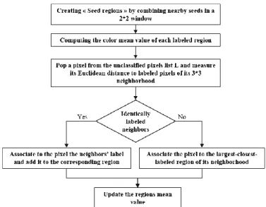
Fig.1 is a flowchart that describes the different steps included in the region growing process. Ambiguous cases of equal E-distances to different labeled regions were handled as follows: In the case of an unclassified pixel identically distant to more than one neighboring-labeled-region, we compare the sizes of the equally distant regions. The studied pixel will take the label of the closest-larger-labeled region.
At this stage of our algorithm, the results are not quite satisfying. Because our method relies on the selection of many starting seeds, the probability of winding up with an overly segmented image is high. One common solution used with the growing processing as a following up post-processing is region merging.
C. Size and Color Based Region Merging Algorithm
As a region-based method, region merging enables the clustering of complying regions and blend them into a whole sharing the same characteristics, using one or few selected rules. In general, those rules are either targeting the removal of weak edges found in shared boundaries while enhancing the boundaries strength [17] [18], or utilizing intrinsic characteristics of the regions such as color, texture, and histogram [19] [20] [1]. Under the aim of reducing the number
Vol.3 No.4, 2019 of small unnecessary information-free regions, size and color
rules prove to be the best criteria to answer to. Each condition alone delivers good results but may induce error when merging, for instance, two small regions according to the set size threshold but majorly distinct on the color basis. Under this scope, we chose to combine both criteria to guide the merging process.
To start the merging processing, the 1st condition to be verified is the region’s size. The number of pixels among each region should be less than the set threshold of 𝑇𝑠𝑖𝑧𝑒 = 1% of the total image size. Once this condition verified, we move to the assessment of the mean color value. This step makes use of (4) or (5), depending on the studied color space, to measure the color distance between the small region and another
region. If it is found inferior to the color threshold𝑇𝑐𝑜𝑙𝑜𝑟, the two regions will be merged into a whole new region, and three parameters will be updated: size, color mean and label of the new pixels’ cluster.
D. Assessment and evaluation metrics
For performance evaluation, we targeted the three following aspects: Accuracy, the noise quality and the elapsed time. Three of the commonly used metrics were employed: the Structural Similarity Index SSIM, the Mean Square error MSE and the Peak Signal to Noise Ratio PSNR [21] [22] [23]. • Structural Similarity Index (SSIM): This metric allows the
measure of resemblance between two signals X and Y, in our case between the input and the output of our proposed SRG algorithm. SSIM uses three parameters, namely the Luminance (L), the Contrast (C), and the structure (S) [24] [25]. The same parameters are highly adapted to represent and deduce the structure of a scene. Since the human visual system is sensitive to structural information, the SSIM is a great candidate to evaluate the perceived quality of our segmentation results. Also, its reliability has been proved in past studies and its consistency found better than other image assessment metrics [26] [23]. The index is expressed as follows:
𝑆𝑆𝐼𝑀(𝑋, 𝑌) = [𝐿(𝑋, 𝑌)]𝛼. [𝐶(𝑋, 𝑌)]𝛽. [𝑆(𝑋, 𝑌)]𝛿 (7)
Where:
{
𝐿(𝑋, 𝑌) = 2𝜇𝑋𝜇𝑌+ 𝑐1 𝜇𝑋2+ 𝜇𝑌2+ 𝑐1
𝐶(𝑋, 𝑌) = 2𝜎𝑋𝜎𝑌+ 𝑐2 𝜎𝑋2+ 𝜎𝑌2+ 𝑐2
𝑆(𝑋, 𝑌) = 𝜎𝑋𝑌+ 𝑐3 𝜎𝑋𝜎𝑌+ 𝑐3
(8)
The intensity-average and the standard deviation of both images X and Y are expressed by (𝜇𝑋, 𝜇𝑌) and (𝜎𝑋, 𝜎𝑌), while (𝑐1, 𝑐2, 𝑐3) are constants and α, β and δ are nonnegative weights, set by default to 1. SSIM index varies between 0 and 1, with 1 as an indicator of high similarity and as a consequence, high accuracy.
• Mean Square Error (MSE): Represents the average of the squared intensity difference measured between distorted image, and reference image pixels [22]. MSE is another frequently used quality-evaluation-metric that carries clear, interpretable physical significations. It is computed according to (9):
𝑀𝑆𝐸 = 1
𝑀𝑁∗ ∑ ∑(𝐼𝑋(𝑖, 𝑗) − 𝐼𝑌(𝑖, 𝑗)) 2 𝑁−1
𝑗=0 𝑀−1
𝑖=0
(9)
The original and the resulted images are referred to by 𝐼𝑋 and𝐼𝑌. When the MSE index carries a close to zero value, it indicates low noise levels, and subsequently, good results.
• Peak Signal to Noise Ratio (PSNR): Related to the previous metric, PSNR is another conventional measurement operating on the image intensity. The computation of this index depends on two parameters: MSE score and d, the maximum value a pixel can take, defined by the encoding of the studied image. It is defined by the following formula:
𝑃𝑆𝑁𝑅 = 10 ∗ log 𝑑 2
𝑀𝑆𝐸 (10)
In addition to these pre-defined metrics, our method was assessed according to its running time, including all the steps concisely described in Fig.2. The two signals objected to the used metrics are the original input image and the reconstructed image from the final segmentation result.
III. STUDY CONTEXT
This work was realized under the framework of the APPHOS project aiming at employing multi-spectral-image processing techniques during the mining extraction of phosphate, in order to mark rich-phosphate-areas on the deposit.
Multispectral (MS) information presents the advantage of capturing the studied-element-reflectance over specific wavelengths across the electromagnetic spectrum. The
Vol.3 No.4, 2019 particularity of this data lies in the ineptitude of traditional
color representations to support it and as a result, limits the use of these conventional spaces in advanced applications. However, the complexity of processing the MS data, strictly related to spectral dimension multiplicity is a real obstacle to exploiting and extracting meaningful information from it. To address this problem, many studies head towards integrating pre-processing steps relying on the use of dimensionality reduction and band selection methods [26] [27]. Another interesting use of band selection methods is the possibility of displaying an image with a spectral dimension equal to n into a tri-dimensional color space, chosen based on the delivered class separability results [28] [29].
Our study falls under the perspective of allowing the selection of the best visualization color space between the RGB and the HSV representations according to a metrical evaluation of SRG segmentation results. Selecting the best-displaying option for our soil MS data is believed to have a good impact on any posterior high-level processing to be privileged.
IV. EXPERIMENTAL RESULTS AND DISCUSSION
A. Dataset and Parameters Setting:
To make the results of our study more relevant, we decided to work on an image subset retrieved from the famous Berkeley dataset [30]. 20 images were picked randomly from the dataset to ensure representability of different classes. The selected data set was not subjected to any form of preprocessing, however, to ensure uniformity of the results in terms of processing time, all the images were of the size: 322*481 pixels each. The subset was projected on both considered color representations, raising the total number of study cases tested by our algorithm to 40 images. To facilitate the referencing inside the set, we will be refereeing to HSV and RGB images by Subsets (A) and (B), respectively. The followed methodology will provide a thorough and regulated comparison of the color-spaces-outcome.
Our algorithm was developed with Matlab under a test machine endowed with Windows 10 operating system and with a processor of the family Intel(R) Core(TM) i7 CPU 2.70 GHz, and a RAM memory of the size of 8 Go.
Concerning the settings of the parameters and constants, we followed an experimental approach based on the results of repeated tests with different configurations. It was found that fixing the threshold coefficient to 0.8 in both (2) and (6) delivered a better seed selection. During the merging process, and to ensure the absence of small irrelevant regions without loss of significant information, the size threshold was fixed at 1% of the total size of the images, the equivalent of 1550 pixels. The color distance limit was established 0.05 in the set (A) merging, and 2 for the set (B).
B. Comparison within the two color models:
Fig.3 displays the stepwise results of our method on an image sample from the set (A). It is clear that the visual
quality of our SRG algorithm is very satisfying. In fact, based on our perception, both reconstructed images Fig. 3(a.4) and Fig. 3(b.4) are extremely similar to their original references Fig. 3(a) and Fig. 3(b) and the SSIM rates confirm it, with consecutive scores of 96.88% and 96.98% of accuracy. On the same images, PSNR and MSE rates were very satisfying as well: For Fig. 3(a) the scores are (PSNR; MSE) = (25.61 dB; 2.7.10−3), and (PSNR; MSE) = (28.15 dB; 1.5.10−3) are scored by Fig. 3(b). These outcome witnesses not only the absence of noise elements in the final segmentation results but also the effectiveness of the region merging post-processing phase. In fact, region merging enabled us to keep a reduced number of regions equal to 1.4% of the region growing total regions in Fig. 3(a.3), and of 3.8% on Fig. 3(b.3). This major region reduction did not cause any significant loss of meaningful information and made possible the reconstruction of plausible images.
While Fig. 3(a) presents higher texture and color complexity compared to Fig. 3(b), the metrics scores ware not accordingly affected since the variations happened on a microscopic scale. However, the impact on the running time was important and approximatively 4.5 times larger on the
Vol.3 No.4, 2019 first (4642.15s versus 1090.66 s).
Concerning the data set (B), examples of the obtained results are illustrated in Fig. 4. It is clear that during the seed selection, most seeds were concentrated in the object depicted by the images and very few were chosen to describe the background. Still the reconstructed images Fig. 4(a.4) and Fig. 4(b.4) ensured an acceptable, clear degree of faith compared to the original images, in spite of slight visible color shift and of the smoothness phenomenon that overshadowed some details. This outcome reflected on the SSIM values equal to 91.74% and 88.3% which are less than the outcome scored on the same images from the set (A) by, respectively, 5.14% and 8.58%. However, the results are still considered to be delivering acceptable accuracy rates.
Moving to the PSNR and the MSE index, the scored values were as follows: For Fig. 4(a) the scores are (PSNR; MSE) = (-23.79 dB; 239.62), and (PSNR; MSE) = (-24.05 dB; 283.14) are scored by Fig. 4(b). These concordant rates indicate that the outcomes quality was damaged by the presence of ponderous noise. Since the original images were not noisy, the logical explanation, in this case, would be the introduction of noise during the execution of our SRG algorithm possibly related to an unhindered-over-segmentation
phenomenon. Under this assumption, an evaluation of the regions-number-reduction by the region merging phase was carried on and it was found that the merging effectiveness was limited. In fact, only 24.66% of the found regions were merged in Fig. 4(a.3), and even less in the case of Fig. 4(b.3) (15.34% of merged regions). This slight impact was visually depicted by the high perceptual resemblance showcased between the region growing (Fig. 4(a.2) and Fig. 4(b.2)) and the region merging displayed results (Fig. 4(a.3) and Fig. 4(b.3)).
This minor effect of the merging process over the SRG segmentation had a major impact on the running time of the whole algorithm. The execution of the collectivity of the method steps on Fig. 4(a) took 24.54s, and the elapsed time registered by Fig. 4(b) segmentation was very close with a value equal to 20.87 s.
C. Comparison between the two color models:
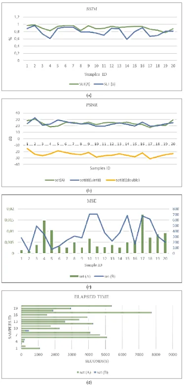
To underline the performance differences between the two studied sets (A) and (B), the quantitative results of each image, including the three used metrics scores and the time consumption aspect, were displayed in Fig. 5. According to the last, the achieved scores depends highly on the complexity and diversity of the constructional elements of each image and the impact of the color representation is clear.
Concerning the visual quality, Fig. 5 (a) shows SSIM values higher on the set (A) compared to the scores delivered by the set (B) on a total of 19 out of 20 images. On both sets the best scores was delivered by sample2, with almost 3% more resemblance ensured on the HSV color space
(𝑆𝑆𝐼𝑀𝑠𝑒𝑡(𝐴)(𝑠𝑎𝑚𝑝𝑙𝑒2) = 98.78% and
𝑆𝑆𝐼𝑀𝑠𝑒𝑡(𝐵)(𝑠𝑎𝑚𝑝𝑙𝑒2) = 96% ).While the difference between
the best scores isn’t striking, the gap between the lowest scores is very important. The lowest SSIM score among the set (A) is 77.14%, which represents a lead by 18.46% compared to the set (B) lowest score (58%). The complexity of the image seems to have more effect on the SRG segmentation product and create more confusion when projected on the RGB color space.
PSNR and MSE rates over the whole studied sets showcase divergent results as displayed in Fig. 5(b) and Fig. 5(c). On the subset (A), all the images scored high positive PSNR results, variating from a minimum equal to 17.57 dB to a maximum of 30.43 dB. Since all the scores are positive, our SRG algorithm is clearly performant on HSV images and the distortion between the reconstructed image and the original reference is minimal. Consecutively, MSE rates of the same set are very low and coherent to (10): The error rate on all the images from the set (A) is at the scale of 10−2 and less, announcing high quality of the reconstructed images and reduced noise percentage.
On the other hand, all the PSNR and MSE scores delivered by the subset (B) indicate little quality and an imposing noise presence. Fig. 5(b) demonstrates negative PSNR values on all set (B) images when encoded as “double” (d-value in (10) equal to 255), similarly to the type of encoding followed for the set (A). Changing the encoding type to “uint8” gave good
Fig. 4. Seeded region growing segmentation results on two sample images from subset (B): (a)(b) original images,(a.1)(b.1) seed selection,(a.2)(b.2) region growing, (a.3)(b.3) region merging and (a.4)(b.4) reconstructed RGB images
Vol.3 No.4, 2019 PSNR values, falling in the range of the ones found on the set
(A). This outcome insinuates the valuable impact of the encoder on the quality of our SRG algorithm when applied to RGB images, and adds another parameter to the evaluation equation. However, since the aim of our comparative study is to focus on color-aspect-influence on the segmentation results, we will be limiting our analysis to the “double” encoding type.
MSE indexes of set (B) images agree with the previous-metric-values with the scoring of very high MSE rates,
reaching a maximum of 711.82 on sample11. These results converge towards the same conclusion as the PSNR index, assuming that consistent amount of noise has been introduced during the segmentation process which had a notable effect on the final outcome.
The last aspect over which we compared the performance of our method on both subsets (A) and (B) is the elapsed time. Fig. 5(c) underline huge time consumption on the first set compared to the second with respective maximum values of 7730.05s and 143.09s. The large time utilization noticed on HSV images agrees with the analysis made in V.B, linking the large running time to computations and iterations made to reduce region’s number on this model by an average of 90%, and still provide highly accurate results while preserving fine details.
The performances averages on both studied color spaces are represented in Table IⅠ. In general, the overall accuracy scored on the HSV model is 10% better compared to the RGB model as underlined by the SSIM index. On the sets (A) and (B), MSE index scores fall in different scales, of the order of 10−3o the first (5. 10−3), and the order of 103 on the second (362.14). PSNR mean values are congruent, with respective scores of 23.83 dB and –24.37 dB. Another main difference is noticed on the running time averages, since HSV model consumes, in average 60 times more than the RGB model.
Compared to previous works, precisely to the singular color plane SRG segmentation iterating over each RGB color channel separately [15], our adapted version delivered results with better quality and visual precision while reducing the average time ( an average elapsed time of 215.92s is found on the mentioned study counter 35.04s found by our algorithm). However, the need for an adaptation to reduce the quantity of the introduced noise is imposing.
D. Noise effect attenuation:
According to the analysis conducted in V.B andin V.C, one of the reasons behind the noisy output of our SRG algorithm on RGB images is the insufficiency of the region merging step to eliminate the majority of small-meaning-free regions. Fig. 6(b) is an example of a noisy reconstructed image. It shows the presence of noise that affects even the visual quality of the image and gives an effect similar to the salt and pepper noise.
Our proposition is to add another processing block, posterior to the region merging phase, where filters will be applied only to the channel mostly impacted by the noise, measured by MSE index. Once the root-noisy-channel
TABLEII
AVERAGE PERFORMANCE EVALUATION OF THE SEGMENTATION ALGORITHM
OVER SUBSET (A) AND (B)
Subset SSIM (%) PSNR (dB) MSE Elapsed Time (s)
(A) 90.58 23.83 0.005 2657.1
(B) 80.12 -24.37 362.14 35.04
Fig. 5. Performance scores of set (A) and (B) according to SSIM (a), PSNR (b), MSE (c) and Elapsed time (d). Major differences are noticed over the PSNR, the MSE and the Elapsed time results.
Vol.3 No.4, 2019 detected, it will be subjected to a median filter before
reconstructing the final image, to be compared to the original reference.
In 50% of our sample images, the highly damaged channel was the Blue channel, 25% of the cases was the Red channel, and the left 25% the Green channel. A median filter with a 3*3 window, in accordance with the window’s size adopted in previous steps of our segmentation, was applied to the selected subject channel. The results are described in Table. III.
According to these results, the added targeted filter enabled an average reduction of the MSE index by almost 10%. However, the impact wasn’t valuable as it didn’t allow the noise rates to drop to minor values and its scale is still of the order of103.. This consequence appears clearer on the PSNR average index, where the reduction of distortion was negligible (a drop of the average value by 0.03 dB).
On the other hand, adding the filtering step to the process made the reconstructed images lose in their average perceived quality by more than 3%. This is a systematic response to the median filter which eliminates details below a certain threshold, alongside the removed noise, and induces by such, a loss in the visual quality.
Overall, the HSV color representation is capable of delivering more accurate and precise results compared to the RGB representation, under the SRG implementation. This could be related to the relative-dimension-independency characteristic of the HSV color space [31] which helped deliver a seed set that accurately guided the segmentation
process. However, the running time falls short to satisfy the requirements of a fast segmentation. Over many steps of the algorithm, we have chosen fixed thresholds and predetermined parameters adequate to detect minor variations and discriminate between overlapping, confused objects. Adaptive thresholding will be required for better results and foreground selection and these modifications could be capable of reducing the iterations number and, accordingly, the elapsed time as well.
V. CONCLUSION
In this study, we have implemented our adaptation of the SRG segmentation algorithm, using both no-edgness and smoothness criteria for the seed selection process, on two types of color images: RGB and HSV. Based on visual inspection and on metrical assessment, the experimental results underline overall good segmentation outputs on both color spaces and proved the relevance of our algorithm. Region merging post processing managed to drastically reduce the effect of over-segmentation on the HSV model. However, on the RGB dataset, the noise that affected the segmentation output could not be hindered with region merging. Adding some filtering steps to the final results did reduce its impact, however further post processing may be required for optimal denoising.
The results underline also the advantages showcased by the HSV dataset, in terms of delivering more accurate, detail preserving and noise-free results, in spite of the time consumption problem. With the right modifications, it is believed that the HSV color space will be the adequate representation to use with reduced multispectral data in order to score the best discriminating segmentation results.
ACKNOWLEDGMENT
The Authors would like to acknowledge the support through the R&D Initiative – Appel à projets autour des phosphates
APPHOS – sponsored by OCP (OCP Foundation, R&D OCP, Mohammed VI Polytechnic University, National Center of Scientific and technical Research CNRST, Ministry of Higher Education, Scientific Research and Professional Training of Morocco (MESRSFC) under the project entitled *Feasibility Study of a system discriminating between phosphate and “sterile” during the mining extraction process based on multispectral analysis*, project ID: *EXT-BRZ-01/2017* .
REFERENCES
[1] Rafael C. Gonzalez, Richard E. Woods, “Chapter10: Segmentation”, in"Digital Image Processing: 3rd edition", 2008.
[2] SEZGIN, Mehmet et SANKUR, Bülent. Survey over image thresholding techniques and quantitative performance evaluation. Journal of Electronic imaging, 2004, vol. 13, no 1, p. 146-166.
[3] YANG, Jian, HE, Yuhong, CASPERSEN, John P., et al.Delineating Individual Tree Crowns in an Uneven-Aged, Mixed Broadleaf Forest Using Multispectral Watershed Segmentation and Multiscale Fitting. IEEE Journal of Selected Topics in Applied Earth Observations and Remote Sensing, 2017, vol. 10, no 4, p. 1390-1401.W.-K. Chen,
Linear Networks and Systems. Belmont, CA: Wadsworth, 1993, pp. 123–135.
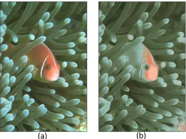
Fig. 6. An example of a noisy generated-reconstructed-image (b from the set (B)), with MSE=711.84. The image to the left (a) is the original image
TABLEIII
AVERAGE PERFORMANCE EVALUATION OF THE SEGMENTATION ALGORITHM
OVER SET (B) WITH A MEDIAN FILTER
Subset SSIM (%) PSNR
(dB) MSE
Vol.3 No.4, 2019
[4] NATH, Sumit K. et PALANIAPPAN, Kannappan. Fast graph partitioning active contours for image segmentation using histograms. EURASIP Journal on Image and Video Processing, 2010, vol. 2009, no 1, p. 820986.
[5] PANTOFARU, Caroline et HEBERT, Martial. A comparison of image segmentation algorithms. Technical Report CMU-RI-TR-05-40, Robotics Institute, Carnegie Mellon University, Pittsburgh, PA (September 2005), 2005.
[6] ADAMS, Rolf et BISCHOF, Leanne. Seeded region growing. IEEE Transactions on pattern analysis and machine intelligence, 1994, vol. 16, no 6, p. 641-647.
[7] Krishna Kant Singh, Akansha Singh, "A Study of Image Segmentation Algorithms For Different Type of Images",IJCSI International Journal of Computer Science Issues, Vol. 7, Issue 5,September 2010.
[8] Melouah, A. H. L. E. M., and R. A. D. I. A. Amirouche. "Comparative study of automatic seed selection methods for medical image segmentation by region growing technique." Recent Adv Biol Biomed Bioeng (2014): 91-7.
[9] Shweta Kansal, Pradeep Jain, "Automatic seed selection algorithm for image segmentation using region growing", International Journal of Advances in Engineering & Technology 8.3, 2015.
[10] POHLE, Regina et TOENNIES, Klaus D. Segmentation of medical images using adaptive region growing. In: Medical Imaging 2001: Image Processing. International Society for Optics and Photonics, 2001. p. 1337-1347.
[11] PATINO, Luis. Fuzzy relations applied to minimize over segmentation in watershed algorithms. Pattern Recognition Letters, 2005, vol. 26, no 6, p. 819-828.
[12] J.Fan, D.K.Y.Yau,A.K.Elmagarmid, and W.G.Aref, "Automatic image segmentation by integrating color-edge extraction and seeded region growing", IEEE Trans. Image Processing, 2001, vol.10, no.10, pp.14541466.
[13] Frank Y. Shih, Shouxian Cheng. "Automatic seeded region growing for color image segmentation", Image and Vision Computing, 2005, vol.23, pp.877-886.
[14] Huang, Liu & Li, "Color Image Segmentation by Seeded Region Growing and Region Merging", Seventh International Conference on Fuzzy Systems and Knowledge Discovery (FSKD 2010).
[15] GOTHWAL, Rajesh, GUPTA, Shikha, GUPTA, Deepak, et al.Color image segmentation algorithm based on RGB channels. In: Reliability, Infocom Technologies and Optimization (ICRITO)(Trends and Future Directions), 2014 3rd International Conference on. IEEE, 2014. p. 1-5. [16] Chaobing Huang, Quan Liu, "Color image retrieval using edge and
edge-spatial features", Chinese Optics Letters, 2006, vol.4, no.8, pp.457459.
[17] UGARRIZA, Luis Garcia, SABER, Eli, VANTARAM, Sreenath Rao, et al. Automatic image segmentation by dynamic region growth and multiresolution merging. IEEE transactions on image processing, 2009, vol. 18, no 10, p. 2275-2288.
[18] CHANG, Yu-Chou, LEE, Dah-Jye, et WANG, Yong-Gang. Color-texture segmentation of medical images based on local contrast information. In: Computational Intelligence and Bioinformatics and Computational Biology, 2007. CIBCB'07. IEEE Symposium on. IEEE, 2007. p. 488-493. [19] MEDEIROS, R. S., SCHARCANSKI, Jacob, et WONG, Alexander.
Natural scene segmentation based on a stochastic texture region merging approach. In : Acoustics, Speech and Signal Processing (ICASSP), 2013 IEEE International Conference on. IEEE, 2013. p. 1464-1467.
[20] SIMA, Haifeng et GUO, Ping. Texture Region Merging with Histogram Feature for Color Image Segmentation. In : Computational Intelligence and Security (CIS), 2013 9th International Conference on. IEEE, 2013. p. 224-228.
[21] Ren, Jianchang, et al. "Effective feature extraction and data reduction in remote sensing using hyperspectral imaging [applications corner]." IEEE Signal Processing Magazine, vol. 31, no 4, p. 149-154, 2014.
[22] Sotoca, Jos Martnez, Filiberto Pla, and Jos Salvador Sanchez. "Band selection in multispectral images by minimization of dependent information." IEEE Transactions on Systems, Man, and Cybernetics, Part C (Applications and Reviews), vol. 37, no 2, p. 258-267, 2007. [23] Su, Hongjun, Qian Du, and Peijun Du. "Hyperspectral image
visualization using band selection.", IEEE Journal of Selected Topics in Applied Earth Observations and Remote Sensing, vol. 7, no 6, p. 2647-2658, 2014.
[24] H. R. Sheikh, M. F. Sabir, and A. C. Bovik, "A statistical evaluation of recent full reference image quality assessment algorithms", IEEE Trans. Image Process., vol. 15, no. 11, pp. 3440–3451, Nov. 2006.
[25] N. Ponomarenko, V. Lukin, A. Zelensky, K. Egiazarian, M. Carli, and F. Battisti, "TID2008—A database for evaluation of full-reference visual quality assessment metrics", Adv.Modern Radio electron.,vol.10, pp. 30–45, 2009.
[26] Ren, Jianchang, et al. "Effective feature extraction and data reduction in remote sensing using hyperspectral imaging [applications corner]." IEEE Signal Processing Magazine, vol. 31, no 4, p. 149-154, 2014.
[27] Sotoca, Jos Martnez, Filiberto Pla, and Jos Salvador Sanchez. "Band selection in multispectral images by minimization of dependent information." IEEE Transactions on Systems, Man, and Cybernetics, Part C (Applications and Reviews), vol. 37, no 2, p. 258-267, 2007. [28] Su, Hongjun, Qian Du, and Peijun Du. "Hyperspectral image
visualization using band selection.", IEEE Journal of Selected Topics in Applied Earth Observations and Remote Sensing, vol. 7, no 6, p. 2647-2658, 2014.
[29] Cui, Ming, et al. "Interactive hyperspectral image visualization using convex optimization." IEEE Transactions on Geoscience and Remote Sensing, vol. 47, no 6, p. 1673-1684, 2009.
[30] The Berkley Segmentation Database and Benchmark, 2013.
https://www2.eecs.berkeley.edu/Research/Projects/CS/vision/bsds/.
[31] Chen, Wen, Yun Q. Shi, and Guorong Xuan. "Identifying computer graphics using HSV color model and statistical moments of characteristic functions." 2007 ieee international conference on multimedia and expo. IEEE, 2007.
Rajaa CHARIFI received her engineering degree in Electronics and Telecommunication from the Superior National School of Electricity and Engineering (ENSEM) in Casablanca, Morocco, in 2015. She is now pursuing her PHD studies in Signal and Image processing concerning a discriminative Analysis of phosphate during the mining extraction process using multispectral image analysis. The studies are done in the Renewable Energy and Intelligent Systems (LERSI), Faculty of Sciences and Technology (FST), University Sidi Mohammed Ben Abdellah (USMBA), Fes, Morocco.
Her major research interests include hyperspectral and multispectral remote sensing, spectral analysis, dimensionality reduction, segmentation, and classification.
Najia ES-SBAI received her PhD degree from Pau University (France) in 1993. She is a Professor in the Electric Engineering Department at the Faculty of Science and Technology, University of Sidi Mohamed Ben Abdellah (USMBA- Fez Morocco), since 1995. She completed her Ph.D. (doctorat d’état) at USMBA in 2002. She was deputy head of the electrical engineering department at the Faculty of Science and Technology of Fez for the period 2010-2013.
Vol.3 No.4, 2019 Ph.D. theses concerning the management and optimization of
energy flows in a smart grid DC isolated, intelligent inverters, DC-DC converters for energy optimization and facial expression emotion detection.
Najia ES-SBAI served about 20 committees of conference programs. She writes and co-writes more than 20 papers in national & international journals and she supervised about 50 poster and oral communications
Anass MANSOURI received his PHD degree in Microelectronics and Embedded Systems from the Faculty of Sciences and Technology (FST), Fes, Morocco, in 2009, respectively. He is an associate professor in National School of Applied Sciences (ENSA), Fes.
His major research interests include VLSI and embedded architectures design, video and image processing, as well as Software/Hardware design and optimization.
Yahya ZENNAYI received his engineer’s degree from the Faculty of Sciences and Technology (FST), Fes, Morocco, in 2013. He is now an Embedded Systems Engineer at MASCIR (Moroccan Foundation for Advanced Science, Innovation, and Research).