NUCLEI SHAPE ANALYSIS, A STATISTICAL APPROACH
A
LBERTON
ETTEL-A
GUIRREPaediatrics Department, Faculty of Medicine, University of Calgary, Room C4-435 Alberta Children’s Hospital, 2888 Shaganappi Tr. NW, Calgary, AB, T3B 6A8 Canada
e-mail: [email protected] (Accepted November 13, 2007)
ABSTRACT
The method presented in our paper suggests the use of Functional Data Analysis (FDA) techniques in an attempt to characterise the nuclei of two types of cells: Cancer and non-cancer, based on their 2 dimensional profiles. The characteristics of the profile itself, as traced by its X and Y coordinates, their first and second derivatives, their variability and use in characterization are the main focus of this approach which is not constrained to star shaped nuclei. Findings: Principal components created from the coordinates relate to shape with significant differences between nuclei type. Characterisations for each type of profile were found. Keywords: 2-dimensional profile, cancer detection, functional data analysis, principal differential analysis, star shape.
INTRODUCTION
Mitosis, the cell generating process in humans, runs at the nuclei level and, as such, there is an interest in studying the nuclei of cells with the purpose of detecting cancerous cells. Miller et al. (1994); Hobolth and Vedel Jensen (2000) indicate that the morphology of the cell nucleus will tend to be different in a healthy cell from what it is in an unhealthy cell. It is expected there would be morphological characteristics proper of cancer cells.
The study of shapes involves the imaging process step to get a “drawing” or graph, and the quantitative study of descriptors that serve the purpose of characterising such shapes. It is in the characterisation step that this paper focuses its interest.
Functional Data Analysis (FDA) (Ramsay and Silverman, 1997), a young yet growing field of statistics, offers itself as a tool in shape analysis of nuclei of cells. This tool enables the comparison of shapes without the need of strict distributional assumptions on the behaviours of the contours of nuclei. It enables the extension of known multivariate techniques such as Principal Components in the evaluation of the shapes.
In the present section, preliminaries on the statistical and biological motivation for the research, and an overview of some previous approaches are presented. The “Data and methods” section describes data preprocessing for the proposed analyses to follow; FDA using linear interpolation discussion, where Principal Components Analysis on the profiles is performed; FDA via basis functions and a curvature
based classification approach are also discussed. The last section takes advantage of the functional form of the data and its basis function approximation for an in-depth model-based analysis of the variability in the curves via Principal Differential Analysis.
When observing nuclei profiles, it is difficult to distinguish specific features or landmarks in the shape. In this sense, Miller et al. (1994) described a model for representing spatial profiles with no obvious landmarks. Recently Hobolth and Vedel Jensen (2000) have described cell nuclei as a deformable template model, their work dealt with the challenge of modeling
the process X(t). This process was modeled as a
stochastic process where, given the natural sequence or connections between points in the nucleus’ profile, the points can not be considered to be independent. Markov second order properties were imposed on the stationary cyclic stochastic process. The process was considered to be Gaussian with mean zero. The class of Gaussian process was then defined by the parameterisation of the covariance function for the process.
The deformable template model was revisited by Hobolth et al. (2002) and then the shape was modeled
with a radius-vector function and once again {X(t)}
played the role of a Gaussian residual process or deformation process.
The process{X(t)} has been presented and used to represent the continuous nucleus membrane that creates the shape or profile of such nucleus. In this sense it seems reasonable to consider the nucleus profile as a functional data source. The analyses Hobolth et al. (2002) perform are constrained to star-shaped planar objects.
The approach presented in our paper is to measure
the nucleus profile as the bivariate process Z(t) =
(X(t),Y(t)) where X(t) and Y(t) are functional
processes corresponding to the cartesian coordinates X and Y . Hence the aim is to inspect the behaviour of such processes for malignant and benign nuclei. This form of representing the profile has the advantage of not being constrained to star shaped nucleus profiles, and that the derivatives of the functional data can be computed from these, now continuous, data. Analysis on the behaviour of the derivatives sheds light on possible discriminant features that may be hidden to the naked eye.
MATERIALS AND METHODS
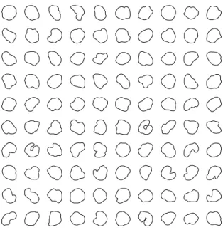
The data comprise 50 profiles of tumor cells from a benign melanocytic nevus of the human skin and 50 of malignant melanoma of the human skin. These have been studied previously in (Hobolth and Vedel Jensen, 2000), (Vedel Jensen and Sorensen, 1991), and (Gardner et al., 2005). These nuclei profiles were kindly provided by Hobolth and Jensen and can be seen in Fig. 1.
Fig. 1. ProfIles of 50 malignant cell nuclei (last 5 rows) and 50 benign cell nuclei (first 5 rows).
In our paper, the profiles were to be analysed using FDA; and in such analysis a “reference” point or time
t0 was wanted, such that it was not only meaningful
in being the first point of the nucleus profile looked at, but that would be, although arbitrary, determined by the same consistent criteria for each profile. Hence, each nucleus was fitted with an ellipse via least squares to obtain information on the rotation, if any, of such corresponding ellipse. The ellipse fitting was done via the method of Fitzgibbon et al. (1999), which is based on solving a generalised eigenvector problem.
For the analysis, where interest focuses on overall shape, the profiles are “aligned” to avoid fictitious variability. The alignment and standardisation of the profiles is obtained by rotating the profiles so that the best fitting ellipse will be resting horizontally on the semimajor axis. After being rotated, the profiles are centered and scaled so that their caliper diameter, measured parallel to the semimajor axis, ranges from −1 to 1. This standardises the range of the X
coordinates to be in[−1,1]. The Y ranges are scaled
by their corresponding X factor to preserve perspective and ratio between X and Y in each of the profiles. This normalisation is performed in the same spirit as Ramsay and Silverman (2002) do for the bone shapes and the intercondylar notch in their case study publication.
Some controversy surrounds the alignment or registration procedures. There are two main tendencies regarding shape analysis, the landmark based approach (Lele and Richtsmeier, 1991; 1992; Dryden and Mardia, 1998) and the outline based approach (Grenander and Manbeck, 1993). Our paper follows an outline based approach. Macleod (1999) states “hard distinctions between landmark and outline morphometric data/analysis are illusory and damaging to the entire enterprise of morphometrics”. The paper argues that although biological correspondence for measurements is legitimate, it does not address or avoids in itself the potential source of error. In his article it is stated that any comparison that is meaningful happens at the landmark to landmark comparison which is as good as the curve to curve comparison in comparing outlines.
It is worth mentioning that the aim of our paper is not to search for the biological reason that makes the shapes of the profiles to be the way they are. No biological homology is being assumed. Shape itself is measured as Ferson et al. (1985) do and therefore, quoting them “it is valuable to quantify shape variation sensu stricto”.
The point that will be deemed as (X(t0),Y(t0))
semimajor axis. For the linear interpolation in the profiles, measurement of the arc length starts from
t0 and t increases counterclockwise. Each profile is
represented by 150 arc-length equidistant points.
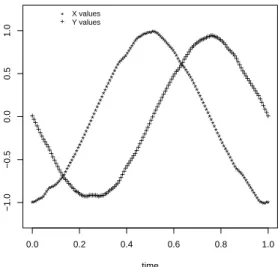
Fig. 2 shows this representation of the X(t),Y(t)
coordinates of the first benign nucleus.
0.0 0.2 0.4 0.6 0.8 1.0
−1.0
−0.5
0.0
0.5
1.0
time *********
********** ****
**** ****
**** ****
**** ****
**** ****
***** ****
************************ *****
**** *****
** **
** ****
** ****
**** *****
******* ******
********** ++
++ ++++
+++ ++
++++ ++
++++
+++++++++++++++++++++++++++++++++ ++++
++++ ++++
++++ ++++
++++ ++++
++++ +++++
++++ ++++
+++++++++++++++++++++++++ +++++
++ +++
++++++ ++++
++ ++
* + X valuesY values
Fig. 2. X(t),Y(t) for first benign nucleus based on
equidistant points.
At further stages, where derivative information is needed and analysed, the data are approximated by basis functions. Approximation for each of the
coordinates in the X(t),Y(t) process is based on
Fourier expansions for the underlying cyclic structure and on the B-spline fit for extraction of residuals information. The profiles of the nuclei are formed
by the X,Y pairs at each time t, and in this manner
each of the pairs contributes to the variability of the profile at specific positions in the profile. Based on this, the profile can be seen as having the 150 points as variables and then Principal Components Analysis can be performed to discover the type of variation that affects each of the types of profiles the most.
In order to perform PCA, each bivariate X(t),Y(t)
datum is considered separately in each of its coordinates. The data from the 100 profiles are arranged in 100 rows with 300 columns, (150 for each of X and Y coordinates) and multivariate PCA is performed on these (Ramsay and Silverman, 2002). The resulting matrix of loadings is rearranged as a three-dimensional array for easier access and interpretation. This array has in its first two dimensions
150×2 matrices of loadings for the 2-vector X,Y pairs,
and its third dimension accounts for the 100 ‘pages’ corresponding to the 100 profiles.
The purpose of performing PCA on the data is to try to detect differences in the two groups while reducing the data dimensionality. Differences in the components’ scores for the two different types of profiles are expected. Interpretability is gained from the principal components in a graphical sense by investigating the possible effect that each component has on the geometry of the mean profile.
The effect of the principal components on the shape of the profiles is captured graphically by adding and subtracting a fixed amount C times the standard deviation of the component to the mean profile
(obtained by averaging out the values of X(t),Y(t)for
each fixed t).
The effect of the first 6 principal components (accounting for 91% of variability) on the shape of the profiles is shown in Fig. 3.
PCA number 1 PCA number 2
PCA number 3 PCA number 4
PCA number 5 PCA number 6
Fig. 3. Effect of first 6 principal components on the mean profile; thick line is the mean profile, dotted line shows mean minus PCA effect and solid thin line shows mean plus pca effect.
For example, Fig. 3 shows the effect of having a component being negative or positive for profiles. The first principal component is regulating the behaviour of the convexity or concavity of the bottom part of the profile. A positive first principal component tends to make the bottom of the profile cut into the profile making it concave, whereas a negative first component tends to create a convex bump in the lower part of the profile as well as having the profile exceed the borders of the mean profile in most directions.
It is expected for benign profiles and malignant profiles to differ in the mean values on some of these components.
those of malignant cell nuclei tend to have a positive value in this component. For the second component, benign profiles tend to have negative values while malignant ones tend to have a positive value. For components 3 to 6 the benign nuclei tend to have a positive value and the malignant a negative value. It is of interest to know if these differences are significant.
Performing Welch’s T test, which is in practice fairly robust to departures form normality, on the means of each type of profile, it is seen that the mean value of the first component for benign profiles is significantly smaller than the mean value for first component of malignant profiles
(p-value < 0.002) with a 95% confidence interval
of (−1.3637,−0.2808). Wilcoxon’s rank sum test,
which does not need suffice the T test’s normality assumption, also yields a significant difference
(p-value <0.02). So the first principal component is
useful in separating benign and malignant profiles.
Means for components 2 through 5 do not show to be significantly different. However, benign profiles have a significantly higher mean for component 6 than that of the malignant profiles (Welch’s: p-value
<0.04, Wilcoxon’s: p-value<0.03)
Variability at different scales is of interest, so far, the analysis has been concerned with overall shape. The variability of the profiles at the level of their derivatives, that is, the speed at which the border of the profiles changes and comparing measures of their curvature is the next step in more detailed examination of the profiles. It is assumed that a benign cell will tend to have a smoother and convex nucleus which will have smaller total curvature measurements than that of a malignant one which is assumed that will tend to be a “squiggly”, non-convex nucleus; this curvature will be measured locally.
For example, taking the first profile from Fig. 1 (benign) and the profile in row 6 and column 7 in Fig. 1 (malignant), it is clear that the nucleus that does not “cut” into itself will have a total sum of local curvature smaller than the malignant one that is shaped like a croissant.
There is emphasis on trying methods that will measure local variability, given that, as Peura and Iivarinen (1997) discuss, some known descriptors, such as convexity ratio, prove not to be useful in distinguishing a planar object with a smooth boundary from another with irregular boundary if both happen to be non-convex. Other shape descriptors such as those explained by Gundersen et al. (1988) have been used in shape analysis as a way to condense information into simpler low-dimensional quantities, however, these
have not been created to address local differences specifically.
The nuclei are, by nature, closed curves and hence cyclic; this would suggest the use of Fourier series expansion for the profiles.
Transforming the discrete data, say zi, into
functional form (x(t)) involves representing the
function by a linear combination of a fixed number K
of known basis functions, usually denoted byφk,
x(t) =
K
∑
k=1
ckφk(t). (1)
Since interest lies in the variability of derivatives, and it is assumed that benign and malignant profiles differ on their borders locally, the fit of the basis functions was not penalised, hence the variability in the curvature was preserved rather than smoothing it out. Functional data was created based on all the observed points for each profile, but with a fixed number of basis functions to be consistent in the approximation.
A Fourier expansion with 17 basis functions was used. The choice of 17 basis functions was based on trying to capture the local variability and approximate the observed data closely. Also, when looking at boxplots of the means of coefficients of order higher than 17, these looked narrow and close to zero, therefore decided to use only 17. The Fourier approximation would be:
ˆ
x(t) =c0+c1sinωt+c2cosωt+c3sin 2ωt
+c4cos 2ωt+. . . (2)
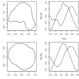
Fig. 4 shows the approximation applied to two benign profiles.
−1.0 −0.5 0.0 0.5 1.0
−0.6
−0.2
0.2
0.6
0.0 0.2 0.4 0.6 0.8 1.0
−1.0
−0.5
0.0
0.5
1.0
Time
X(t),Y(t)
−1.0 −0.5 0.0 0.5 1.0
−0.5
0.0
0.5
0.0 0.2 0.4 0.6 0.8 1.0
−1.0
−0.5
0.0
0.5
1.0
Time
X(t),Y(t)
It was observed that the means of the coefficients of order higher than 3 are not all zero which is indicative of greater deformations from elliptical templates and indicative of greater local variability existing in the profiles.
The construction of the functional form of the data guarantees that the obtained planar curve (profile) is closed and twice differentiable (Ramsay and Silverman, 1997); hence known calculus results can be used to express the profiles’ shape and curvature.
The curvatureκ(t)at some point t in the curve is:
κ(t) =X
′(t)Y′′(t)−X′′(t)Y′(t)
(X′(t)2+Y′(t)2)3/2 , (3)
and the total curvature Curv(Z) of the planar profile
takes the form:
Curv(Z) =
Z
Z
|κ(t)|dt
=
Z 1
0
|X′(t)Y′′(t)−X′′(t)Y′(t)|
X′(t)2+Y′(t)2 dt. (4)
For the calculation of curvature there is no need for registration or alignment of the data since the
integration is over the entire C2curve.
The hypothesis of interest is:
H0:µCurv(z),b=µCurv(z),m vs.
H1:µCurv(z),b<µCurv(z),m
where µi stands for the mean parameter of the
distribution of the curvatures for group i ∈ {
Malignant, Benign}.
Performing Welch’s T test it was concluded that the mean curvature of the benign profiles is
significantly smaller than that of the malignant(p=
0.00029), and performing Wilcoxon’s rank sum test
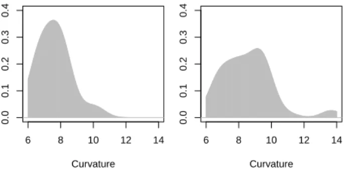
yields the same conclusion (p = 0.00067). Fig. 5
shows the density estimates for the curvatures of profiles, the curvature axis starts close to 6 as the
curvature of a closed curve C inRnis greater or equal
to 2π, with equality if and only if C is the boundary of
a two-dimensional compact convex set, as mentioned
in Proposition 2.1 of Gardner et al. (2005).
So far, the aim has been to find a process that will help to classify the profiles into malignant or benign types. Moreover, it is desirable to be able to provide some uncertainty measurement or assessment of this classification. Such a procedure should not only characterise the existing profiles, but be able to shed some light on classifying or characterising new profiles.
6 8 10 12 14
0.0
0.1
0.2
0.3
0.4
Curvature
Density
6 8 10 12 14
0.0
0.1
0.2
0.3
0.4
Curvature
Density
Fig. 5. Density estimates for the curvatures of benign (left) and malignant (right) profiles.
Hobolth et al. (2002); Hobolth and Vedel Jensen (2000) assume in their modeling, and conclude in their results, that malignant and benign profiles differ in the amount and type of variability or deformation from the templates. They also show that local variability plays a significant role in the shape of the profiles (Hobolth et al., 2003).
When creating the functional data via Fourier series, the data showed high variability at local levels. For perfectly smooth ellipses, coefficients of order higher than three would be exactly zero, because of
the parameterisation in polar coordinates: x(t) =a cost
and y(t) =b sin t for t in[0,2π]. The first 3 coefficients
would necessarily be c0 =0, c1 =0, and c2=a for
X(t); and c0=0, c1=b, and c2=0 for Y(t). There is
more structure than just that of periodical or sinusoidal
nature in the X,Y coordinates, there is also what may
be considered a residual process.
The variability structure of the coordinates can be assessed by the behaviour of their derivatives and the relationship between different orders of derivatives. Borrowing concepts from the differential equations world, a Linear Differential Operator (LDO) that determines the relationships between the derivatives of different orders is defined.
Use the following notation:
Dmx(t) = ∂
mx
∂tm , (5)
for the m-th derivative of the function x(t), where D is
the derivative operator, and when m=0 then the result
is the identity, D0x=x.
In this way, define a Linear Differential Operator by:
L=
m
∑
j=0
βjDj, (6)
Instead of assuming a homogeneous differential model, a more realistic model is assumed: a non-homogeneous system where there exists a forcing
function, sayα(t), and some error structure :
LXi(t) =αi(t) +εi(t),whereεi(t)∼N(0,σ2(t)). (7)
If the LDO captures most of the structure, the error terms are expected to oscillate very closely around zero. Given a specified LDO, it is expected for the
benign profiles to have weight functionsβi(t)different
from those of the malignant ones. Moreover, it is expected that the weight functions will characterise the type of profile.
Applying the LDO for the benign profiles (as determined by its weight functions) to a benign profile will result in a residual process as described in (7). Applying the LDO for the benign profiles to a malignant profile will give erratic residuals. Similar results will be seen if the LDO for the malignant profiles is applied to the benign and malignant types of profiles.
In order to estimate the weight functions for the operators, the data need to be registered to avoid any phase shifts that would introduce exogenous variability to the derivatives and therefore to the estimated structure.
The alignment or registration of the data is based on the creation of a “time warping” function that has the effect of stretching and/or shrinking the time
axis so that the values of Xi(t), Xj(t) for tk′ 6=tk
align according to some criterion, see Ramsay and Silverman (1997) for more details.
The mean of the benign profiles was calculated using the normalised data, that is, the 150 linearly
interpolated values of the X(t),Y(t) functions, based
on the equidistant time points for the rotated and centred profiles and this was used as a target curve for the registration.
The original rotated and centred data was then registered to this target, based on the first derivative of the data because the derivatives usually exhibit more variability and they oscillate around zero. Then the data were registered using the time warping function
(say W(t)) calculated for the derivatives.
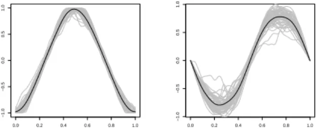
The panels in Fig. 6, show the registered X(t),Y(t)
data and the target function to which they were registered.
0.0 0.2 0.4 0.6 0.8 1.0
−1.0
−0.5
0.0
0.5
1.0
time
0.0 0.2 0.4 0.6 0.8 1.0
−1.0
−0.5
0.0
0.5
1.0
time
Fig. 6. Registered curves-gray, mean black. Left panel
X(t), right panel Y(t).
The registration procedure was done based on overall shape rather than on landmarks, otherwise, given the possible non-convexity of the profiles, the profiles would have been forced to change shape.
The global structure observed in the X(t),Y(t)
functions is of a sinusoidal nature, given this structure,
and the interest in velocity of X(t),Y(t) the linear
operator to be used, such that it would annihilate the structure of such velocity is:
Lx=D3x+β2D2x+β1Dx, (8)
which can be seen as a second order operator on the derivative of x.
This operator annihilates the structure in an exact sinusoidal structure for a homogeneous differential
system, that is to say that Lx=0, if no forcing function
is assumed to be driving the variability and if x was,
say sint. In this way : Dx=cost, D2x=−sin t, and
D3x=−cost and hence
D3x+0×D2x+1×Dx=0(β2=0,β1=1). (9)
The X(t),Y(t)functions are not exactly sint or cost
functions as they have added variability and so should
assume that there is a forcing functionαi(t)that yields
the non-homogeneous differential model as Lx=αi(t).
Let weights βj(t) for the LDO be the functions that
will characterise each type of profile.
The name of Principal Differential Analysis was coined by Ramsay as the process is, in its motivation at least, comparable to that of principal component analysis. The motivation or question is: “Can we use
a set of N functional observations xi to create a very
small set of m functions on which we can approximate efficiently the observed functions?” (Ramsay and Silverman, 1997)
In the case of the LDO, it is desired to have the LDO (defined by its weights) that comes as close as possible in satisfying the homogeneous equation
Once a decision on the operator L is taken, define
linearly independent functions, say ui, that will span
its null space. Any function x, satisfying Lx=0 can be
expressed as a linear combination of such ui.
Then minimise:
SSEPDA(L) =
N
∑
i=1
Z
[Lxi(t)]2dt, (10)
to find the weights.
The calculation of such weights is outlined in Ramsay and Silverman (1997) as these are their results.
The model for the change in X(t)being:
LX(t) =α(t) +ε(t), (11)
where
LX(t) =β1(t)DX(t) +β2(t)D2X(t) +D3X(t), (12)
and so can be expressed as
D3X(t) =β1(t)DX(t) +β2(t)D2X(t)
+α(t) +ε(t). (13)
Here, rewrite βi instead of −βi as the βi are to be
estimated.
In the calculations, estimate the forcing function
α(t), the weight functionsβ1(t),β2(t)simultaneously
and from these estimate the residual processε(t).
B-splines are useful in approximating functions with local variability, more so than Fourier series. Hence 47 B-spline basis functions of order 8 were used for creating the functional forms of the data. The order might seem high, but the reader is reminded that the aim is to calculate third derivatives with penalised smoothing for the creation of the functional data. The penalisation, as described in (Green and Silverman, 1994; Ramsay and Silverman, 1997) will be dealing with 5th order derivatives and hence the fit is done with 2 degrees more; this results in degree 7 and therefore
the order (degree of local polynomial+1) has to be 8.
The choice of 47 basis functions yields 41 knots which gives, in the case of the smallest number of points in a profile (189 points), about 5 internal points between knots, and in the case of the greatest number of points in a profile (343 points), some 8 internal points.
Six functions for the benign profiles and six for the
malignant are estimated: Two forcing functionsαX(t)
andαY(t), and the four weight functionsβ1X,β2X,β1Y,
β2Y for each type.
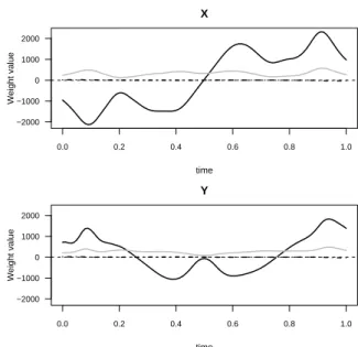
The forcing and weight functions for benign profiles are presented together in Fig. 7. It can be seen that the forcing function is the largest source of variation and how the first and second derivatives have smaller impact in such variability.
0.0 0.2 0.4 0.6 0.8 1.0
−2000 −1000 0 1000 2000
X
time
Weight value
0.0 0.2 0.4 0.6 0.8 1.0
−2000 −1000 0 1000 2000
Y
time
Weight value
Fig. 7. Forcing and weight functions for benign profiles. Solid black line is the forcing function, grey line is ˆβ1and dashed line is ˆβ2.
Residual functions obtained from applying the LDO with weights calculated from all 50 benign profiles to the benign profiles were estimated. Since the aim is to classify new profiles, such a process is mimicked by calculating the residuals for each of the benign profiles by leave one out crossvalidation.
Residual functions calculated for malignant
profiles using the weight functions from the benign profiles should be significantly greater than the ones obtained for the benign profiles using the same weight functions. The forcing and weight functions for malignant profiles are presented together in Fig. 8. It can be seen that the forcing function is the largest source of variation and how the first and second derivatives have smaller impact.
The residual functions obtained from applying the LDO with weights calculated from all 50 malignant profiles to the malignant profiles were estimated via crossvalidation as done for applying benign profiles’ weights on benign profiles.
Residual functions calculated for benign profiles using the weight functions from the malignant profiles significantly deviate from 0, more so than the ones obtained for the malignant profiles using the same malignant weight functions.
0.0 0.2 0.4 0.6 0.8 1.0 −2000
−1000 0 1000 2000
X
time
Weight value
0.0 0.2 0.4 0.6 0.8 1.0
−2000 −1000 0 1000 2000
Y
time
Weight value
Fig. 8. Forcing and weight functions for malignant profiles. Solid black line is the forcing function, grey line is ˆβ1and dashed line is ˆβ2.
Fig. 9 shows the functional 95% confidence
intervals for the X(t)and Y(t)mean residual curves of
benign on benign and of malignant on malignant and it is clear that zero is always inside the intervals.
0.0 0.2 0.4 0.6 0.8 1.0 −100
−50 0 50 100
X(t)
time CI
0.0 0.2 0.4 0.6 0.8 1.0 −150
−100 −50 0 50 100 150 200
Y(t)
time CI
Fig. 9. 95% Confidence-like interval for the mean of residuals. Black line: benign on benign, gray line: malignant on malignant.
These intervals are calculated in an analogous way as confidence intervals for point estimates, the only difference is that the mean and standard deviation of the curves are curves themselves. The standard deviation is a function of the parameter t, it varies at different times t.
Figs. 10 and 11 show the p-values for the Wilcoxon test for the location parameter of zero. These figures show that the p-value-curves for benign on benign
are not less than 0.53 for X(t) residuals and not less
than 0.33 for Y(t) for any t ∈[0,1]; the p-values for
malignant on malignant are not less than 0.21 for X(t)
and not less than 0.29 for Y(t) for any t ∈[0,1]and
hence it can be concluded that the residuals are centred
at zero at all times t∈[0,1].
0.0 0.2 0.4 0.6 0.8 1.0 0.0
0.2 0.4 0.6 0.8 1.0
X(t)
time
Pvalue
Fig. 10. Pointwise (fine grid of 1000 times ti) P-values
of testing mean of residuals (µ) equals 0 for (X ) .
Black line: benign on benign, gray line: malignant on malignant, dashed line: P-value = 0.05.
0.0 0.2 0.4 0.6 0.8 1.0 0.0
0.2 0.4 0.6 0.8 1.0
Y(t)
time
Pvalue
Fig. 11. Pointwise (fine grid of 1000 times ti) P-values
of testing mean of residuals (µ) equals 0 for (Y ).
Fig. 12 shows the functional 95% confidence
intervals for the X(t) and Y(t) mean residuals of
benign on malignant and for malignant on benign and it is clear that zero is not always inside the intervals.
0.0 0.2 0.4 0.6 0.8 1.0 −200
−100 0 100 200
X(t)
time CI
0.0 0.2 0.4 0.6 0.8 1.0 −200
0 200 400
Y(t)
time CI
Fig. 12. 95% Confidence-like interval for the mean of residuals. Black line: benign on malignant, gray line: malignant on benign.
Figs. 13 and 14 show the p-values for the Wilcoxon test for the location parameter of zero. This figure
shows that the p-values are less than 0.05 in some
intervals, and in those time periods it can be concluded that the residuals are centred at a value significantly different from zero.
0.0 0.2 0.4 0.6 0.8 1.0 0.0
0.2 0.4 0.6 0.8 1.0
X(t)
time
Pvalue
Fig. 13. Pointwise (fine grid of 1000 times ti) P-values
of testing mean of residuals (µ) equals 0 for (X ). Black
line: benign on malignant, gray line: malignant on benign. Dashed line: P-value=0.05.
0.0 0.2 0.4 0.6 0.8 1.0 0.0
0.2 0.4 0.6 0.8 1.0
Y(t)
time
Pvalue
Fig. 14. Pointwise (fine grid of 1000 times ti) P-values
of testing mean of residuals (µ) equals 0 for (Y ). Black
line: benign on malignant, gray line: malignant on benign. Dashed line: P-value=0.05.
The analysis has shown that the residual processes obtained by applying weight functions of the same type as the profile type (benign on benign or malignant on malignant) are “well behaved” in both of the
coordinates X,Y and their confidence intervals always
cover zero. On the other hand, when applying weight functions of different type than that of the profiles (benign on malignant, malignant on benign) the residual processes are “ill behaved” in at least one of
the coordinates X,Y , having the confidence intervals
not covering zero over non-negligible proportions of
time spanning from 21.1% to 52.5%.
Based on this analysis and given the fact that profiles are obtained in batches, say from a biopsy, a new batch of profiles can be digitised, converted into functional data, registered to the benign profiles’ mean function and then have the weight functions applied to each of the profiles to obtain the residual processes. Once these are obtained, the confidence intervals and/or the Wilcoxon tests can be performed to obtain a diagnostic of benign or malignant.
CONCLUSION
The alignment and registration of the profiles is, from a biological point of view, arbitrary and has no physiological meaning. It is, however, a protocol followed to analyse all profiles in a consistent way. The ‘reference’ point is reached in each profile by following a fixed criterion.
The ways in which the methods were applied in this paper allowed dealing with the profiles as continuous functions which better represent the continuous form and nature of the nuclei profiles, and without the restriction to objects that are star shaped with respect to their centre of mass as in (Hobolth et al., 2002).
Excluding the non-star shaped profiles from the present data could have affected the discovery of the characteristics pointed out by the first principal component, as in that analysis it is seen that one of the graphical characteristics where the scores of principal components differ significantly relates to the non-convexity of the shape and the non-star shaped profiles in this data set also happened to be non-convex.
This paper shows in a tangible graphical way, the shape differences between the two types of profiles. A useful tool in the principal differential analysis gave the criterion for classification based on the behaviour of 95% intervals for the residuals. When it comes to having some measure of uncertainty, the reader could relate to the confidence intervals and the p-value function. It is important that the reader remembers that the profiles, although they are presented individually, belong to a set of nuclei which comes from one tissue sample such as a biopsy. In this sense, an analyst will not be facing the problem of having only one profile to diagnose or to classify, as there will be a set of profiles and hence the sample means and standard deviations of the residuals obtained by applying the weight functions, and so, the construction of the confidence intervals is possible.
REFERENCES
Dryden I, Mardia K (1998). Statistical shape analysis. Wiley.
Ferson S, Rohlf F, Kohen R (1985). Measuring shape variation of two-dimensional outlines. Syst Zool 34:59– 68.
Fitzgibbon AW, Pilu M, Fisher RB (1999). Direct least-squares fitting of ellipses. IEEE Trans Pattern Anal 21:476–80.
Gardner R, Hobolth A, Jensen E, Srensen F (2005). Shape discrimination by total curvature, with a view to cancer diagnostics. J Microsc 217:49–59.
Green P, Silverman B (1994). Nonparametric Regression and Generalized Linear Models (A roughness penalty approach). London: Chapman & Hall, 1st ed.
Grenander U, Manbeck K (1993). A stochastic model for defect detection in potatoes. J Comput Graph Stat 2:131–51.
Gundersen HJG, Bendtsen TF, Korbo L, Marcussen N, M11er A, Nielsen K, Nyengaard JR, Pakkenberg B, Srensen FB, Vesterby A, West MJ (1988). Some new, simple and efficient stereological methods and their use in pathological research and diagnosis. Acta Path Micro Im 96:379–94.
Hobolth A, Pedersen J, Vedel Jensen E (2002). A deformable template model, with special reference to elliptical templates. J Math Imaging Vis 17 (2):131–7. Hobolth A, Pedersen J, Vedel Jensen E (2003). A continuous
parametric shape model. Ann I Stat Math 55:227–42. Hobolth A, Vedel Jensen E (2000). Modelling stochastic
changes in curve shape, with an application to cancer diagnostics. Adv Appl Probab 32:344–62.
Lele S, Richtsmeier J (1991). Euclidean distance matrix analysis: A coordinate free approach for comparing biological shapes using landmark data. Am J Phys Anthropol 86:415–27.
Lele S, Richtsmeier J (1992). On comparing biological shapes: Detection of influential landmarks. Am J Phys Anthropol 87:49–65.
Macleod N (1999). Generalizing and extending the eigenshape method of shape space visualization and analysis. Paleobiology 25:10–138.
Miller M, Joshi S, Maffitt D, McNally J, Grenander U (1994). Membranes, mitochondria and ameoba: shape models. Adv Appl Stat II:141–63.
Peura M, Iivarinen J (1997). Efficiency of simple shape descriptors. In: Proceedings from the Third International Workshop on Visual Form.
Ramsay J, Dalzell C (1991). Some tools for functional data analysis. J Royal Stat Soc B 53:539–72.
Ramsay J, Silverman B (1997). Functional Data Analysis. New York: Springer-Verlag.
Ramsay J, Silverman B (2002). Applied Functional Data Analysis,methods and case studies. New York: Springer-Verlag, 1st ed.