Disk Resident Taxonomy Mining for Large Temporal Datasets
P.Lakshmi Bhanu1, Mrs. N.Leelavathy2,, Mrs.G.Satya Suneetha2 M.Tech Student1, Professor & HOD2, Associate Professor3
Department of Computer Science & Engineering, Pragati Engineering College[1,2,3] East Godavari (dt), A.P,India
Abstract
Mining patterns under constraints in large data is a significant task to advantage from the multiple uses of the patterns embedded in these data sets. It is obviously a difficult task because of the exponential growth of the search space. Extracting the patterns under various kinds of constraints in such type of data is a challenging research. First, a memory-based, efficient pattern-growth algorithm, Forest Mine, is proposed for mining frequent patterns for the data sets and then consolidating global frequent patterns. For dense data sets, Forest-mine is integrated with FP-Tree dynamically by detecting the swapping condition and constructing FP-trees for efficient mining. Such efforts ensure that forest mine is scalable in both large and medium sized databases and in both sparse and dense data sets.
Index Terms: Frequent Generalized Item Set,
FP-Tree,Forest Mine, Disk Resident Data structure
Introduction
Mining frequent data sets is a common problem for mining association rules. It also plays an important role in many data mining tasks like sequential patterns, episodes, multi-dimensional patterns and so on. The description of the problem is as follows. Let I ={i1,
i2, . . . , in}, be a set of items. Items will sometimes also be denoted by a, b, c, . . .. An I-transaction τis a subset of I. An transactional database D is a finite bag of I-transactions. The support of an itemset S ⊆ I is the
proportion of transactions in D that contain S. The task of mining frequent itemsets is to find all S such that the support of S is greater than some given minimum
support ξ, where ξ either is a fraction , or an absolute count. Most of the algorithms, such as Apriori, DepthProject, and dEclat work well when the main memory is big enough to fit the whole database or/and the data structures (candidate sets, FP-trees, etc) [1]. When a database is very large or when the minimum support is very low, either the data structures used by the algorithms may not be accommodated in main memory,
or the algorithms spend too much time on multiple passes over the database. In the First IEEE ICDM Workshop on
Frequent Itemset Mining Implementations, FIMI ’03, many well known algorithms were implemented and
independently tested. The results show that “none of the
algorithms is able to gracefully scale-up to very large datasets,with millions of transactions”[1].
At the same time very large databases do exist in real life. In a medium sized business or in a
company big as Walmart, it’s very easy to collect a few
gigabytes of data. Terabytes of raw data are ubiquitously being recorded in commerce, science and government. The question of how to handle these databases is still one of the most difficult problems in data mining[2].
In the paper [1] authors considered the problem of mining frequent itemsets from very large databases. They adopt a divide-and-conquer approach. First they presented three algorithms, the general divide-and-conquer algorithm, then an algorithm using basic projection (division), and an algorithm using aggressive projection. They also analyzedthe disk I/O’s required by
those algorithms. In a detailed divide-and-conquer algorithm, called Diskmine, they use the highly efficient
FPgrowth* method to mine frequent itemsets from an
FP-tree for the main memory part of data mining. We describe several novel techniques useful in mining frequent itemsets from disks, such as the FP-array technique, and the item-grouping technique.
Existing System
There have been many algorithms developed for fast mining of frequent patterns, which can be classified into two categories. The first category, candidate generation and test approach, such as Apriori as well as many subsequent studies, are directly based on an anti-monotone Apriori property if a pattern with k items is not frequent, any of its super-pattern with (k+1) or more items can never be frequent[3].
Limitations of Existing Systems
Real data sets can be sparse and/or dense in different applications
3. Third, large applications need more scalability. Many existing methods are efficient when the data set is not very large. Otherwise, their core data structures (such as FP-tree) or the intermediate results (e.g., the set of candidates in Apriori or the recursively generated conditional databases in FP-growth) may not fit in main memory and easily cause thrashing
Problem Statement
The problem of frequent pattern mining is to find the complete set of frequent patterns in a given transaction database with respect to a given support threshold
Proposed Work
This study is proposing a forest data structure, and a mining algorithm, Forest-mine, which takes advantage of this data structure and dynamically adjusts links in the mining process. A divergent feature of proposed method is that it has very restricted and precisely banal space overhead and runs truly rapid in memory-based setting. Moreover, it can be extended up to very large databases by database segregation, and when the data set becomes impenetrable, FP-trees can be built dynamically in the mining.Tackle the problems of mining in dynamic large data base. This is a challenging task that requires extending disc resident FP-Tree into a dynamic structure that could smoothly absorb modifications to the database.
Mining from disk:
How should one go about when mining frequent item-sets from very large databases residing in a
secondary memory storage, such as disks? Here “very large” means that the data structures constructed from the
database for mining frequent item-sets can not fit in the available main memory. One approach is sampling.. Unfortunately, the results of sampling are probabilistic; some critical frequent item-sets could be missing. Besides the sampling, there are basically two strategies for mining frequent item-sets, the data structures approach, and the divide-and-conquer approach. The
data structures approach consists of reading the database
buffer by buffer, and generates data structures (i.e. Candidate sets or FP-trees). Since the data structure do not fit into primary memory, supplementary disk I/O’s
are required. The number of passes and disk I/O’s
required by the approach depends on the algorithm and its data structures.
For examples, if the algorithm is Apriori using a hash-tree for candidate itemsets, disk based hash-trees have to be used. If the algorithm is FP-growth method, as suggested, FP-trees have to be written to the disk. Then
the number of disk I/O’s for the trees depends on the size
of the trees on disk. Note that the size of the trees could be the same as or even bigger than the size of the database. The basic strategy for the divide-and-conquer approach is shown in the procedure diskmine. In the approach, |D| denotes the size of the data structures used by the mining algorithm, and M is the size of available main memory. After all small databases are processed, all candidate frequent itemsets are combined in some way (obviously depending on the way the decomposition was done) to get all frequent itemsets for the original database.
Procedure diskmine(D,M) if |D| ≤ M then return mainmine(D) else decompose D into D1, . . .Dk. return
combine diskmine(D1,M),.... , diskmine(Dk,M). The efficiency of diskmine depends on the method used for mining frequent itemsets in main memory and on the
number of disk I/O’s needed in the decomposition and
combination phases. Sometimes the disk I/O is the main factor. Since the decomposition step involves I/O, ideally the number of recursive calls should be kept small. The faster we can obtain small decomposed databases, the fewer recursive call we will need. On the other hand, if a decomposition cuts down the size of the projected databases drastically, the trade-off might be that the combination step becomes more complicated and might involve heavy disk I/O. In the following we discuss two decomposition strategies, namely decomposition by partition, and decomposition by projection. Partitioning is an approach in which a large database is decomposed into cells of small non-overlapping databases. The cell-size is chosen so that all frequent itemsets in a cell can be mined without having to store any data structures in secondary memory. However, since a cell only contains partial frequency information of the original database, all frequent itemsets from the cell are local to that cell of the partition, and could only be candidate frequent itemsets, for the intact dataset. Thus the contestant frequent itemsets mined from a unit have to be demonstrated later to filter out false hits. Consequently, those candidate sets have to be written to disk in order to leave space for processing the next cell of the partition.
After generating candidate frequent itemsets from all cells, another database scan is needed to filter out all infrequent itemsets. The segregation approach therefore needs only two passes over the dataset, but inscription and interpretation candidate frequent itemsets will involve a momentous number of
disk I/O’s, depending on the range of the set of contestant
of this approach is that any frequent item set mined from a anticipated database is a frequent itemset in the imaginative database. To get all frequent item sets, only need to take the unification of the frequent item sets discovered in the small anticipated databases. The biggest problem of the bulge approach is that the total size of the projected dataset could be excessively large, and there could be excessively many disk I/O’s for the
projected datasets. Thus, there is a tradeoff between the easier amalgamation segment and possible excessive
many disk I/O’s. To analyze the recurrence and required disk I/O’s of the general divide-and-conquer algorithm when the putrefaction stratagem is projection.
Definition 1 Let I be a set of items. By I∗we will enote
strings over I, such that each symbol occurs at most once
in the string. If α, β are strings, then α.β denotes the concatenation of the stringαwith the string β. Let D be an I-database. Then FI(D) is the string over I, such that each frequent item in D occurs in it precisely once, and the items are in non-increasing order of frequency in D. As an example, consider the {a, b, c, d, e}-database D =
{{a, c, d}, {b, c, d, e}, {a, b}, {a, c}}. If the minimum
support is 50%, then freqstring(D) = acbd.
Definition 2 Let D be an I-database, and let FI(D) = i1i2
・ ・ ・ik. For j∈{1, . . . , k} we define Dij = {τ ∩ {i1, .
. . , ij} : ij ∈ τ, τ ∈ D}. Let α ∈ I∗. We define Dα inductively: D’= D, and let FI(Dα) = i1i2 ・ ・ ・ ik. Then, for j∈{1, . . . , k}, Dα.ij= {τ ∩ {i1, . . . , ij} : ij∈
τ, τ∈Dα}. Obviously, Dα.ijis an {i1, . . . , ij} -database. The putrefaction of Dαinto Dα.i1, . . . , Dα.ikis called the
basic estimate. To illustrate the basic estimate, from
earlier example, starting from the least frequent item in the FI, one can obtain Dd = {{a, c, d}, {b, c, d}}, Db =
{{c, b}, {a, b}}, Dc = {{a, c}, {c}, {a, c}}, and Da = {{a}, {a}, {a}}.
Definition 3 Let α ∈ I∗, ij ∈ I, and let Dα.ij be an I database. Then FS(ξ,Dα. ij) denotes the subsets of I that contain ij and are frequent in Dα. ijwhen the minimum support isξ. Usually, we shall abstractξaway, and write just FS(Dα. ij).
In the previous example, for Dd, FS(Dd)={{d},
{c, d}}. Note though {c} is also frequent in Dd, it is not listed since it does not contain d. It will be listed in
FS(Dc). Similarly, FS(Db)={{b}}, FS(Dc)={{c}, {a, c}} and FS(Da)={{a}}. We also can notice that Ddand Dcare not that much smaller than the original database. The upside is though that the set of all frequent itemsets in D now simply is the union of FS(Dd), FS(Db), FS(Dc) and
FS(Dd). This means that the combination phase is a simple union. The following procedure BDM gives a divide-and-conquer algorithm that uses basic projection. A transactionτin Dαwill be partly inserted into Dα. ijif and only if τ contains ij . The parallel projection algorithm introduced an algorithm of this kind.
Procedure BDM(Dα,M)
if |Dα|≤M then return mainmine( Dα)
else let FI(Dα) = i1i2・ ・ ・in,
return DISKMINE(Dα. i1,M)∪. . .∪BDM(Dα. in,M).
Let’s analyze the disk I/O’s of the algorithm
BDM. As before, we assume that there are two passes,
that the data structure is an FP-tree, and that the main memory mining method is FP-growth. If in D’, each transaction contains on the average n frequent items, each transaction will be written to n projected databases. Thus the total length of the associated transactions in the projected databases is n+(n−1)+・ ・ ・+1 = n(n+1)/2, the total size of all projected databases is (n+1)/2・D≈
n/2・D. Still there are two full database scans and a
incomplete database scan for D’, as explained for
formula (1). The number of total disk I/O’s is 5/2・D/B.
The projected databases have to be written to the disks first, then later scanned twice each for building an FP-tree. This step needs at least 3・ n/2 × D/B. Thus, the
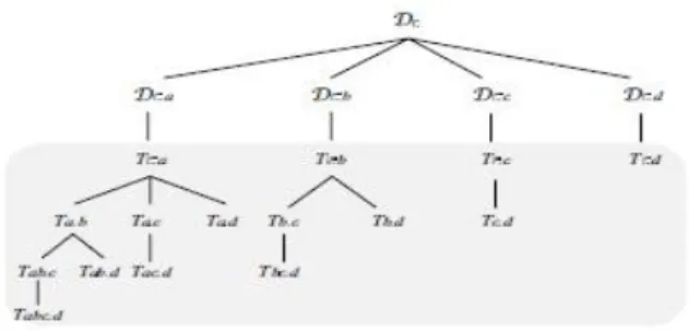
total disk I/O’s for the divide-and-conquer algorithm with basic projection is 5/2・D/B + n・3/2・D/B (2) The
recurrence structure of BDM is shown in Figure 1. The reader should ignore nodes in the shaded area at this point, they represent processing in main memory.
In a typical application n, the average number of frequent items could be hundreds, or thousands. It therefore makes sense to devise a smarter projection strategy. Before we go further, we introduce some definitions and a lemma.
Generalized Itemset Discovery: The rules that are
generated by support and confidence are difficult to analyse which is called Association rule extraction, even if their buried data might be relevant. To analyse
similarities between data’s are done by powerful and
effective tools where even some buried information are extracted by previous approaches. The objective is to monitor tactic that balance the data immoderation load and better utilize a multi-core cluster system for data mining application. The main issue in this paper is low
performance. It won’t mine all frequent generalizations
of an atypical pattern, but slightly generates only the one characterized by low redundancy
2) Change Detection in Datasets: This paper presents a
sketch out to detect changes inside a data set at imaginary level very deeply. The main idea is to obtain a rule-based illustration of the data set at different time period and to rarely analyze how these regulations change. Discovering changes and acting upon to or them or before any other item-set others has become a tenaciously issue for many organization. Prevailing data analysis practices shows that task under contemplation is steady over number of times due to conjecture. Here exposure and mutable are made at imaginary level only it may not be real or true. The main shortcoming is conferred previously. Pretend may sometimes workout but not all the time. The detection, based on real dataset should be made to get accurate result
3) Frequent Generalized Item Sets: FGIS takes input as
pecking order. Then classify it and harvests generalized item-set by using association rules which happens same in generalized item-set. The results generated by using association rules are strongly recommended by users not automatically generated. The FGIS algorithm amends and conglomerates result produced by two algorithms. The result encloses unordered item-sets. These algorithms extract item-set by processing transactional database. FGIS+ The shortcoming in FGIS is recovered by FGIS+. It is proficient and solves numerous problems of pattern extraction, such as the expensive creation of Training date set sets and the over-generalization of rules. Item set parallelism in multiprocessing and multi-computing state is analyzed in this paper. Another important drawback isload balancing, this is also recovered. But the drawback in FGIS + is dynamic load balancing where both candidate set and computation task are handled.
Load Items
The Load items will load the items from the database for the mining task is to discover a set of attributes shared among a large number of objects in a given database.
Load Transaction
This transactional database, first scan the database once to collect the count of the items present in the database. Then, sort the items according to their frequencies in descending order to build the frequent item list. Only items those come across the minimum support threshold are deliberated for building the FP-tree. All items are carried out with their support counts.
Load next window
It performs a second scan of the transactional database to build the FP-tree. Begin with an empty root and add the transactions one-by-one as prefix subtrees of the root. After reading each transaction, sort its items in descendant order by the support.
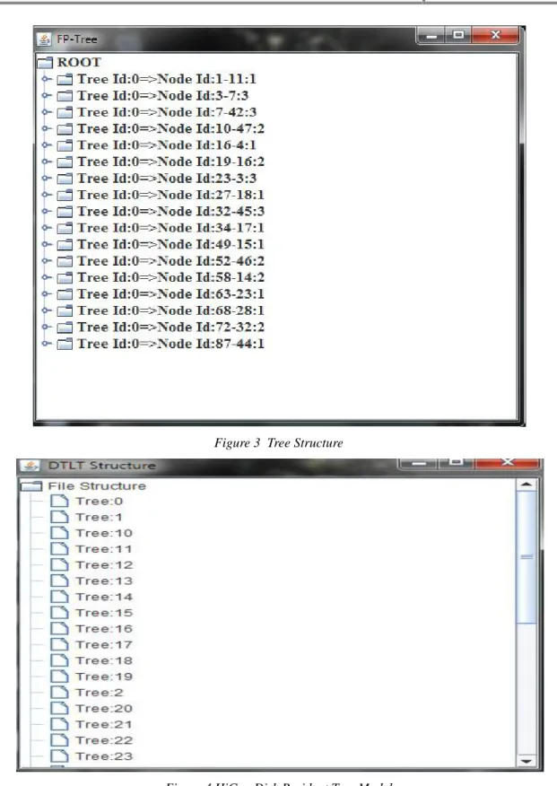
Build Tree
This subunit builds in memory the initial FP-tree from the raw data files. The transactions are read from the file one-by-one; and they are added to the tree which is realized in the nodes-list. Management of the FP-nodes-list is done by MMU which keeps track of the free and already occupied nodes of the list. While constructing the FP-tree in M.B, this subunit may consult the tree translation unit of MMU in order to translate part of the current tree into secondary storage system S; this will make room for the new FP-nodes corresponding to the transactions to be added next. After the translation process, the tree construction will resume to use FP-nodes by assuming that no part of the tree is present in main memory. Here, it is worth mentioning that the effect of this tree translation process will lead to the situation as if the initial tree has been constructed as separate chunks of trees. Consequently, the complete set of truncated transactions of the database will be represented by these chunks of trees and the mining result will not be affected. However, the database will not be as compressed as the original FP-tree because multiple paths sharing same prefix
SaveTree
The ‘Build Tree from the Database’ subunit, it may find that there is not enough space available in ‘FP
-Nodes list’ to continue the tree building process and may
portion of the tree by breaking out of the loop. We require the lastTree variable because this memorizes the point at which we break out from the loop. For items with ids > lastTree, we still need to traverse that portion of the base tree which was just saved in the secondary storage
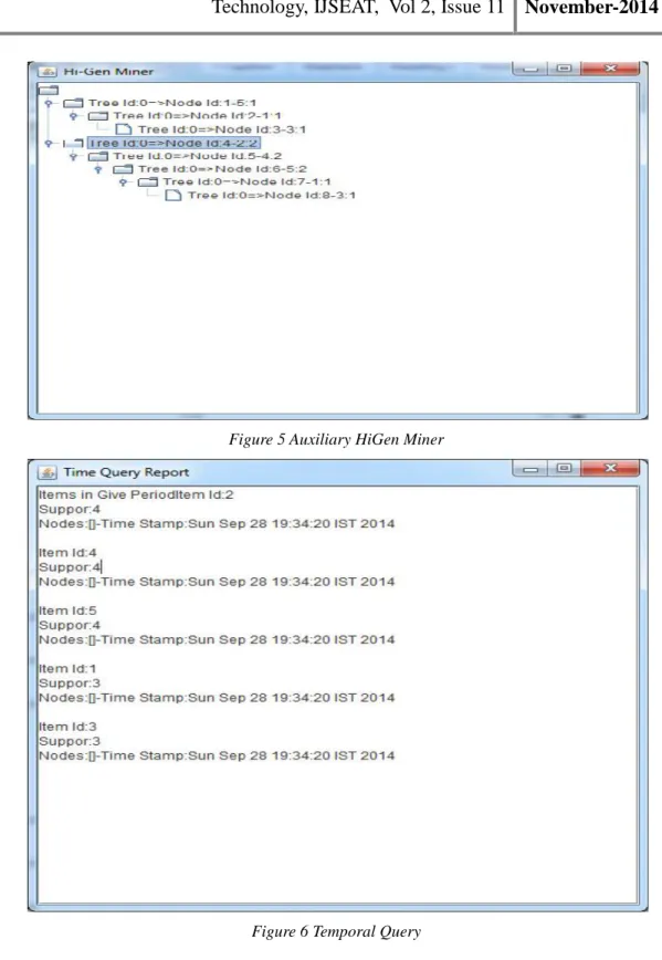
DTLT Structure
Disc Tree Location Table (DTLT) is an R-tree based structure that stores the knowledge of Prefix-Treediscnode-Id ranges associated with each prefix-tree in order to facilitate easy lookups of the blocks that constitute a particular Prefix-Treedisc as a disc file. The DTLT structure gets affected when the tree translation
unit translates some of the FP-trees from memory to I/O-conscious prefix-trees, which are all represented in a single file-based structure. At any stage of the mining process, multiple FP-trees might be available in memory. The mining model may need to make room in the available memory
space M.B by translating some of the FP-trees into disc-based I/O-conscious prefix-trees; this is realized in multiple blocks, where each block size is less that the size of FB in order to be accommodated in FB at a later stage. Subsequently, the mining model also inserts block location data for a particular prefix-tree into DTLT structure
Results
Figure 3 Tree Structure
Figure 5 Auxiliary HiGen Miner
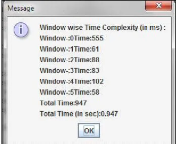
Figure 7 Time Complexity
References
[1] Mining Frequent Itemsets from Secondary Memory, G¨osta Grahne and Jianfei Zhu, Concordia University,Montreal, Canada
[2] “Mining Frequent δ-Free Patterns in Large Databases”,Céline Hébert, Bruno Crémilleux, Discovery Science,Lecture Notes in Computer Science Volume 3735, 2005, pp 124-136