Performance Modeling of
Delay-based Dynamic Speed Scaling
Systems
Caglar Tunc
Nail Akar
[email protected]
[email protected]
Bilkent University
Deparment of Electrical and Electronics Engineering
Ankara, Turkey
Performance Modeling of Delay-based Dynamic Speed Scaling 2
Outline
•
Introduction
•
Problem Definition
•
Markov Fluid Queues
•
Delay-based Dynamic Speed Scaling Model
•
Numerical Examples
Performance Modeling of Delay-based Dynamic Speed Scaling 3
Single Server Speed Scaling
•
Speed scaling
: Adapting the speed of a computer or
communication system to tradeoff energy and
performance
i. Static speed scaling
: System is busy
⇒
single speed,
System is idle
⇒
sleep mode
ii. Dynamic speed scaling
: Speed is continuously adapted
based on the system state, i.e., the number of jobs in the
system, delay experienced by jobs, etc.
Performance Modeling of Delay-based Dynamic Speed Scaling 4
Single Server Speed Scaling
•
Low speed
↔
low power
•
Takes longer to finish a task with lower speed, BUT
generally less energy is consumed
•
How to adapt the speed according to the system state
[1]
[2]
.
F. Yao, A. Demers, and S. Shenker. A Scheduling Model for Reduced CPU Energy
. In Proceedings
of FOCS '95
, pages 374-, Washington, DC, USA, 1995. IEEE Computer Society.
C. Gunaratne, K. Christensen, B. Nordman, and S. Suen. Reducing the Energy Consumption of
Ethernet with Adaptive Link Rate (ALR).
Computers, IEEE Trans on
, 57(4):448-461, April 2008.
Motivating Application Areas
o
Adaptive speed in processors and computer systems
Change the speed of a processor according to the number
of jobs waiting in the system to save energy
[1]
o
Adaptive link rate (ALR) schemes in Ethernet links
Change the rate of an Ethernet link according to the link
utilization to obtain energy savings (not standardized)
[2]
Data rate =
�
100
Mbps,
if link utilization
<
10%
Performance Modeling of Delay-based Dynamic Speed Scaling 6
Motivating Future Applications
o
Wireless link that supports different power levels and
adaptive coding and modulation (ACM) techniques
o
Adjust the link rate according to delays of the jobs in the
system
Performance Modeling of Delay-based Dynamic Speed Scaling 7
Delay-based Dynamic Speed Scaling
•
Assign a service rate for the head-of-the-line (HOL) job of a
FIFO queue according to the total delay it has experienced
in the system
•
Jobs may have strict deadlines
Jobs with delays greater than the deadline abandon the
system without service
Performance Modeling of Delay-based Dynamic Speed Scaling 8
Markov Fluid Queues (MFQs)
•
Background process determines the rate of change (
drift
) of a
buffer
•
Finite state space Continuous Time Markov Chain (CTMC)
•
Each state has its own drift value
•
Infinitesimal generator and drift values
•
Multi-Regime (Multi-Layer/Multi-Threshold) MFQ (MRMFQ)
Buffer is divided into a finite number of regimes
Sample Evolution of an MRMFQ
1
2
Time
State 1
Regime 1
State 1
Regime 2
State 2
Regime 2
State 2
Regime 1
𝑿𝑿
(
𝒕𝒕
)
𝑻𝑻
(
𝟐𝟐
)
=
𝑩𝑩
𝑻𝑻
(
𝟏𝟏
)
𝒖𝒖
𝑻𝑻
(
𝟎𝟎
)
=
𝟎𝟎
[1]
-r
fl
-H. E. Kankaya and N. Akar. Solving multi egime feedback uid queues.
Stochastic Models
,
24(3):425 450, 2008.
•
𝑍𝑍
(
𝑡𝑡
)
:
𝑁𝑁
-state CTMC,
𝑁𝑁
<
∞
•
𝑄𝑄
𝑘𝑘
: Infinitesimal generator of
𝑍𝑍
(
𝑡𝑡
)
for
1
≤ 𝑘𝑘 ≤ 𝐾𝐾
•
𝑟𝑟
𝑖𝑖
(
𝑘𝑘
)
: Net drift of the buffer for
0
≤ 𝑖𝑖 ≤ 𝑁𝑁 −
1
and
1
≤ 𝑘𝑘 ≤ 𝐾𝐾
•
𝑅𝑅
𝑘𝑘
:
𝑑𝑑𝑖𝑖𝑑𝑑𝑑𝑑 𝑟𝑟
0
(
𝑘𝑘
)
𝑟𝑟
1
(
𝑘𝑘
)
…
𝑟𝑟
𝑁𝑁−1
(
𝑘𝑘
)
, for
1
≤ 𝑘𝑘 ≤ 𝐾𝐾
𝑑𝑑
𝑑𝑑𝑑𝑑
𝑓𝑓
𝑘𝑘
(
𝑥𝑥
)
𝑅𝑅
𝑘𝑘
=
𝑓𝑓
𝑘𝑘
(
𝑥𝑥
)
𝑄𝑄
𝑘𝑘
.
→
𝑐𝑐
𝑘𝑘
=
𝑐𝑐
0
𝑘𝑘
𝑐𝑐
1
𝑘𝑘
…
𝑐𝑐
𝑁𝑁−1
𝑘𝑘
,
𝑐𝑐
𝑖𝑖
𝑘𝑘
= lim
𝑡𝑡→∞
Pr
𝑋𝑋
(
𝑡𝑡
) =
𝑇𝑇
𝑘𝑘
,
𝑍𝑍
(
𝑡𝑡
) =
𝑖𝑖
,
𝑓𝑓
𝑖𝑖
𝑘𝑘
(
𝑥𝑥
) = lim
𝑡𝑡→∞
𝑑𝑑
𝑑𝑑𝑥𝑥
Pr
𝑋𝑋
(
𝑡𝑡
)
≤ 𝑥𝑥
,
𝑍𝑍
(
𝑡𝑡
) =
𝑖𝑖
,
𝑓𝑓
𝑘𝑘
(
𝑥𝑥
) =
𝑓𝑓
0
𝑘𝑘
(
𝑥𝑥
)
𝑓𝑓
1
𝑘𝑘
(
𝑥𝑥
) …
𝑓𝑓
𝑁𝑁−1
𝑘𝑘
(
𝑥𝑥
�
,
Performance Modeling of Delay-based Dynamic Speed Scaling 11
•
𝑇𝑇
0
𝑇𝑇
1
…
𝑇𝑇
𝐾𝐾
: Boundary points,
𝑇𝑇
0
=
0,
𝑇𝑇
𝐾𝐾
=
∞
•
�𝑄𝑄
𝑘𝑘
: Infinitesimal generator at boundary
𝑘𝑘
for
0
≤ 𝑘𝑘
<
𝐾𝐾
•
𝑖𝑖
̃𝑟𝑟
(
𝑘𝑘
)
: Net drift of the buffer at boundary
𝑘𝑘
for
0
≤ 𝑘𝑘
<
𝐾𝐾
•
�𝑅𝑅
𝑘𝑘
:
𝑑𝑑𝑖𝑖𝑑𝑑𝑑𝑑 𝑟𝑟
0
(
𝑘𝑘
)
𝑟𝑟
1
(
𝑘𝑘
)
…
𝑟𝑟
𝑁𝑁−1
(
𝑘𝑘
)
, for
1
≤ 𝑘𝑘
<
𝐾𝐾
𝑑𝑑
𝑑𝑑𝑑𝑑
𝑓𝑓
𝑘𝑘
(
𝑥𝑥
)
𝑅𝑅
𝑘𝑘
=
𝑓𝑓
𝑘𝑘
(
𝑥𝑥
)
𝑄𝑄
𝑘𝑘
.
→
𝑐𝑐
𝑘𝑘
=
𝑐𝑐
0
𝑘𝑘
𝑐𝑐
1
𝑘𝑘
…
𝑐𝑐
𝑁𝑁−1
𝑘𝑘
,
𝑐𝑐
𝑖𝑖
𝑘𝑘
= lim
𝑡𝑡→∞
Pr
𝑋𝑋
(
𝑡𝑡
) =
𝑇𝑇
𝑘𝑘
,
𝑍𝑍
(
𝑡𝑡
) =
𝑖𝑖
,
𝑓𝑓
𝑖𝑖
𝑘𝑘
(
𝑥𝑥
) = lim
𝑡𝑡→∞
𝑑𝑑𝑥𝑥
𝑑𝑑
Pr
𝑋𝑋
(
𝑡𝑡
)
≤ 𝑥𝑥
,
𝑍𝑍
(
𝑡𝑡
) =
𝑖𝑖
,
𝑓𝑓
𝑘𝑘
(
𝑥𝑥
) =
𝑓𝑓
0
𝑘𝑘
(
𝑥𝑥
)
𝑓𝑓
1
𝑘𝑘
(
𝑥𝑥
) …
𝑓𝑓
𝑁𝑁−1
𝑘𝑘
(
𝑥𝑥
�
,
Performance Modeling of Delay-based Dynamic Speed Scaling 12
[1]
fi
t
fl
M. A. Yazici and N. Akar. The nite/innite horizon ruin problem with multi- hreshold premiums: a
Markov uid queue approach.
Annals of Operations Research
, 2016.
•
An
𝑁𝑁
-state
𝐾𝐾
-regime MFQ system requires
a Schur decomposition and a pair of Sylvester
equations for each regime:
𝑂𝑂
(
𝑁𝑁
3
𝐾𝐾
)
the solution of a linear matrix equation of at most size
𝑁𝑁
2
𝐾𝐾
+ 1
Exploiting the block tridiagonal form of the linear
matrix
equation
reduces
the
computational
complexity to
𝑶𝑶
(
𝑵𝑵
𝟑𝟑
𝑲𝑲
)
[1]
Performance Modeling of Delay-based Dynamic Speed Scaling 14
•
Server has
𝐾𝐾
+ 1
available service rates to select
•
Exponentially distributed service times with rate
𝜇𝜇
𝑘𝑘
,
𝑘𝑘
= 1, … ,
𝐾𝐾
+ 1
•
Poisson job arrivals with rate
𝜆𝜆
•
𝐷𝐷
(
𝑡𝑡
)
: Delay already experienced by the HOL job at service start time
𝑡𝑡
•
𝐴𝐴
(
𝑡𝑡
)
: Unfinished work (process) in the system at time
𝑡𝑡
•
𝑋𝑋
(
𝑡𝑡
)
: Fluid level at time
𝑡𝑡
, obtained by replacing abrupt jumps in
𝑆𝑆 𝑡𝑡
by linear decrements
Performance Modeling of Delay-based Dynamic Speed Scaling 15
•
Regime boundaries of the MRMFQ model
0 =
𝑇𝑇
(
0
)
<
𝑇𝑇
(
1
)
<
⋯
<
𝑇𝑇
𝐾𝐾
<
𝑇𝑇
𝐾𝐾+1
=
∞
•
When
𝑇𝑇
𝑘𝑘−1
≤ 𝐷𝐷 𝑡𝑡
<
𝑇𝑇
𝑘𝑘
, the HOL job is served with rate
𝜇𝜇
𝑘𝑘
•
Service rate is fixed during the service of the HOL job.
•
Operating power at rate
𝜇𝜇
𝑘𝑘
is
𝑃𝑃
𝑘𝑘
.
•
If
𝑇𝑇
𝐾𝐾
≤ 𝐷𝐷 𝑡𝑡
, the job is either: i) served with rate
𝜇𝜇
𝐾𝐾+1
,
or ii) blocked.
•
𝑇𝑇
𝐾𝐾
is called the
deadline
or
delay threshold
.
Performance Modeling of Delay-based Dynamic Speed Scaling 16
Performance Modeling of Delay-based Dynamic Speed Scaling 17
o
𝐼𝐼
𝑘𝑘
: Service state in regime
𝑘𝑘
,
𝑘𝑘
= 1,2, … ,
𝐾𝐾
+ 1
𝐼𝐼
𝑘𝑘
→
𝜇𝜇
𝑘𝑘
𝑋𝑋 𝑡𝑡
is increased with a drift of
1
.
o
D
: State representing the inter-arrival times
𝑋𝑋 𝑡𝑡
is decreased with a drift of
1
.
Performance Modeling of Delay-based Dynamic Speed Scaling 18
…
•
𝑋𝑋 𝑡𝑡
= 0
•
Regime-
𝑘𝑘
𝐼𝐼
1
𝐼𝐼
𝑘𝑘−1
𝐼𝐼
2
𝐼𝐼
𝑘𝑘
𝐼𝐼
1
𝜆𝜆
𝜇𝜇
1
𝜇𝜇
2
𝜇𝜇
𝑘𝑘
−
1
𝜇𝜇
𝑘𝑘
𝜆𝜆
D
State Transitions
Performance Modeling of Delay-based Dynamic Speed Scaling 19
Infinitesimal Generator and Drift Matrices
𝑄𝑄
(
𝑗𝑗
)
=
0
⋯
0
0
0
⋯
0
0
⋮
0
0
0
⋮
0
0
⋯
⋯
⋯
⋯
⋯
⋮
0
0
0
⋮
0
0
⋮
0
−𝜇𝜇
𝑗𝑗
0
⋮
0
𝜆𝜆
⋮
0
0
−𝜇𝜇
𝑗𝑗−1
⋮
0
0
⋯
⋯
⋯
⋱
⋯
⋯
⋮
0
0
0
⋮
−𝜇𝜇
1
0
0
𝜇𝜇
𝑗𝑗
𝜇𝜇
𝑗𝑗−1
⋮
𝜇𝜇
1
−𝜆𝜆
,
𝐼𝐼
𝐾𝐾+1
𝐼𝐼
𝑗𝑗+1
𝐼𝐼
𝑗𝑗
𝐼𝐼
𝑗𝑗−1
𝐼𝐼
1
D
⋮
⋮
𝐼𝐼
𝐾𝐾+1
⋯
𝐼𝐼
𝑗𝑗+1
𝐼𝐼
𝑗𝑗
𝐼𝐼
𝑗𝑗−1
⋯
𝐼𝐼
1
D
𝑅𝑅
(
𝑘𝑘
)
=
𝒅𝒅𝒅𝒅𝒅𝒅𝒅𝒅
(
𝑰𝑰
,
−
1)
,
1
≤ 𝑘𝑘 ≤ 𝐾𝐾
+ 1
,
�𝑅𝑅
(
𝑘𝑘
)
=
�
𝑅𝑅
(
𝑘𝑘+1
)
,
1
≤ 𝑘𝑘 ≤ 𝐾𝐾
𝐦𝐦𝐦𝐦𝐦𝐦
0,
𝑅𝑅
1
,
𝑘𝑘
= 0
�𝑄𝑄
(
𝑗𝑗
)
=
𝑄𝑄
(
𝑗𝑗+1
)
,
except that there is no transition from
𝐼𝐼
Performance Modeling of Delay-based Dynamic Speed Scaling 20
•
𝐴𝐴 𝑡𝑡
determines the amount of delay that newly arriving jobs will
experience.
•
By
PASTA
property, average system power, blocking probability and
the delay distribution can be calculated from the steady-state
probability distribution of state
D
.
lim
𝑡𝑡→∞
Pr
𝐴𝐴
(
𝑡𝑡
)
≤ 𝑥𝑥
= lim
𝑡𝑡→∞
Pr
𝑋𝑋 𝑡𝑡 ≤ 𝑥𝑥
,
𝑍𝑍 𝑡𝑡
=
D
Pr
𝑍𝑍 𝑡𝑡
=
D
Performance Modeling of Delay-based Dynamic Speed Scaling 21
•
𝑝𝑝
𝑘𝑘
:
probability that a newly arriving job finds the system in regime
𝑘𝑘
•
𝑝𝑝
0
:
probability that a newly arriving job finds the system empty
𝑝𝑝
𝑘𝑘
= lim
𝑡𝑡→∞
Pr
𝑇𝑇
(
𝑘𝑘−1
)
<
𝐴𝐴
(
𝑡𝑡
) <
𝑇𝑇
(
𝑘𝑘
)
, 1
≤ 𝑘𝑘 ≤ 𝐾𝐾
+ 1
𝑝𝑝
0
= lim
𝑡𝑡→∞
Pr
𝐴𝐴 𝑡𝑡
= 0
•
𝑞𝑞
𝑘𝑘
:
probability that a job is served with rate
𝜇𝜇
𝑘𝑘
𝑞𝑞
𝑘𝑘
=
� 𝑝𝑝
𝑝𝑝
𝑘𝑘
,
𝑘𝑘 ≥
2,
0
+
𝑝𝑝
1
,
𝑘𝑘
= 1.
𝑃𝑃
𝑎𝑎𝑎𝑎𝑎𝑎
=
𝑝𝑝
0
𝑃𝑃
𝐼𝐼
+ (1
− 𝑝𝑝
0
)
�
𝑘𝑘=1
𝐾𝐾+1
𝑞𝑞
𝑘𝑘
𝜇𝜇
𝑘𝑘
∑
𝑖𝑖=1
𝐾𝐾+1
𝑞𝑞
𝜇𝜇
𝑖𝑖
𝑖𝑖
𝑃𝑃
𝑘𝑘
Performance Modeling of Delay-based Dynamic Speed Scaling 22
•
For the case of abandonments
:
𝜇𝜇
𝐾𝐾+1
→ ∞
,
no energy is consumed
•
𝑝𝑝
𝑏𝑏
:
blocking probability
𝑝𝑝
𝑏𝑏
= lim
𝜇𝜇
𝐾𝐾+1
→∞
𝑝𝑝
𝐾𝐾+1
= lim
𝑡𝑡→∞
𝜇𝜇
𝐾𝐾+1
lim
→∞
Pr
𝐴𝐴
(
𝑡𝑡
)
≥ 𝑇𝑇
(
𝐾𝐾
)
.
Performance Modeling of Delay-based Dynamic Speed Scaling 23
Performance Modeling of Delay-based Dynamic Speed Scaling 24
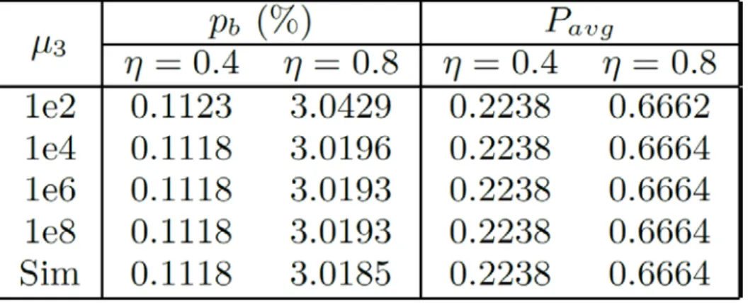
Example I – Case of Abondonments
•
𝐾𝐾
= 2
,
𝑇𝑇
(
1
)
= 10
,
𝑇𝑇
(
2
)
= 20
,
𝜇𝜇
1
= 0.5
,
𝜇𝜇
2
= 1
,
𝜂𝜂
=
𝜆𝜆
/
𝜇𝜇
2
•
Jobs with delays greater than
𝑇𝑇
(
2
)
= 20
abandon the system
•
𝑃𝑃
𝐼𝐼
= 0
,
𝑃𝑃
𝑘𝑘
=
𝜇𝜇
𝑘𝑘
2
•
Increase
𝜇𝜇
3
in order to model abandonments
Table 1: Blocking probability
𝑝𝑝
𝑏𝑏
and average system power
𝑃𝑃
𝑎𝑎𝑎𝑎𝑎𝑎
compared with
simulation results for two values of
𝜂𝜂
= 0.4, 0.8
.
Performance Modeling of Delay-based Dynamic Speed Scaling 25
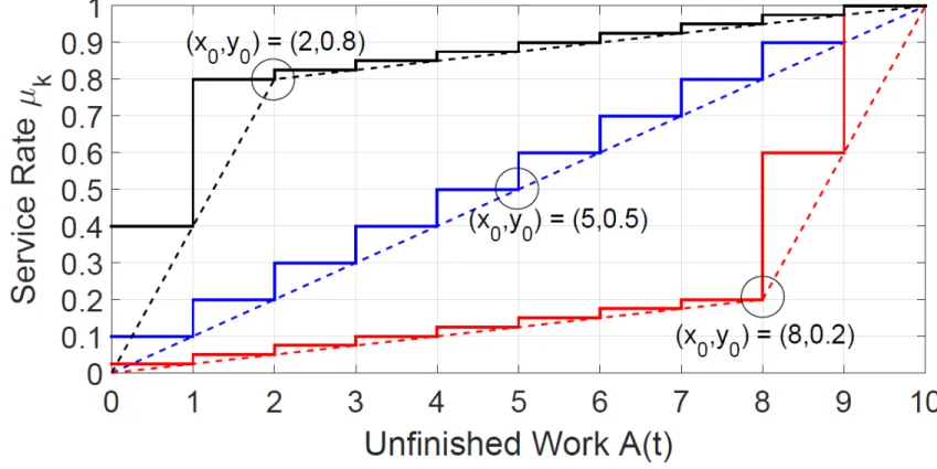
Example II – Piecewise Linear Rate
Adjustment Policy (PiLRAP)
•
Selects service rates from piecewise linear functions of the
unfinished work process
𝐴𝐴
(
𝑡𝑡
)
from the interval
𝜇𝜇
𝑚𝑚𝑖𝑖𝑚𝑚
,
𝜇𝜇
𝑚𝑚𝑎𝑎𝑑𝑑
.
•
𝜇𝜇
𝐾𝐾
=
𝜇𝜇
𝑚𝑚𝑎𝑎𝑑𝑑
•
Jobs with
𝐴𝐴 𝑡𝑡 ≥ 𝑇𝑇
(
𝐾𝐾
)
are blocked.
Performance Modeling of Delay-based Dynamic Speed Scaling 26
Example II – Piecewise Linear Rate
Adjustment Policy (PiLRAP)
Figure 1: Service rate function (dashed lines) and actual service rate
𝜇𝜇
𝐾𝐾
(straight lines)
as functions of
𝐴𝐴
(
𝑡𝑡
)
for
𝜇𝜇
𝑚𝑚𝑖𝑖𝑚𝑚
= 0
,
𝜇𝜇
𝑚𝑚𝑎𝑎𝑑𝑑
= 1
,
𝑇𝑇
(
𝐾𝐾
)
= 10
,
𝐾𝐾
= 10.
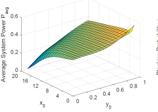
Performance Modeling of Delay-based Dynamic Speed Scaling 27
Figure 2: Average system power
𝑃𝑃
𝑎𝑎𝑎𝑎𝑎𝑎
and blocking probability
𝑝𝑝
𝑏𝑏
as functions of parameters
𝑥𝑥
0
and
𝑦𝑦
0
for
𝐾𝐾
= 20.
Example II – Piecewise Linear Rate
Performance Modeling of Delay-based Dynamic Speed Scaling 28
•
𝐾𝐾
= 1
,
𝑇𝑇
(
1
)
= 20
,
𝜇𝜇
1
=
𝜇𝜇
𝑚𝑚𝑎𝑎𝑑𝑑
= 1
•
M/M/1 queue with load
𝜌𝜌
=
𝜆𝜆
/
𝜇𝜇
𝑚𝑚𝑎𝑎𝑑𝑑
→ 𝑃𝑃
𝑓𝑓
= 1
− 𝜌𝜌 𝑃𝑃
𝐼𝐼
+
𝜌𝜌𝑃𝑃
1
•
𝐺𝐺
= 100
(
𝑃𝑃
𝑓𝑓
−𝑃𝑃
𝑎𝑎𝑎𝑎𝑎𝑎
)
𝑃𝑃
𝑓𝑓
•
Blocking probability should be less than 0.01
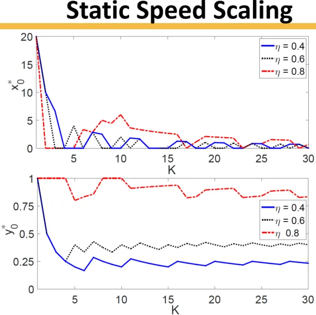
Example III – Comparison with
Performance Modeling of Delay-based Dynamic Speed Scaling 29
Figure 3: Optimal values of
𝑥𝑥
0
and
𝑦𝑦
0
, denoted by
𝑥𝑥
0
∗
and
𝑦𝑦
0
∗
, as functions of
𝐾𝐾
for
𝜂𝜂
= 0.4, 0.6, 0.8
.
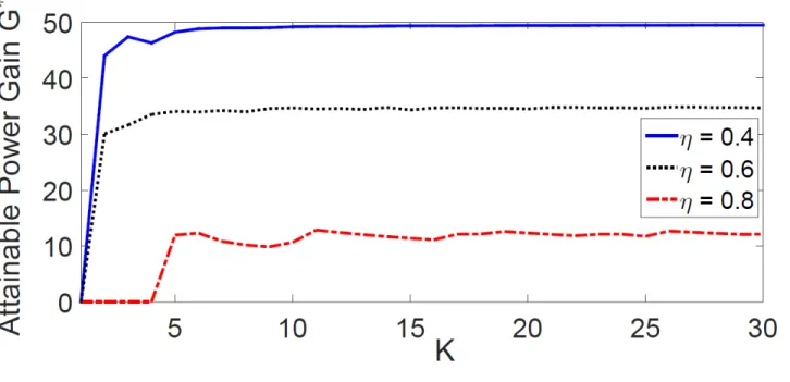
Example III – Comparison with
Performance Modeling of Delay-based Dynamic Speed Scaling 30
Figure 4: Attainable power gain, denoted by
𝐺𝐺
∗
, as a function of
𝐾𝐾
for
𝜂𝜂
= 0.4, 0.6, 0.8
.
Example III – Comparison with
Performance Modeling of Delay-based Dynamic Speed Scaling 31
Figure 5: Attainable power gain, denoted by
𝐺𝐺
∗
, as a function of the load
𝜂𝜂
for
𝐾𝐾
=20.
Example III – Comparison with
Performance Modeling of Delay-based Dynamic Speed Scaling 32
Conclusion
•
We propose an MRMFQ model of a dynamic speed
scaling system, in which a service rate is decided
according to the delay of the HOL job.
•
Piecewise Linear Rate Adjustment Policy (PiLRAP) is
proposed which minimizes the power consumption
under job blocking probability constraints.
Performance Modeling of Delay-based Dynamic Speed Scaling 33
Future Work
•
More general arrival process such as MAP
•
Other service time distributions, such Phase-type
distribution
•
Detailed analysis of a real life application
•
Zero-drift states to model abandonments to deal
with the case
𝜇𝜇
𝐾𝐾+1
→ ∞
Performance Modeling of Delay-based Dynamic Speed Scaling 34
Acknowledgment
•
This study is funded by
TÜBİTAK
(The Scientific and
Technological Research Council of Turkey) with ARDEB
1001 (under the project number 115E360) program.
Performance Modeling of Delay-based Dynamic Speed Scaling 36
Markov Fluid Queues (MFQs)
•
Single-Regime MFQ (SRMFQ)
Buffer considered as a single regime
Fixed infinitesimal generator and drift values
•
Multi-Regime MFQ (MRMFQ)
Buffer is divided into a finite number of regimes
Each regime has own infinitesimal generator and drift
values
•
Continuous-Feedback MFQ (CFMFQ)
Infinitesimal generator and drift values as continuous
Performance Modeling of Delay-based Dynamic Speed Scaling 37
𝐴𝐴
(
𝑘𝑘
)
=
𝑄𝑄
𝑘𝑘
𝑅𝑅
(
𝑘𝑘
)
−1
→
𝐴𝐴
(
𝑘𝑘
)
𝑌𝑌
(
𝑘𝑘
)
=
𝑌𝑌
(
𝑘𝑘
)
0
𝐴𝐴
−
(
𝑘𝑘
)
𝐴𝐴
(
+
𝑘𝑘
)
,
𝑌𝑌
(
𝑘𝑘
)
−1
=
𝐿𝐿
(
0
𝑘𝑘
)
𝐿𝐿
−
(
𝑘𝑘
)
𝐿𝐿
(
+
𝑘𝑘
)
→
𝑓𝑓
𝑘𝑘
𝑥𝑥
=
𝑑𝑑
𝑘𝑘
𝐿𝐿
(
0
𝑘𝑘
)
𝑒𝑒
𝐴𝐴
−
𝑘𝑘
(
𝑑𝑑−𝑇𝑇
(
𝑘𝑘−1
)
)
𝐿𝐿
−
(
𝑘𝑘
)
𝑒𝑒
−𝐴𝐴
+
𝑘𝑘
(
𝑇𝑇
𝑘𝑘
−𝑑𝑑
)
𝐿𝐿
(
+
𝑘𝑘
)
,
𝑑𝑑
𝑘𝑘
=
𝑑𝑑
0
(
𝑘𝑘
)
𝑑𝑑
−
(
𝑘𝑘
)
𝑑𝑑
+
(
𝑘𝑘
)
: vector of unknown coefficients
Performance Modeling of Delay-based Dynamic Speed Scaling 38
1.
Mean drift in the last regime should be negative, i.e.,
𝜋𝜋
(
𝐾𝐾
)
𝑅𝑅
(
𝐾𝐾
)
𝟏𝟏
< 0
2.
𝑓𝑓
𝐾𝐾
(
𝑥𝑥
)
should be bounded, i.e.,
𝑑𝑑
0
(
𝐾𝐾
)
= 0
,
𝑑𝑑
+
(
𝐾𝐾
)
=
𝟎𝟎
,
Performance Modeling of Delay-based Dynamic Speed Scaling 39