Volume 2009, Article ID 467549,10pages doi:10.1155/2009/467549
Research Article
Automatic Evaluation of Landmarks for
Image-Based Navigation Update
Stefan Lang and Michael Kirchhof
FGAN-FOM Research Institute for Optronics and Pattern Recognition, Gutleuthaußtr. 1, 76275 Ettlingen, Germany
Correspondence should be addressed to Michael Kirchhof,[email protected]
Received 29 July 2008; Revised 19 December 2008; Accepted 26 March 2009
Recommended by Fredrik Gustafsson
The successful mission of an autonomous airborne system like an unmanned aerial vehicle (UAV) strongly depends on its accurate navigation. While GPS is not always available and pose estimation based solely on Inertial Measurement Unit (IMU) drifts, image-based navigation may become a cheap and robust additional pose measurement device. For the actual navigation update a landmark-based approach is used. It is essential that the used landmarks are well chosen. Therefore we introduce an approach for evaluating landmarks in terms of the matching distance, which is the maximum misplacement in the position of the landmark that can be corrected. We validate the evaluations with our 3D reconstruction system working on data captured from a helicopter.
Copyright © 2009 S. Lang and M. Kirchhof. This is an open access article distributed under the Creative Commons Attribution License, which permits unrestricted use, distribution, and reproduction in any medium, provided the original work is properly cited.
1. Introduction
Autonomous navigation is of growing interest in science as well as in industry. The key problem of most existing outdoor systems is the dependency on GPS data. Since GPS is not always available we integrate an image-based approach into the system. Landmarks are used to update the actual position and orientation. Thus it is necessary to select the landmarks carefully. This selection takes place in an offline phase before the mission. The evaluation of these landmarks is the main contribution of this paper. For the online phase, we compute 3D reconstructions from the scene and match them with the selected georeferenced landmarks.
In our terms a landmark is a subset of a point cloud consisting of highly accurate LiDAR data.
There are already some systems that rely on image-based navigation by recognition of landmarks. At present all landmarks are manually selected by a human supervisor. We address the question if this is the optimal solution. The question arises since a human does the recognition or registration of the data due to very high level features while the system that has to deal with the landmarks operates on similarities on low level features such as the 3D point cloud.
The proposed automatic evaluation of landmarks in terms of matching distance (or convergence radius) enables
us to select the density of the landmarks in a manner that assures that even in the presence of IMU drift (which can be predicted from the previous measurements) the landmarks can still be recognized by the system.
The matching distance (or convergence radius), which is used in our evaluation method, is the maximum misplace-ment of the position of a landmark, that can be corrected. Thus it is a measure of the robustness of the considered landmark.
Scene reconstruction and (relative) pose estimation are very important tasks in photogrammetry and computer vision. Some typical solutions are given in [1–5]. While Akbarzadeh et al. [1] and Nist´er et al. [5] work with a camera system with at least two cameras with known relative position, they are able to determine the exact scale. In contrast the solutions in [2–4, 6] are only defined up to scale. In addition [6] evaluates the positioning problem in terms of occlusion, speed, and robustness. Our work is based on [7] where the 3D reconstrction is computed by feature tracking [8] and triangulation [9] from known camera positions.
Online phase Offline phase
Evaluation of landmarks
Fusion and path planning
Structure from motion
Image based navigation update
Landm ar
k
Final landm
ark position
Figure 1: Overview of our landmark-based navigation system. In the offline phase before the mission landmarks are evaluated and fused with the path planning. During the online phase the navigation data are updated by mean of the registation of the landmarks with the SfM point cloud.
Navigation System (INS) or in absence of GPS of the IMU alone—resulting in fewer parameters in the registration process, which is based on Iterative Closest Point (ICP) [10] in our approach. Reference [11] showed an application of ICP-based registration of continuous video onto 3D point clouds for optimizing the texture of the point cloud. A different solution to the registration that is not adressed here is described in [6]. Lerner et al. [12] provide a solution to pose and motion estimation based on registration with a Digital Terain Model (DTM). While saving the DTM for the complete flight path is critical we focus on the selection of “good” landmarks. For pedestrians and cars some evaluations of landmarks had been done in terms of permanence, uniqueness, and visibility [13–17]. In our context uniqueness and matching distance are the most relevant factors.
Our paper is organized as follows. The second part of the paper describes the different methodologies used throughout the paper. The focus is on the evaluation of landmarks, which is described first. Path planning by means of given landmarks, a simple approach for 3D-reconstruction and an approach to image-based navigation update are outlined as part of the complete system. In the following part experiments, first the experimental setup and used data sets are presented. Then we give the results of the evaluation of several landmarks. Additionally results of tests of the complete system are shown. The paper closes with a discussion and conclusion.
2. Methodology
It is assumed that highly accurate 3D data of an area are given. A landmark will be called optimalif the probability to recover it in the later mission is maximal. For that purpose
meaningful measures for evaluation of landmarks have to be developed.
In contrast to simply defining a cost function for evaluation of a landmark, the method to find the landmark is used directly for evaluation. As further requirement the rotation and translation which align the reconstructed area with the found landmark are needed. For that purpose the ICP method [10] is used, which is a standard approach for registering two point clouds.
The evaluation and thus the selection of landmarks will take place in an offline phase before the mission. In this phase all given information are fused and the path planned. Then during mission in the online phase, both the reconstructed point cloud, obtained by the SfM system, and the landmarks are registered and the final landmark position estimated. The calculated transformation information can be used for an image-based navigation update. The whole system is presented inFigure 1.
2.1. Evaluation of Landmarks. A landmark given by many highly accurate 3D points will be evaluated by means of all available information. Considering the functionality of the used ICP, the following design issues are important.
(i) Size and structure of the landmark.
(ii) Structure of the local area surrounding the landmark. (iii) Uniqueness of the landmark in the wider considered
area.
These issues led to a combination of a local and a global evaluations. The local evaluation fulfills the constraints in taking the size and structure of the landmark as well as the structure of the surrounding area into account. A house in a highly cluttered area is not a very meaningful landmark since ICP would not be able to retrieve the exact orientation of the landmark and thus should get a bad evaluation. The third constrain, the uniqueness of the landmark in the considered area, needs a global view on the area. Objects similar to the tested landmark, which could lead to confusion in the recovery process have to be detected and therefore should receive a bad evaluation result. For example a house next to a similar house is not a very meaningful landmark and thus should get a bad evaluation.
2.1.1. Local Evaluation. LetDlandmark be a set of 3D points describing a landmark and letDarea be a set of 3D points defining the given area. If there is an error in the estimated pose of the observer, the area will be rotated and translated. Thus the coordinate system is first rotated around the center of the landmark withRand then shifted byt. The rotation matrixRis constructed as follows:
R= ⎛ ⎜ ⎜ ⎝
cos(θz) −sin(θz) 0
sin(θz) cos(θz) 0
0 0 1
⎞ ⎟ ⎟
⎠, (1)
whereθzis the rotation angle around thez-axis. The changes in the 3D pointsp∈R3ofD
areacan be calculated with
Darea =
Input parameters:Dlandmark,Darea,dx,dy,θmax
1:for all−θmax≤θz≤θmaxdo
2: for all−dy≤y≤dydo 3: for all−dx≤x≤dxdo 4: t←(x,y, 0)T 5: R←euler2rot(θz)
6: Darea← {p|p=Rp+t,p∈Darea} 7: Rcalc,tcalc←ICP(Darea,Dlandmark)
8: t(x,y)← t−tcalc
9: θ(x,y)← |θz−rot2eulerz(Rcalc)|
10: end for
11: end for
12:end for
Algorithm1: Landmark grid test method.
For the evaluation a landmark is tested for different translations and rotations. As already mentioned in (1) we ignore rotations and translations that effect the ground plane (z = 0) for reducing the complexity of the simulation. The previous experiments showed that these parameters can be ignored because ICP always registered the ground plane correct, because all the data expand along this plane.
In each cycle the ICP algorithm is performed withDarea andDlandmark. For later evaluation the position errort(x,y) and rotation error θ(x,y) in a grid around the landmark position and different angles are calculated. Algorithm 1
shows the implementation of this “Landmark Grid Test Method.” The algorithm iterates over all angles and grid points given by the input parameters. The used methods
euler2rotandrot2eulerconvert a rotation angle to a rotation matrix and vice versa. As main function call, see step 7, the method ICP calculates the transformation parameters aligningDarea withDlandmark.
For each applied angle θz ∈ [−θmax,θmax] the error images t andθ are obtained. These slices contain errors with respect to translation and rotation for each grid point. They are converted by means of defined thresholds for maximum allowed translation and rotation error. The results are binary images with the entry one where the method converged to the right result and zero otherwise. The sum of all ones in each slice is used as a measure for the evaluation and comparison of the landmarks. Additionally vectors to the minimum and maximum grid points with a value one are used in the evaluation of the landmarks, too. These vectors are depicted in the second row of Figure 9. Appart from the evaluation measure they define a minimal and maximal matching distance which is required for the path planning. While the minimal matching distance is equivalent to the radius of convergence, the maximum matching distance is the largest distance from which the ICP converged against the solution.
2.1.2. Global Evaluation. In global consideration a landmark will be evaluated by means of the whole area. For that purpose a binary mask of the area is generated, by projecting the 3D points to an image plane parallel to (z = 0) with a
pixel size of 10 by 10 meters. The entries of this image are one if there is at least one 3D points projected to the pixel otherwise zero. Next, the binary image is preprocessed for our purposes by means of morphological operations. First the operation closing is performed to fill holes (zeros) in the mask of the area. Then the mask is eroded with a mask of the landmark as structured element to avoid the border of the area. The different steps of this approach are shown in
Figure 2.
For each entry of the mask equal one, the landmark is moved to the corresponding position in the area but not rotated and the ICP method is applied. The result is assigned to that position. With this described approach local minima with respect to the ICP’s cost function can be spotted. The global minimum is expected to be at the center of the origin landmark position.
Considering that the ICP error functionerficp is a sum of least squares, the error function is equivalent to the Log-Likelihood function describing the probability that the data are an instance of the model. The original likelihood is a natural measure for the instances. Assuming that ICP converges towards the global minimum Xglobalmin (ground truth) or the second smallest local minimum Xlocalmin the probability for matching the model with the ground truth is given by
G= e−erficp(Xglobalmin)
e−erficp(Xglobalmin)+e−erficp(Xlocalmin). (3)
Indeed this measure depends on the precision of the data. But assuming that all the derived 3D points have approximately the same deviation (approximately one) there is just a linear scaling between the likelihood and the probability which is approximately compensated by the denominator in (3). The normalization leads to the codomain [0, 1).
2.2. Fusion and Path Planning. When selecting landmarks for navigation the first problem one has to address is the uniqueness of the landmarks. A measure for the uniqueness is the discriminatory power of the landmarks to local minima during the ICP/registration process. In the absence of the absolute probabilities, randomly chosen landmarks within a search region are first sorted by the global measure (3) which corresponds to the discriminatory power. The best 20% of the landmarks are treated further with the local evaluation.
The local evaluation gives a measure for the volume of the parameter space from which ICP converges against the ground truth. Therefore it is related to the speed of convergence and the radius of convergence. Within the local evaluation one can compute the smallest distance of the surface to the reference position. This distance describes the precision that the UAV should have during approaching the landmark. Knowing the drift of the UAV one can define the search region for the next landmark.
(a) (b) (c)
Figure2: Creation of the binary mask for the tests. (a) Initialized mask with black pixels if a 3D laser point is found in the defined neighborhood. (b) Mask after the closing operation. (c) The gray area is eroded by means of a mask of the landmark as structured element (upper left, red box). The final mask consists of the residual black pixels.
or randomly chosen landmarks. These landmarks are then evaluated with the methods described in Sections2.1.1and
2.1.2 resulting in a decision for the best landmark. This method is repeated until one reaches the starting point of the UAV.
2.3. Structure from Motion/3D Reconstruction. In this section the Structure from Motion (SfM) system to calculate a 3D point cloud from given IR images is described briefly. Additionally the approach using orientation and position information of the sensor to obtain more accuracy in the reconstruction is described. The implementation is based on Intel’s computer vision library OpenCV [18].
A system overview is given inFigure 3. After initializa-tion, detected features are tracked image by image. In order to minimize the number of mismatches between the corre-sponding features in two consecutive images the algorithm checks the epipolar constraint by means of the given pose information retrieved from the INS. Triangulation of the tracked features results in the 3D points. Each 3D point is assessed with the aid of its covariance matrix which is associated with the respective uncertainty. Finally a nonlinear optimization yields the completed point cloud.
The modules are described in more detail in the following sections.
2.3.1. Tracking Features. To estimate the motion between two consecutive images the OpenCV version [19] of the KLT tracker [8] is used. The algorithm tracks corners or corner-like point features. For robust tracking a measure of feature similarity is used. This weighted correlation function quantifies the change of a tracked feature between the current image and the image of initialization of the feature.
2.3.2. Retrieve Orientation and Position. The INS gives the Kalman-filtered [20] absolute position and orientation of the reference coordinate frame. After converting the data into absolute rotation matrices Rabsi and position vectorsCi for the absolute orientation and position of theith camera in space, the projection matrices Pi, needed for triangulation, are calculated as follows:
Pi=KRabsi
I3| −Ci
, (4)
where K is the intrinsic camera matrix and Pia 3×4-matrix.
IR-images
Track features
Check features
Triangulate
Refine 3D points
3D point cloud IMU/GPS
Pose/position Retrieve pose and position
Figure3: Overview of the SfM modules. Features are tracked in consecutive images and checked for satisfaction of the epipolar constraint. Linear Triangulation of each track of the checked features gives the 3D information. In both steps—constraint checking and triangulation—the retrieved orientation and position information is used. Finally each 3D point are evaluated and optimized.
2.3.3. Epipolar Constraint. With the aid of the epipolar con-straint mismatches in the feature tracking can be detected. Both the relative rotation R and the relative translation t between two consecutive images are given. As described in [3] the fundamental matrix can be calculated according to
F=KT−1[t]×RK−1. (5)
With the skew-symmetric matrix [t]× of the vector t. To check whetherx is the correct image point corresponding to the tracked point featurexof the previous image,xhas to lie on the epipolar lineldefined as
distance (error) ofx tol. But we reject the feature if the distance becomes too large and the track ends.
2.3.4. Triangulation. During iteration over the IR images, tracks of detected and tracked point features are built and the corresponding 3D point Xis calculated. In [9] a good overview of different methods for triangulation is given as well as a description of the method used in our system.
Letx1,. . .,xn be the image features of the tracked 3D
pointX innimages and P1,. . ., Pnthe projection matrices of the corresponding cameras. Each measurementxi of the track represents the reprojection of the same 3D point
xi≡PiX fori=1,. . .,n. (7)
With the cross-product the homogeneous scale factor of (7) is eliminated, which leads toxi×(PiX)= 0. Subsequently there are two linearly independent equations for each image point. These equations are linear in the components of X, thus they can be written in the form AX=0, where A is the corresponding action matrix [9]. The 3D pointXis the unit singular vector corresponding to the smallest singular value of the matrix A.
2.3.5. Nonlinear Optimization. After triangulation the repro-jection error can be estimated as follows:
i=
⎛ ⎝
x i
iy ⎞
⎠=d(X, Pi,xi)= ⎛ ⎜ ⎜ ⎜ ⎜ ⎝
xi− p1
iX p3
iX
yi− p2
iX p3iX ⎞ ⎟ ⎟ ⎟ ⎟
⎠. (8)
With the assumption of a variance of the 2D position of one pixel, the back-propagated covariance matrix of a 3D point is calculated
ΣX=
JTΣ−1
p J
−1
. (9)
In this case the covariance of 2D position Σ−1
p equals the 2D identity matrix, with the Jacobian matrix J, which is the partial derivative matrix∂/∂X. The Euclidean norm ofΣX gives an overall measure of the uncertainty of the 3D pointX and enables the algorithm to reject poor triangulation results. With nonlinear optimization, a calculated 3D point can be corrected. Using the Gauss-Newton method [21] yields the corrected 3D points.
2.3.6. Results. Working on an IR sequence with 470 images and taking orientation and position information into account the system had calculated an optimized point cloud of about 17 500 points seeFigure 4. The height of each point is coded in its color. Although it is a sparse reconstruction, the structure of each building is well distinguishable and there are only a few gross errors due to the performed optimization.
2.4. Image-Based Navigation Update in the Complete System.
In the previous sections only highly accurate 3D points are
Figure 4: Calculated point cloud of an IR image sequence with the magnification of one building. The overall number of points is 17 606.
used for evaluation or selection of landmarks. That can be considered as the preparation phase of a mission, where LiDAR or other advanced sensors are used for measuring the structure of the area.
The goal of the image-based navigation update is to correct the INS drift with the help of the selected landmarks. For this purpose the system descriped inSection 2.3is used to estimate a 3D point cloud on base of the INS poses during the flight. Aligning this point cloud with the accurate landmark models yields the transformation that is needed to correct for the INS drift.
3. Experiments
3.1. Experimental Setup. As sensor platform a helicopter is used. The different sensors are installed in a pivot-mounted sensor carrier on the right side of the helicopter. The following sensors are used.
IR camera. An AIM 640QMW is used to acquire midwave-length (3–5μm) infrared light. The lens has a focal length of 28 mm and a field of view of 30.7◦×23.5◦. LiDAR. The Riegl Laser Q560 is a 2D scanning device which
illuminates in azimuth and elevation with short laser pulses. The distance is calculated based on the time of flight of a pulse. It covers almost the same field of view as the IR camera.
INS. The Inertial Navigation System (INS) is an Applanix POS AV system which is specially designed for air-borne usage. It consists of an IMU and a GPS system. The measured orientation and position are Kalman-filtered to smooth out errors in the GPS.
Figure5: Oblique view of the considered LiDAR area.
I
IV III
II
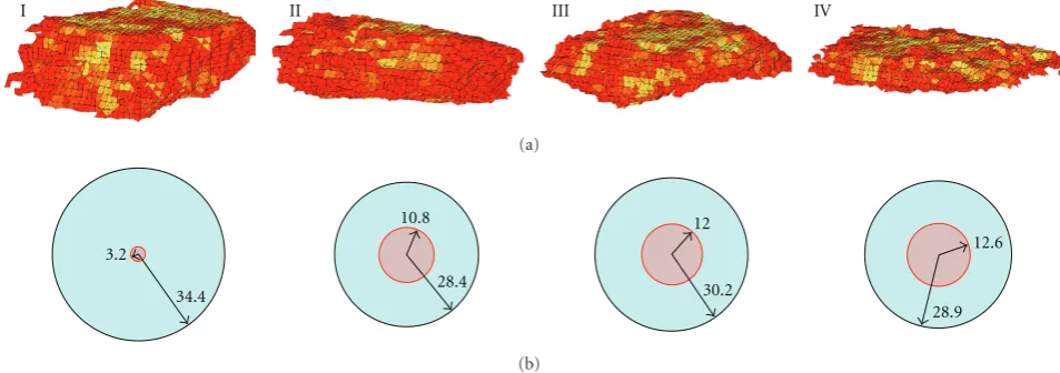
Figure 6: The four manually chosen landmarks (I–IV). Each landmark is of different size and structure.
Both the coordinate frame of the IR camera and of the laser scanner are given with respect to the INS reference coordinate frame. Therefore coordinate transformations between the IR camera and the laser scanner are known.
3.2. Used Data Sets. For evaluation of the landmarks, LiDAR data are used. The point cloud consists of highly accurate 3D points. The results should be meaningful regarding the later usage in a system working with 3D points calculated by Structure from Motion algorithms as described in Section 2.3. For that purpose the LiDAR point cloud is randomly downsampled by factor 100 for the evaluation. However the evaluated landmarks are only randomly downsampled by factor 10. These landmarks will be used in the later navigation update process which runs in real time.
The LiDAR point cloud of the considered area is presented inFigure 5.
For tests two different types of landmarks are used. The main difference between these manually and randomly chosen landmarks is the criteria applied by the selection. The manually selected landmarks normally contain whole buildings and other obvious structures; whereas the other selection strategy works completely random.Figure 6shows the manually chosen landmarks. Each landmark is of different size and structure. The first one is a single building, whereas the second landmark consists of that building and parts of neighboring buildings. In the third landmark there are also trees and a few building parts. A long strip over almost the whole considered area is used as fourth landmark. Additionally to these four manually chosen landmarks, three landmarks are selected randomly. The selection of these
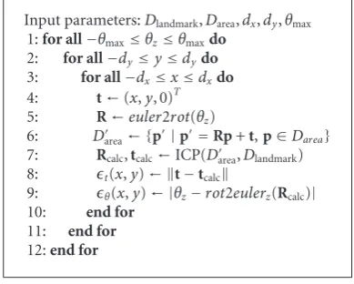
AI AII
AIII
Figure7: The three randomly chosen landmarks (AI–AIII).
landmarks is not oriented on buildings or structure (see
Figure 7).
3.3. Evaluation of Landmarks. As described inSection 2.1.1
each landmark is locally evaluated by means of a grid search for the size of its region of convergence. Images of the absolute position and rotational errors for the four manually selected landmarks are shown inFigure 8. For each landmark (I–IV) are two rows of error images presented. The first row consists of images of the angular errorsθ. In the second row the translation errorstare shown. Each column represents a different tested rotation of the landmark from−12 degree to +12 degree. The size of the test grid is 61×61 meters, thus 30 meters in each direction. Because of that, the resolution of the error images is 61×61. Darker means less error. Each type of error is scaled uniformly through the four landmarks. Only small errors are accepted as correct result, thus thresholds for θ and t are defined as three degrees and two meters. The obtained binary imagesθ andt are simply linked through
total=θ ∧t. (10)
Stacking these combined binary images for all different rotations, volumes of convergence are obtained. This graphic rendition gives a good overview of the different behavior of the ICP method for the landmarks. The volumes are illustrated in the first row of Figure 9. We take the sum of all binary volume slices as local evaluation measure for comparison. The radii of convergence are shown in the second row of the figure. For each landmark the minimum and maximum vectors are plotted, where the right position and rotation could be retrieved. Additionally a red and a blue circles symbolize the radius of convergence.
I
II
III
IV θ
t
θ
t
θ
t
θ
t
−12◦ −8◦ −4◦ 0◦ 4◦ 8◦ 12◦
Figure8: Results of local evaluation for the four landmarks. For each landmark (I–IV) the error imagesθandtare shown for different rotation. All images of the same error type are scaled in the same way. Darker means less error.
The dimensions of the bounding boxes, and the number of laser points reveals the sizes of the landmarks. The local evaluation (volume) and the global evaluation measures are displayed to compare the landmarks.
3.4. Tests in the Complete System. Until now all tests were performed only with highly accurate LiDAR data. In this section we present the performance evaluation of the landmarks aligned with the reconstructed point cloud from the IR sequence (see Figure 4) via ICP. For the tests the same method as for the local evaluation is used. However, in contrast to the evaluation we have chosen a different grid for the search. As before 30 meters in every direction was searched, but the distance between the grid points was increased two meters instead of one meter because the details of the areas do not matter. Since the drift of the IMU
in the rotation is very small due to single integration of the measurement instead of double integration as for the translation, we restricted the rotations to a maximum three degrees in the tests.
Figure 10 shows the results of the test runs. The error images θ andt for the four landmarks are of the same scale as inFigure 8. Additionally the radii of convergence are shown on the right side of the figure.
4. Discussion
I II III IV
(a)
34.4 3.2
10.8
28.4
12
30.2
12.6
28.9
(b)
Figure9: (a) The evaluated volume of landmarks I to IV. Note that the volumes are scaled to match the image domain. (b) The radii of convergence of the landmarks. The red circle and the corresponding vector are the minimum area, where the method converges to the right result. The maximum distance is displayed by the blue circle with its maximum vector.
Table1: Overview of the evaluation results of the manually and randomly selected landmarks.
Manually Randomly
I II III IV AI AII AIII
Bounding Box [m] 98×93 204×147 182×151 636×67 145×60 145×115 230×145
Number of points 28265 80764 42135 82142 4374 35998 96823
Local evaluation (volume) 4470 4578 5679 3942 2084 6009 6134
Global evaluation equation (3) 0.5063 0.7458 0.7279 0.7410 0.5065 0.6495 0.7215
than smaller landmarks. Smallest errors, which means the biggest dark area, is found in the fourth column, with no rotation applied, as expected.
A better overview of the total volume of convergence is given byFigure 9, first row. The volume of convergence is the integration of all possible misplacements and rotations of the tested landmark from, where the ICP algorithm converges. Because of the different scale the size of the volumes cannot be compared by observation. Well distinguishable are the shapes of the volumes. Each landmark has its characteristic shape of the volume of convergence. Nevertheless for the navigation approach only the minimal matching distance matters. In the second row, the radii of convergence of the landmarks are illustrated. The maximum radius of landmark I is better than those of the others; however it lacks in the minimum convergence radius. That means that if the landmark is seen from the wrong direction, just a small misplacement can lead to a wrong result. In that manner the other bigger landmarks are more robust.
Manually and randomly chosen landmarks are compared with each other in Table 1. The results are summarized quantitatively. The smaller landmarks I and AI got a bad local and global evaluation result. The best local evaluation was obtained by landmark A3, which is also the biggest landmark. Although in the global evaluation landmark II got the best result. The long strip, landmark IV, performs quite well in the global consideration whereas it lacks of local robustness.
The other landmarks in the midfield are all comparable. As result we conclude that size does matter but not as significant as expected. Landmarks greater than certain sizes perform well, and there is no evidence that smaller landmarks are not as reliable as larger ones. The randomly selected landmarks scored a little higher in the local evaluation but apart from that there is no significant difference between the manually and randomly selected landmarks. We suggest that using the automatic selection method desrcibed in Section 2.2 with a large number of randomly generated landmarks would result in comparable or even better results than using manual selected landmarks.
Focusing on the results of the tests with the SfM point cloud (seeFigure 10), the following issues are significant.
(i) The error images of the local evaluation (seeFigure 8) of LIDAR data and those of the SfM test (see
Figure 10) are striking similar.
(ii) The radii of convergence and the corresponding vectors for both the local evaluation and the results with the calculated point cloud are also similar with a few exceptions.
7.2
27.2
11.6
28.4
2
20 0
39.6 I
SfM
II SfM
III SfM
IV SfM
θ
t
θ
t
θ
t
θ
t
−3◦ 0◦ +3◦
Figure10: Results of tests with the calculated SfM point cloud. As described inFigure 8for each landmark the error images are given. Additionally the radii of convergence are shown for each landmark on the right side.
5. Conclusion
For navigation update a landmark-based approach using the ICP method is suggested. The success of the used ICP method for registering two point clouds (a model of the landmark and the area) is very dependent on the size and structure of the landmark model. Using such an approach for a navigation update therefore strongly depends on the chosen landmarks. Thus it is important to select the landmarks very carefully. Additionally the result of this approach is normally not unique on a considered area, therefore local minima may occur.
We introduced a landmark evaluation which consists of both local and global considerations reflecting uniqueness and matching distance. For evaluation the same method is used as in the later registering process. Tests with real IR images and calculated 3D points showed that this evaluation measure is transferable to the detection performance in the
later application in the proposed system for image-based navigation update.
This transferability is caused by using the same registra-tion method for evaluaregistra-tion of the landmarks and navigaregistra-tion. The concept can be transferred to any registration method giving a measure for the matching quality.
Acknowledgments
The authors like to thank Professor Maurus Tacke, Dr. Karl L¨utjen, and Klaus J¨ager for the support and creating a good environment for our research. For the many discussions and remarks the authors thank Dr. Michael Arens and Dr. Rolf Sch¨afer. Last but not least, the authors thank Marcus Hebel for processing the LiDAR data.
References
[1] A. Akbarzadeh, J.-M. Frahm, P. Mordohai, et al., “Towards urban 3D reconstruction from video,” inProceedings of the 3rd International Symposium on 3D Data Processing, Visualization, and Transmission (3DPVT ’06), pp. 1–8, Chapel Hill, NC, USA, June 2006.
[2] A. J. Davison, I. D. Reid, N. D. Molton, and O. Stasse, “MonoSLAM: real-time single camera SLAM,”IEEE Transac-tions on Pattern Analysis and Machine Intelligence, vol. 29, no. 6, pp. 1052–1067, 2007.
[3] R. I. Hartley and A. Zisserman,Multiple View Geometry in Computer Vision, Cambridge University Press, Cambridge, UK, 2nd edition, 2004.
[4] D. Nist´er, Automatic dense reconstruction from uncalibrated video sequences, Ph.D. dissertation, Royal Institute of Technol-ogy, Stockholm, Sweden, March 2001.
[5] D. Nist´er, O. Naroditsky, and J. Bergen, “Visual odometry for ground vehicle applications,”Journal of Field Robotics, vol. 23, no. 1, pp. 3–20, 2006.
[6] M. Rodrigues, R. Fisher, and Y. Liu, “Special issue on registration and fusion of range images,”Computer Vision and Image Understanding, vol. 87, no. 1–3, pp. 1–7, 2002. [7] S. Lang, M. Hebel, and M. Kirchhof, “The accuracy of scene
reconstruction from IR images based on known camera positions—an evaluation with the aid of lidar data,” in
Proceedings of the 3rd International Conference on Computer Vision Theory and Applications (VISAPP ’08), vol. 2, pp. 439– 446, Funchal, Portugal, January 2008.
[8] J. Shi and C. Tomasi, “Good features to track,” inProceedings of IEEE Computer Society Conference on Computer Vision and Pattern Recognition (CVPR ’94), pp. 593–600, Seattle, Wash, USA, June 1994.
[9] R. I. Hartley and P. Sturm, “Triangulation,”Computer Vision and Image Understanding, vol. 68, no. 2, pp. 146–157, 1997. [10] P. J. Besl and N. D. McKay, “A method for registration of
3-D shapes,”IEEE Transactions on Pattern Analysis and Machine Intelligence, vol. 14, no. 2, pp. 239–256, 1992.
[11] W. Zhao, D. Nist´er, and S. Hsu, “Alignment of continuous video onto 3D point clouds,” IEEE Transactions on Pattern Analysis and Machine Intelligence, vol. 27, no. 8, pp. 1305– 1318, 2005.
[12] R. Lerner, E. Rivlin, and H. P. Rotstein, “Pose and motion recovery from feature correspondences and a digital terrain map,” IEEE Transactions on Pattern Analysis and Machine Intelligence, vol. 28, no. 9, pp. 1404–1417, 2006.
[13] C. Brenner and B. Elias, “Extracting landmarks for car naviga-tion systems using existing gis databases an+d laser scanning,” inProceedings of International Archives of the Photogrammetry, Remote Sensing and Spatial Information Sciences (ISPRS ’03), pp. 131–136, Munich, Germany, September 2003.
[14] G. Burnett, D. Smith, and A. May, “Supporting the navigation task: characteristics of good landmarks,” inProceedings of the
Annual Conference of the Ergonomics Society, pp. 441–446, Turin, Italy, November 2001.
[15] G. Burnett,Turn right at the kings head drivers requirements for route guidance information, Ph.D. dissertation, Loughorough University, Leicestershire, UK, 1998.
[16] K. L. Lovelace, M. Hegarty, and D. R. Montello, “Ele-ments of good route directions in familiar and unfamiliar environments,” inSpatial Information Theory: Cognitive and Computational Foundations of Geographic Information Science, vol. 1661 ofLecture Notes in Computer Science, pp. 65–82, Springer, New York, NY, USA, 1999.
[17] P.-E. Michon and M. Denis, “When and why are visual landmarks used in giving directions?” inProceedings of the International Conference on Spatial Information Theory, vol. 2205 of Lecture Notes in Computer Science, pp. 292–305, Springer, Morro Bay, Calif, USA, September 2001.
[18] Intel, “Opencv—open source computer vision library,” 2006,
http://www.intel.com/technology/computing/opencv. [19] J.-Y. Bouguet, “Pyramidal implementation of the lucas kanade
feature tracker,” Tech. Rep. OpenCV documentation, Micro-processor Research Labs, Intel Corp., Santa Clara, Calif, USA, 2000.
[20] G. Welch and G. Bishop, “An introduction to the Kalman filter,” Tech. Rep. 95-041, Department of Computer Science, University of North Carolina at Chapel Hill, Chapel Hill, NC, USA, May 2003.