Schedule Analysis Using Earned Value Concepts ABSTRACT

(1)

G.R. Cathcart & Erica Smith Tecolote Research, Inc.

ABSTRACT

Tecolote has developed a procedure to compare two schedules to determine if activities are ahead of or behind schedule. For on-going activities, we calculate the rate of progress of each activity based on the time since the start date and the reported "percent complete," then apply that rate to find a corrected finish date for the activity. If an activity's corrected finish date exceeds the slack available for the activity, it is flagged for management attention (a negative number in the Total Slack column below).

NAME DUR START FINISH

% Complete Total Slack Projected % Complete Status BL % Complete Projected BL Status Projected Completion Date Change in Finish Date Total Slack - Change Finish Date

Activity 1 527 10/9/01 11/18/03 55% 21 86% Behind 100% Behind 6/28/04 159 -138

Activity 2 327 6/24/02 10/10/03 67% 48 85% Behind 100% Behind 12/29/03 56 -8

Activity 3 0 11/18/03 11/18/03 0% 21 0% Not Sked 100% Behind 11/18/03 0

Activity 5 120 1/24/05 7/5/05 0% 208 0% Not Sked 0% Not Sked 7/5/05 0

Activity 6 431 11/25/02 8/19/04 86% 400 39% Ahead 100% Behind 10/23/03 -217 617

Activity 7 319 7/1/02 10/7/03 88% 654 86% On Sked 100% Behind 10/7/03 0

Activity 8 522 10/1/01 11/3/03 80% 635 88% Behind 100% Behind 12/24/03 37 598

Activity 9 354 4/8/02 9/4/03 85% 677 93% Behind 42% Ahead 10/14/03 28 649

Activity 10 333 3/1/01 6/28/02 100% 0 100% Complete 100% Complete 6/28/02 0

We have also developed a process of converting the schedule data into the same type of data that is used in the Earned Value process, except instead of using dollars from the budget to determine the Schedule Variance (SV) and Schedule Performance Index (SPI), we use time in the form of the schedule. We then compare to two processes to determine if the trends are conveying the same information. NAME DUR % Complete Proj % Complete Status Estimate Duration at Completion (EDAC) Schedule B Actual Work Performed (AWP) Schedule B Planned Duration At Completion (PDAC) Schedule B Estimate Duration To Completion (EDTC) Schedule B Planned Work Scheduled (PWS) Schedule B BL Work Planned (BWP) Schedule B Schedule Variance (SV) Schedule B Schedule Index (SI) Schedule B Variance At Completion (DVAC) Schedule B Activity 1 527 55% 86% Behind 709 290 527 237 452 183 -163 0.64 -182.00 Activity 2 327 67% 85% Behind 395 219 327 107 278 49 -59 0.79 -68.00

Activity 3 0 0% 0% Not Sked 0 0 0 0 0 0 0 0.00 0.00

Activity 4 299 33% 93% Behind 488 99 299 200 277 49 -178 0.36 -189.00

Activity 6 431 86% 39% Ahead 238 371 431 60 170 109 201 2.18 193.00 Activity 7 319 88% 86% On Sked 331 281 319 48 273 213 8 1.03 -12.00 Activity 8 522 80% 88% Behind 582 418 522 104 458 408 -40 0.91 -60.00 Activity 9 354 85% 93% Behind 396 301 354 53 330 344 -29 0.91 -42.00 Activity 10 333 100% 100% Complete 333 333 333 0 333 333 0 1.00 0.00 NAME DUR % Complete Proj % Complete Status Estimate Duration at Completion (EDAC) Schedule B Actual Work Performed (AWP) Schedule B Planned Duration At Completion (PDAC) Schedule B Estimate Duration To Completion (EDTC) Schedule B Planned Work Scheduled (PWS) Schedule B BL Work Planned (BWP) Schedule B Schedule Variance (SV) Schedule B Schedule Index (SI) Schedule B Variance At Completion (DVAC) Schedule B Activity 1 527 55% 86% Behind 709 290 527 237 452 183 -163 0.64 -182.00 Activity 2 327 67% 85% Behind 395 219 327 107 278 49 -59 0.79 -68.00

Activity 4 299 33% 93% Behind 488 99 299 200 277 49 -178 0.36 -189.00

Activity 6 431 86% 39% Ahead 238 371 431 60 170 109 201 2.18 193.00 Activity 7 319 88% 86% On Sked 331 281 319 48 273 213 8 1.03 -12.00 Activity 8 522 80% 88% Behind 582 418 522 104 458 408 -40 0.91 -60.00 Activity 9 354 85% 93% Behind 396 301 354 53 330 344 -29 0.91 -42.00 Activity 10 333 100% 100% Complete 333 333 333 0 333 333 0 1.00 0.00

(2)

INTRODUCTION

Schedule analysis is a discipline that enables a program’s management team to assess the health and progress of the project. Specifically, schedule analysis provides insight into viability of and the progress toward accomplishing the program plan. While the analysis may reveal activities that are ahead of schedule as well as behind, the primary concern is identifying activities that are behind schedule and trying to determine the impact on the estimated project finish date. When activities are identified as being behind, the analyst is able help the management team define their priorities in terms of resources and attention. With a well-developed schedule, an analyst is able to provide a quality independent estimate at completion for key activities and the entire project. The analysis results aides the project team in developing and evaluating proposed changes to the project plan.

This paper demonstrates a straightforward methodology for analyzing schedules using both the typical type of analysis and the generally accepted and familiar concepts of Earned Value Management (EVM). A well-developed, and well-maintained network schedule can be used to provide great insight into the overall performance of a program. We generally think of the results of schedule analysis in terms of critical path, slack, and completion date. Provided that the schedule network is properly built and maintained, this paper will demonstrate that we can also present the schedule status as it varies from the baseline schedule. Empirically, we have discovered that variances in the analysis of schedule data lead variances in the analysis of EVM data by one month

This paper is organized into three sections. The first discusses Schedule Quality, specifically how a schedule network is developed and how a schedule status review is performed. The second section covers certain Key Schedule Metrics that the program management team may use to formulate a quick assessment of the project and the schedule’s quality. The last section describes how an analyst may incorporate traditional Earned Value concepts into schedule analysis.

SCHEDULE QUALITY

A schedule should reflect the program plan and provide insight into whether the program can be executed successfully. A quality schedule is important primarily because a poorly built one, which is often just a Gantt chart, can mask significant program problems. A quality schedule is constructed using a number of common sense guidelines. They include:

• link activities, i.e., they have predecessors and successors as appropriate

• do not link summary tasks

• minimize the number of milestone activities

• ensure that activity durations reflect planned work and work packages.

• avoid using these limiting constraints:

o Must Finish On

o Must Start On

o Finish No Later Than

(3)

During the development of a network schedule, it is critical that the schedule analyst follows the schedule development guidelines. It is also advisable that the network schedule be reviewed and evaluated periodically to ensure that these guidelines are being followed.

There are several warning flags will indicate the overall quality of the schedule. These signs include:

• Unlinked activities

• Summary tasks with links

• Excessive summary and milestone activities

• Misused and overused constraints

Unlinked Activities.

The first warning flag is a significant number of activities or milestones without predecessors or successors (links). Activities without predecessors are usually the first activity in a chain. When this is due to a number of different chains starting at the same time, often near the project start, but not connected to a starting activity, there is usually no concern. Likewise, an activity that does not have a successor and is either the last activity in the schedule (i.e. Program Completion) or a level-of-effort activity that proceeds in parallel with the rest of the project and does not

directly impact the flow of the project is of no concern. However, multiple activities that have no apparent impact to any other activity are indicative of a poor quality schedule. They raise the

question, “Why are we doing these things if they have no impact on the ultimate completion of

the program?” When many activities are not linked, the project team cannot have confidence that the project plan is executable, i.e., is the plan complete and organized logically. Unlinked activities along with inappropriate constraints prevent the analyst from determining the project critical path.

Summary Tasks with Links.

Another indication of poor quality is Summary tasks with predecessors or successors. This situation causes problems by precluding activities within the summary task from starting until the summary task starts.

Excessive Summary and Milestone Activities.

Most schedule activities should have real work associated with them. There are three characteristics of the schedule that an analyst should evaluate to determine whether or not there are excessive summary and milestone activities. The first is the ratio of Work Activities to the total number of tasks, work tasks, summary tasks, and milestones. This ratio is optimal at about eighty percent. Lower ratios indicate that the schedule may not be completely effort-loaded. The second is to make sure that activities that are typically level of effort activities, like engineering management, are used in the correct manner and are not driving the project completion. The third is to make sure that the number of recurring meetings and deliveries of CDRL items in the schedule are not excessive. The bottom line is that the schedule should be made up of mainly activities that have work associated with them, that are going to get us to the end of the project, and not activities that are going to over shadow the primary effort.

(4)

Misused and Overused Constraints.

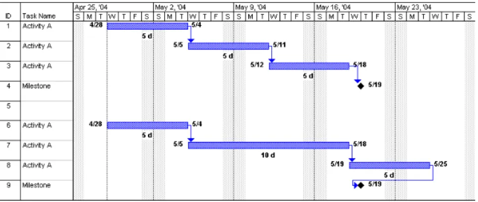
Misuse or overuse of constraints can lead to false conclusions. The constraints that cause the most problems are Must Start On and Must Finish On. These constraints fix a date of the schedule and if earlier durations change, these dates will remain the same and can cause negative slack. Negative slack may mask the critical path of the schedule and is often caused by Finish-to-Finish relationships being used in the wrong order. Negative slack can also be generated when the preceding activity pushes against a date that cannot slip. Other constraints that can cause problems are the Finish or Start No Later Than; they prevent the schedule from reacting appropriately to actual performance. For example, if there is a chain of activities leading to a milestone that is constrained with one of the constricting constraints and one of the durations increases, the milestone will not move and negative slack is created.

Figure 1: Improperly Constrained Milestone

We have developed several quality indices, to help in the assessment of schedule’s quality. These indices look at the ratio of the work tasks to total task, the ratio of work activities with predecessors to total activities, and the ratio of summary tasks without logic to the total number of summary tasks. While we can use these indices to make general assessments as to the quality of the schedule, inspection of individual elements of the schedule may be required to determine whether or not there are specific issues or errors.

KEY SCHEDULE METRICS

We use six key metrics to determine the performance of the effort. It is important to look at both the actual numbers and also the trend over time. Specifically, these metrics are:

1. Work Completed vs. Work Remaining 2. Growth in Work Scheduled

3. Number of Activities on the Critical Path

4. Number of Activities within 20 days of the Critical Path 5. Number of Activities behind schedule

(5)

We use data taken from a typical program to illustrate use for examples. The data can be communicated in several different formats. It can be written in a narrative format or in tabular format. Since we are comparing data against pervious data for the same type in addition to being interested in the trend of the data we have found that the histogram is usually the best method to display the data.

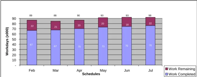
Work complete versus work remaining

In this metric we are comparing the total work planned on the project and then breaking in down into its two basic parts the amount of the work that has been completed and the amount of work that is remaining on the project.

67

67 70 73 75 76

22 ₂₁ 20 20 18 22

-10 20 30 40 50 60 70 80 90

Feb Mar Apr May Jun Jul

Schedules

W

o

rkd

a

y

s

(x00

0)

Work Remaining Work Completed

89 88 90 93 93 98

67

67 70 73 75 76

22 ₂₁ 20 20 18 22

-10 20 30 40 50 60 70 80 90

Schedules

W

o

rkd

a

y

s

(x00

0)

Work Remaining Work Completed

89 88 90 93 93 98

Figure 2: Work Completed And Estimated Work Remaining By Reporting Period

Based on the data in Figure 2, we can use this metric to determine the following. The total number of workdays has been growing slightly for the first five months and then in the last month the growth of the total work increased by 5000 workdays. Between June and July the work completed was only 1000 workdays but the work remaining has increased 4000 workdays. This indicates that more work is being added to the schedule than is being completed. Watching the trend over time would indicate to the project manager that the completion of the project could push to the right.

Growth in Work Scheduled

Taking a more in depth look at part of the information from the previous metric we need to look more closely at the net amount of work that has been added to the schedule. If the growth is positive then the completion of the schedule is going to slip or the addition of labor to complete the efforts on time is going to drive the cost up. We are looking at the net change because work can be deleted from activities just as it can be added to an activity. Figure 3 shows the growth in work scheduled over a six-month period.

(6)

86,785

84,571

86,642

91,287 92,202

98,125

75,000 80,000 85,000 90,000 95,000 100,000

W

o

rk D

ays

Figure 3: Growth In Work Scheduled

As can be seen in this example, the growth increases each month and appears to be growing at an increasing rate since March. This indicates that the contractor may be encountering technical problems or that the original schedule was incomplete and did not include all of the required tasks to complete the program or that the original tasks were underestimated. The analyst must be careful that the duration contained in the summary tasks is not included in the totals for the work planned.

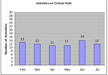
Number of Activities on the Critical Path

Another metric is the number of activities on the Critical Path. The critical path in this case is defined as activities with float less than or equal to zero. Over time the number of activities on the critical path should decrease. If the number stays the same then activities are not being completed or as activities are completed new ones are being added. If this number grows each month it indicates that work is not being accomplished and that the project will finish later than originally planned. Again this number can be adversely affected by negative float or confining constraints.

Activities on Critical Path

13 ₁₂

11 11 12

14

0 2 4 6 8 10 12 14 16 18 20 22 24 26 28 30

N

u

m

b

er

o

f A

c

ti

vi

ti

es

(7)

Figure 4 shows that the number of activities has been fairly constant over a six-month period. Several activities were added in June but the number went do again in July.

Another useful metric is the number of activities that are within 20 days of the critical path. Generally these are the activities that will move to the critical path if activities start to get behind schedule. If this number is large or continues to increase it may mean that activities are being worked in parallel, which increases risk. Many times this metric will give an indication of trouble before the critical path metric.

Activities Behind Schedule

The actual number of activities that are behind schedule (Figure 5) gives management and the analyst a look at the overall health of the program. An activity is behind schedule if the difference between the percent of work complete and the percent that should have been completed based on the status date of the schedule is greater than five percent. We use this five percent as a smoothing factor to account for inaccuracies in the reporting process. If the number of activities behind schedule is large compared to the activities in progress then the analyst might expect the number of activities on or near the critical path to increase, and the risk of completing the project, on time, will increase. This metric along with a list of the activities that are behind schedule will direct attention to areas that are most needed.

Activitie s Be hind S che dule

60

43

3 7

3 3 3 5 3 6

0 10 20 30 40 50 60 70

F e b Ma r Apr May Jun Jul

N

u

m

b

er

o

f A

c

ti

vit

ies

Figure 5: Number Of Activities Behind Schedule

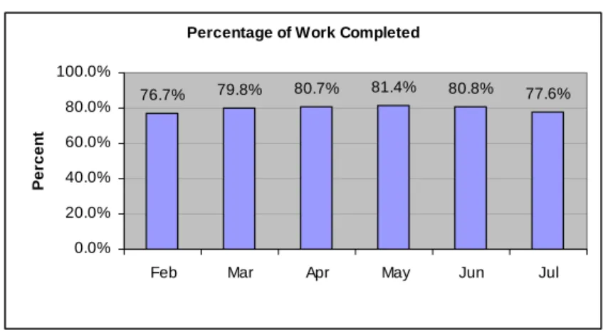
Percent of Work Complete

Another metric used to evaluate the health of a program is the Percent of Work Complete (Figure 6). Ideally this should be a graph with an upward slope. If the trend is otherwise, it may indicate that there is a problem with the program. Additional work may have been added that caused the percent complete on the task to decrease. Work on an activity might have had to be redone and instead of increasing the duration the percent complete it decrease indicating they are not as far along as original thought. The decrease might also been do to a data entry error.

(8)

Percentage of Work Completed

76.7% 79.8% 80.7% 81.4% 80.8% 77.6%

0.0% 20.0% 40.0% 60.0% 80.0% 100.0%

Pe

rc

e

n

t

Figure 6: Percentage Of Work Complete, Overall Program

Referring back to Figure 2, there were more workdays added to the schedule than were completed during the month. This will cause the percent complete on the project to be less than the month before. The slight decrease in June was likely due to rework that was required on several tasks.

Schedule Variance

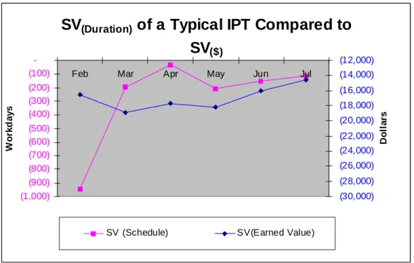
The final metric that will be discussed is the Schedule Variance. This is different from the schedule variance calculated by the Earned Value System (EVS). Using data from the schedule, the schedule variance is determined using the actual work performed compared to the work planned. The details of this process are further explained in the “Using EVM Concepts” section below. This data is then plotted along with the schedule variance from the EVS analysis on the same graph to see if the trends are similar (Figure 7). This provides a crosscheck on the project’s progress from two independent data sources. In many cases the data from the schedule precedes the EVS data by about a month. Actual work performed is determined by multiplying the duration of the activity by the percent of work completed. Planned work is determined by multiplying the duration by the percent of work that should have been completed. The percent of work that should have been completed is the number of workdays from the start of the activity to the status date of the schedule divided by the duration of the activity.

(9)

SV

(Duration)

of a Typical IPT Compared to

SV

($)

(1,000) (900) (800) (700) (600) (500) (400) (300) (200) (100)

-Feb Mar Apr May Jun Jul

Wo

rk

da

y

s

(30,000) (28,000) (26,000) (24,000) (22,000) (20,000) (18,000) (16,000) (14,000) (12,000)

Do

ll

a

rs

SV (Schedule) SV(Earned Value)

Figure 7: Schedule Variance Based On Schedule Data Versus Schedule Data Based On Cost Data

The comparison of the data in Figure 7 shows that with the exception of first data points, the two systems track fairly closely.

To help quantify the schedule performance, we have developed an index that looks at the Schedule Index, similar to the Schedule Performance Index (SPI) from the EVS, calculated from the schedule data, which will be explained later. This is combined with the number of work

activities and milestones that have started compared to the number that should have started. The

third element is the number of activities behind schedule plus the number of missed milestones divided by the number of activities in progress. The three ratios are added together and divided by three to create a single index that ranges between zero and one.

USING EVM CONCEPTS

In order to assist the analyst in collecting the data that is need to analyze the schedule, Tecolote Research, Inc. has developed a tool that assists in the number crunching so the analyst can concentrate on analyzing the data. The Schedule Analyzer does the following:

1. Compares two schedules from the same project together so that the analyst can readily seen the differences

2. Determines what activities are ahead or behind schedule and by how much. 3. Projects ahead to assess the impact on the overall schedule.

(10)

5. Looks at the schedule in the same manner that the EVS does to the budget.

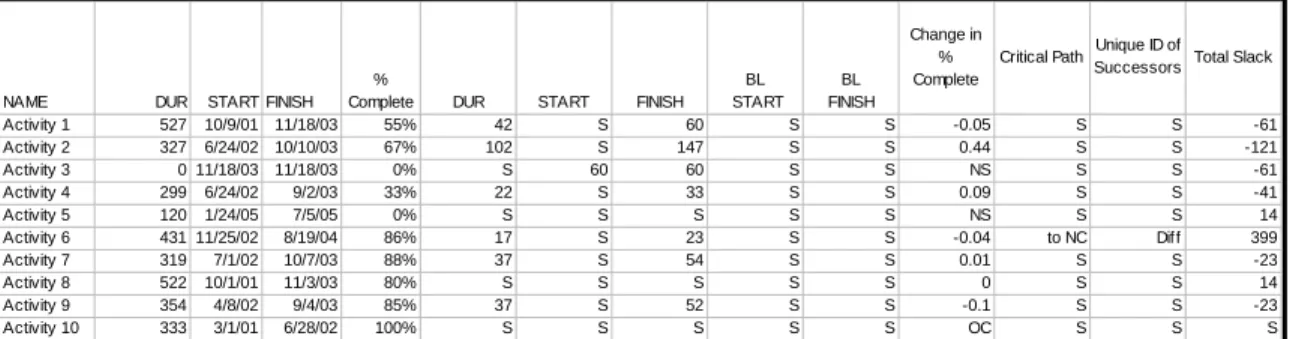
We have developed a procedure to automatically compare two schedules. At a glance, the analyst can determine if there has been a change in the duration of an activity. If the number is negative it means that days were added to the schedule and if the number is positive it indicates that days have been removed from the planned duration. It also compares the Start and Finish dates for both the planned and baseline schedules. A negative value indicates that the date has shifted earlier. When the percent complete data is checked, the analyst can determine if an activity in the latest schedule has increased or decreased and if that activity was completed or started in the current month. The Analyzer compares the critical path from one month to the next and indicates if the activity condition has stayed the same or whether the activity has moved on or off the critical path. It also identifies if there has been a change in logic and if the total slack on the activity changed. Table 1 shows what the data would look like to the analyst. In the table, an “S” indicates a value that has remained the same between the two schedules being compared.

NAME DUR START FINISH %

Complete DUR START FINISH BL START

BL FINISH

Change in % Complete

Critical Path Unique ID of Successors Total Slack

Activity 1 527 10/9/01 11/18/03 55% 42 S 60 S S -0.05 S S -61 Activity 2 327 6/24/02 10/10/03 67% 102 S 147 S S 0.44 S S -121

Activity 3 0 11/18/03 11/18/03 0% S 60 60 S S NS S S -61

Activity 4 299 6/24/02 9/2/03 33% 22 S 33 S S 0.09 S S -41

Activity 5 120 1/24/05 7/5/05 0% S S S S S NS S S 14

Activity 6 431 11/25/02 8/19/04 86% 17 S 23 S S -0.04 to NC Diff 399 Activity 7 319 7/1/02 10/7/03 88% 37 S 54 S S 0.01 S S -23

Activity 8 522 10/1/01 11/3/03 80% S S S S S 0 S S 14

Activity 9 354 4/8/02 9/4/03 85% 37 S 52 S S -0.1 S S -23

Activity 10 333 3/1/01 6/28/02 100% S S S S S OC S S S

Table 1: Comparison Of Key Parameters For Two Schedule Reporting Cycles

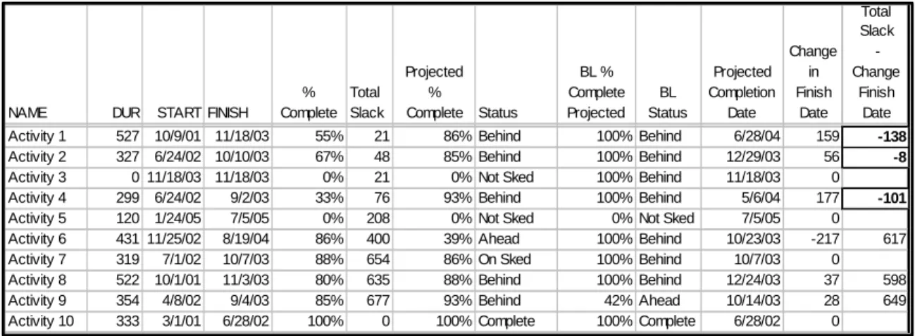
For on-going activities, we calculate the rate of progress for each activity based on the time since the start date and the status date of the schedule to compute a project percent complete for the planned schedule. This is then used to calculate the number of workdays the activity is behind or ahead of schedule. A new completion date is calculated based on the results of that calculation. If the amount that the activity is behind schedule is greater than the slack on the activity, it is flagged as an activity that needs further analysis.

(11)

NAME DUR START FINISH % Complete Total Slack Projected % Complete Status BL % Complete Projected BL Status Projected Completion Date Change in Finish Date Total Slack - Change Finish Date