A systematic approach to offshore wind turbine jacket
predesign and optimization: geometry, cost, and
surrogate structural code check models
Jan Häfele1, Rick R. Damiani2, Ryan N. King2, Cristian G. Gebhardt1, and Raimund Rolfes1
1Leibniz Universität Hannover, Institute of Structural Analysis, Appelstr. 9a, 30167 Hanover, Germany 2National Renewable Energy Laboratory, 15013 Denver West Parkway, Golden, CO 80401, USA
Correspondence:Jan Häfele ([email protected])
Received: 6 May 2018 – Discussion started: 18 May 2018
Revised: 23 July 2018 – Accepted: 6 August 2018 – Published: 23 August 2018
Abstract. The main obstacles in preliminary design studies or optimization of jacket substructures for offshore
wind turbines are high numerical expenses for structural code checks and simplistic cost assumptions. In order to create a basis for fast design evaluations, this work provides the following: first, a jacket model is proposed that covers topology and tube sizing with a limited set of design variables. Second, a cost model is proposed that goes beyond the simple and common mass-dependent approach. And third, the issue of numerical efficiency is addressed by surrogate models for both fatigue and ultimate limit state code checks. In addition, this work shows an example utilizing all models. The outcome can be utilized for preliminary design studies and jacket optimization schemes. It is suitable for scientific and industrial applications.
Copyright statement. The U.S. government retains, and the pub-lisher, by accepting the article for publication, acknowledges that the U.S. government retains a nonexclusive, paid-up, irrevocable, worldwide license to publish or reproduce the published form of this work, or allow others to do so, for U.S. government purposes.
1 Introduction
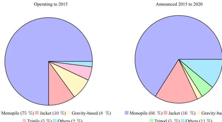
In the oil and gas industry, the jacket substructure is well established due to a good trade-off between cost efficiency and reliability. It has been considered for offshore wind tur-bine substructures for several years and has already had some successful applications in Europe and the United States. Smith et al. (2015) showed that among all wind farms an-nounced to be built from the second quarter of 2015 un-til 2020, 16 % of the substructures are jackets, whereas this share was only 10 % for wind farms built before 2015 (see Fig. 1 for the market shares of offshore wind turbine sub-structures in the past and present). Despite potential advan-tages, the market is still strongly dominated by monopiles (Ho et al., 2016), as financial aspects and significantly lower uncertainty play an important role from an economical point
and turbine parameters on the costs or mass of jackets, con-sidering 81 different structures. Hübler et al. (2017b) ana-lyzed the effect of variations in jacket design on the economic viability. AlHamaydeh et al. (2017) and Kaveh and Sabeti (2018) used meta-heuristic algorithms for the optimization of jacket substructures but without realistic – in particular, fatigue limit state – load assumptions. Stolpe and Sandal (2018) introduced discrete variables in the jacket optimiza-tion problem formulaoptimiza-tion to account for the fact that steel tubes are only available in fixed dimensions.
From a global perspective, the main obstacles that lead to nonoptimal structures are both the dependence on expert knowledge and the large computational cost associated with the optimization of a complex structure. Many design assess-ments or optimization approaches addressing this problem fail (because they lead to either unrealistic or impractical de-sign) for the following simple reasons.
– Design variables. Most approaches do not consider the structural topology, but only the sizing of predefined members. Involving topological parameters, which may be real or discrete, as design variables is mandatory for a proper design that makes use of a mixed-integer for-mulation.
– Cost assumptions. Often, the mass of the entire jacket is used as an objective function in optimization ap-proaches. But obviously, the cost breakdown for a welded structure includes many items that do not de-pend on the mass of the structure. Moreover, other ex-penses such as transport and installation costs should not be ignored.
– Load assumptions. The assumption of simplified envi-ronmental states (for instance, the omission of wind– wave misalignment) is the state of the art in many jacket design procedures because it relaxes the computational demand and fills any existing gap in the knowledge of the actual metocean conditions.
– Structural code checks. A realistic jacket design in-volves structural design code checks for fatigue and ul-timate limit state based on time domain simulations. Many approaches miss either one or both of them, most likely because the computational implementation is re-source intensive.
– Simulation approaches. Design iterations cause changes in the structural behavior. A coupled simulation or at least a rigorous approach addressing this aspect is mandatory. However, it is often seen that sequential approaches are applied when decoupled loads are ex-changed at the interface between substructure and tur-bine tower, even in the case of fatigue assessment.
One possible approach to address some of these issues was the jacket sizing tool proposed by Damiani and Song (2013),
which enables conceptual design by considering preliminary load assumptions. It, however, lacked extensions to full dy-namics simulations and fatigue limit states. Wind turbine cost models are available (Fingersh et al., 2006; National Wind Technology Center Information Portal, 2014) and were used for the definition of wind turbine optimization objectives and constraints (Ning et al., 2013), but without explicit or de-tailed cost formulations for jacket substructures. The goal of the current work is to provide a basic jacket model that can be efficiently used in conceptual studies and optimiza-tion approaches by providing a basis for more realistic de-signs and mainly using mathematically manageable equa-tions. Or, in other words, the main innovation of this study is a basic jacket model that prevents the issues stated above. The first part of this study addresses the first two points de-scribed above. The last three points are handled in the sec-ond part, as they involve a completely different field. This paper is structured as follows: Sect. 2 explains the utilized jacket model with the assumptions made for the structural de-tails. In Sect. 3, a simple cost model is proposed, which cov-ers cost contributions from materials, fabrication, transition piece, coating, and transport and installation (including foun-dation). In Sect. 4, load sets are defined for both fatigue and ultimate limit state load cases and a design of experiments is created to fit appropriate surrogate models. The paper con-cludes with remarks on the benefits of the jacket model, its limitations, and a brief outlook on further work based on this model.
2 Jacket model
The previous section summarized some issues leading to cer-tain requirements of a simple jacket model.
– The set of design variables must be as comprehensive as necessary to accurately model the fundamental topol-ogy, physics, and dynamics of a typical jacket but as small as possible for ease of computation, too.
– The design variables must cover both topological and geometrical parameters.
– Structural details with little bearing on the mechanical behavior shall be disregarded.
– The cost model formulation shall only depend on the parameters of the jacket model.
– The structure shall be manufacturable, transportable, and installable.
– The structure shall be easily transferable to common design tools (mostly based on finite-element formula-tions).
Monopile (75 %) Jacket (10 %) Gravity-based (8 %) Monopile (66 %) Jacket (16 %) Gravity-based (2 %) Tripile (5 %) Others (2 %) Tripod (5 %) Others (11 %)
Figure 1.Share of utilized substructures among operating turbines in 2015 and from 2015 to 2020 according to Smith et al. (2015).
First, the topology is defined; then the tube dimensions and material properties are derived.
2.1 Topology
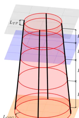
The main presumption is that the jacket model need not be limited to a certain number of legs or brace layers (bays), but instead allows for different topologies. As foot and head girth are measures related to four-legged structures, a general formulation in terms of foot (on the ground layer) and head (on the same layer as the transition piece) circles with foot and head radii RFootandRHead, respectively, is introduced.
In order to prevent obtaining structures with a funnel shape, a parameter,ξ, is introduced, which relates the two radii (and can be set to a value less than or equal to 1). The two cir-cles depict the bottom and top of a frustum of length,L(see Fig. 2a). TheNLlegs can then be constructed as straight lines
on the surface of the cone, equidistantly distributed. This is illustrated for a four-legged jacket in Fig. 2b. However, this procedure is applicable to every number of legs that is greater than or equal to three. With these variables, the angle en-closed by two legs can be found according to the following equation:
ϑ=2π
NL
. (1)
The spatial batter angle,8s, is the inclination angle of each
leg with respect to the symmetry axis of the frustum (some-times denoted as the three-dimensional batter angle):
8s=arctan
Rfoot(1−ξ)
L
. (2)
The planar batter angle,8p, is the inclination angle projected
to a vertical–horizontal layer through the symmetry axis of
the frustum (sometimes denoted as the two-dimensional bat-ter angle):
8p=arctan
Rfoot(1−ξ) sin ϑ2
L
!
. (3)
The parameter,NX, defines the number of bays. A bay is one part of the jacket that is delimited byNLdouble-K joints
at the lower side andNL double-K joints at the upper side
and comprises all structural elements in between, in particu-larNXX joints. Theith bay is denoted withi, where
i∈N[1,NX]. (4)
The ratio,q, relates the heights of two consecutive bays,Li+1
andLi, which is assumed to be constant:
q=Li+1
Li
. (5)
It has to be noted that L1 is the height of the lowest bay
andLNX is the height of the highest one. Based on previ-ous assumptions and elementary geometrical considerations, circles on every double-K joint layer can be constructed. With the height of the entire jacket,L, the distance between the ground and lowest bay,LOSG, and the distance between
the transition piece and highest bay,LTP, theith jacket bay
height,Li, can be calculated by
Li=
L−LOSG−LTP
PNX n=1qn−i
. (6)
The radius of each bay (at the lower double-K joint layer),
Ri, is
Ri=Rfoot−tan (8s) LOSG+ i−1
X
n=1
Ln !
This step is shown in Fig. 2c. The distance between the lower layer of double-K joints and the layer of X joints for theith bay,Lm,i, can be calculated by simple geometrical relations:
Lm,i=
LiRi
Ri+Ri+1
. (8)
The radius of theith X joint layer is
Rm,i=Rfoot−tan (8s) LOSG+ i−1
X
n=1
Ln+Lm,i !
. (9)
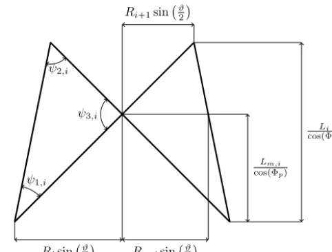
The lower and upper brace-to-leg connection angles,ψ1,iand
ψ2,i, respectively, and the brace-to-brace connection angle,
ψ3,i, in the ith bay are related by trigonometrical relations (see Fig. 3):
ψ1,i=
π
2 −arctan
Rfoot(1−ξ) sin ϑ2cos 8p
L
!
−arctan Lm,i
Risin ϑ2
cos 8p
!
, (10)
ψ2,i=
π
2 +arctan
Rfoot(1−ξ) sin ϑ2cos 8p
L
!
−arctan Lm,i
Risin ϑ2cos 8p
!
, (11)
ψ3,i=2 arctan
Lm,i
Risin ϑ2cos 8p
!
. (12)
In addition,LMSLis the distance between the transition piece
(which is at the same height as the tower foot) and mean sea level layer or, in other words, the difference between jacket length and water depth. This information is necessary to cre-ate a mesh for the computation of hydrodynamic loads. The flag, xMB, determines whether the jacket is equipped with
mud braces or not. The final topology is illustrated in Fig. 2d, in this example with four legs (NL=4), four bays (NX=4), and a mud brace (xMB=true).
2.2 Tube dimensions
The proposed jacket model makes no use of prefabricated joints (as in the state of the art), and no joint cans or stiffen-ers (mainly to improve punching shear resistance) are used. The consequences of only single-sided welds and no stiff-ened joints should be considered. However, the number of (expensive) welds is reduced to a minimum, which reduces the number of degrees of freedom in a structural analysis as well. Moreover, the cost model is not burdened by possible impacts of series manufacturing for prefabricated joints. This is not far away from practical application: it was analyzed for substructures with a rated power higher than 10 MW in the research project INNWIND.EU and evaluated as the most ef-ficient one concerning fabrication costs (Scholle et al., 2015).
Instead of regarding the diameters and thicknesses of each tube as independent variables, which would lead – depending on the structural topology – to a high number of design vari-ables, the tube dimensions are interpolated between values at the top and the bottom of the structure. Another potential problem is that the tube dimensions, if all are regarded as independent, might lead to undesirable relations between the tube dimensions. Standards and guidelines provided by DNV GL AS (2016b, a) for the design and certification of offshore structures propose the adoption of three ratio parameters ini-tially defined by Efthymiou (1988). However, one variable has to be independent; in our case, it is the leg diameter,DL,
which is assumed to be constant.
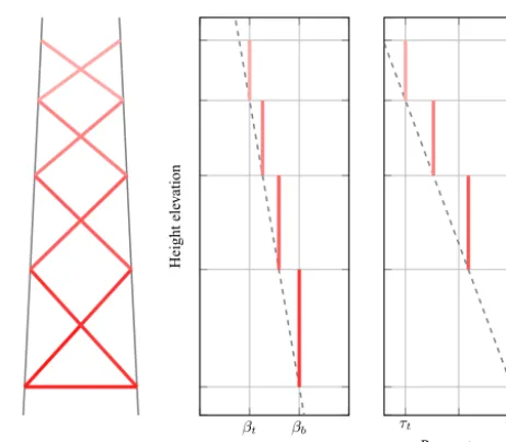
γbandγtdefine the ratios between leg radii (not the
diam-eters) and thicknesses:
γb=
DL
2TLb
, (13)
γt=
DL
2TLt
, (14)
where the indexb indicates the affiliation to the lowermost (bottom) andtto the uppermost (top) tubes. The parameters
βbandβt define the ratios of brace and leg diameter at the
bottom and top, respectively:
βb=
DBb
DL
, (15)
βt=
DBt
DL
. (16)
The valuesτbandτtdefine the relations between brace and
leg thicknesses at the bottom and top, respectively:
τb=
TBb
TLb
, (17)
τt=
TBt
TLt
. (18)
The final determination of the leg and brace dimensions as functions of the height elevation is illustrated in Figs. 4 and 5. The valuesγi,βi, andτican be calculated as follows:
γi=
γb, i=1
(γt−γb)
LOSG+Pin−=11Ln+Lm,i
L−LNX+Lm,NX−LTP +γb else,
(19)
βi=
βt−βb
L−LNX−LOSG−LTP i−1
X
n=1
Ln+βb, (20)
τi=
τt−τb
L−LNX−LOSG−LTP i−1
X
n=1
Ln+τb. (21)
RF oot
RHead
L
(a) Truncated cone defined byRF oot,RHead, andL (b) CreatingNLjacket legs, here:NL= 4
LOSG
LT P
L1
L2
L3
L4
(c) CreatingNX+ 1K-joint layers, here:NX= 4 (d) Final jacket with braces
Figure 2.Creation of the jacket topology in four steps.
height of the X joints. Steps ofβi andτi are located on the height of the double-K joints in order to enable the use of constant tube sizes in each bay.
2.3 Material properties
Figure 3.Theith jacket bay topology projected to the layer of X and double-K joints on one side of the structure.
modulus,E, the shear modulus,G, and the material density,
ρ.
2.4 Parameter summary and array of design variables There are 20 parameters of the jacket model in total: 10 de-scribe the topology, 7 the tube dimensions, and 3 the ma-terial properties. It can be assumed that site- and mama-terial- material-dependent parameters are commonly predetermined, so the number of free design variables might be smaller than 20. To ease the notation in what follows, all variables of the jacket model are assembled in the arrayx:
x=(NL NX Rfoot ξ L LMSL LOSGLTP xMB
q DLγbγtβbβt τbτt E G ρ)T. (22)
3 Cost modeling
A possible approach to the jacket substructure cost calcula-tion is to regard the total capital expenses,Ctotal, as a linear
combination of multiple contributions, with each one given by a cost factor,cj, multiplied by the corresponding unit cost
aj:
Ctotal(x)=
X
ajcj(x) | {z } Cj(x)
. (23)
Basic factors for material, fabrication, coating, transition piece, structural appurtenances (if regarded as additional parts), and transport and installation (including costs for the pile foundation) are assumed here, acknowledging that this breakdown may look different if increasing the level of detail.
c1: material factor
c2: fabrication factor
c3: coating factor
c4: transition piece factor
c5: transport factor
c6: foundation and installation factor
c7: fixed expenses factor
3.1 Material expenses
The material expenses are supposed to be proportional to the mass of the components. Therefore,c1is the total jacket
mass, which is the mass of the assembled substructure ex-cluding the transition piece, foundation, or appurtenances of any kind and which can be obtained by evaluating structural analysis tools or by applying simple geometrical relations from the jacket topology (Fig. 3). The latter can be expressed as a sum:
c1(x)=
2ρNLπ D2L NX
X
i=1
βiτi 2γi
+ τ
2 i 4γi2
!vu u t
L2i cos2 8
p
+Ri+Ri+12sin2
ϑ 2
| {z }
Mass of all diagonal braces
+xMBρNLπ DL2 βbτb
2γb + τ
2 b
4γb2 !
2R1sin
ϑ
2
| {z }
Mass of mud braces
+ρNLπ DL2 NX
X
i=1
1 2γi
+ 1 4γ2
i
!
Lm,i cos (8s)
+ 1
2γi+1 + 1
4γ2 i+1
!
Li−Lm,i cos (8s)
!
| {z }
Mass of intermediate leg elements
+ρNLπ DL2 1 2γb+
1 4γb2
! LOSG cos (8s)
| {z }
Mass of intermediate lowermost elements
+ρNLπ D2L 1 2γt
+ 1
4γt2 !
LTP
cos (8s)
| {z }
Mass of uppermost leg elements
. (24)
3.2 Fabrication expenses
Although it can be assumed that fabrication expenses con-tribute significantly to the overall jacket costs, this factor is often neglected because it is difficult to measure. A com-mon approach in practical applications is to assume a pro-portional relation to the cumulated weld volume. In this cost model,c2is the cumulative volume of all structural welds.
With the weld root thickness,t0(given as 3 mm in
German-ischer Lloyd, 2012) and assuming a 45◦weld angle around the entire weld, the sectional weld area can be approximated and multiplied by the weld length, which is the perimeter of the ellipse that is projected to the connected chord surface1;
DL
Leg diameter
Height
ele
vation
γb γt
Parameterγ
Figure 4.Definition of leg dimensions with a dependency on the jacket height. Values are illustrated by darker coloring at the bottom and shade to lighter at the top of the structure.
thus
c2(x)=
2NLπ DL NX X
i=1 βi
D2 Lτi2 8γ2
i
+t0DLτi
2
√
2γi ! s
1 2sin2 ψ
1,i + 1 2 + s 1 2sin2 ψ2,i
+
1 2+
s
1 2sin2 ψ3,i
+
1 2
!!
| {z }
Brace-to-brace and brace-to-leg weld volume
+2xMBNLπ DLβb
D2Lτb2
8γb2
+t0DLτb
2
√
2γb
!
| {z }
Mud brace-to-leg weld volume
+NLπ DL NX X
i=1
DL2min
1 γ2 i , 1 γ2
i+1
8 +
DLt0min
1 γi,
1 γi+1
2√2
| {z }
Leg-to-leg weld volume
. (25)
The equation uses the perimeter of the ellipse that is pro-jected on a plane to calculate the weld length. This is not exactly equal to the real weld length, but simplifies the equa-tion considerably.
3.3 Coating expenses
Coating is necessary to protect the jacket from corrosion and causes non-negligible costs. It is assumed that the entire outer surface area of all tubes is coated after manufacturing and the
βt βb
Parameterβ
Height
ele
vation
τt τb
Parameterτ
Figure 5.Definition of brace dimensions with a dependency on the jacket height. Values are illustrated by darker coloring at the bottom and shade to lighter at the top of the structure.
coating expenses are proportional to the outer surface areac3:
c3(x)=
2NLπ DL NX
X
i=1 βi
s
L2i
cos2 8 p
+(Ri+Ri+1)
2 sin2 ϑ 2 !
| {z }
Outer surface area of all diagonal braces
+xMBNLπ DLβb
2R1sin
ϑ
2
| {z }
Outer surface area of mud braces
+ NLπ DL
L
cos (8s)
| {z }
Outer surface area of all legs
. (26)
The equation assumes that the reduction of the entire outer surface area due to intersecting tubes is negligible.
3.4 Transition piece expenses
Although there are different transition piece types, a stellar-type transition piece is assumed, which connects the upper-most leg ends with straight bars to a center point. In this case, it can be assumed that the costs depend linearly, on the one hand, on the number of legs and, on the other hand, on the head radius; thus the factorc4reads
c4(x)=NLRfootξ. (27)
3.5 Transport expenses
farm site can be roughly measured in terms of a linear mass dependency, and therefore factorsc5andc1are equal:
c5(x)=c1(x). (28)
However, this value (mass after production) is supposed to be slightly different from the wrought mass that is used due to overlapping joints and material removal prior to welding. To simplify the cost calculation, it is assumed that both values are equal.
3.6 Foundation and installation expenses
The foundation is the structural part that provides an inter-face to the seabed. Both the production costs for the founda-tion structures, no matter of which type, and the on-site in-stallation costs depend linearly on the number of legs in our approach. For the sake of simplicity, it is assumed that these costs do not cover costs due to modifications of the struc-tural pile design. They are assembled in the foundation and installation expenses, and the corresponding factorc6reads
c6(x)=NL. (29)
3.7 Fixed expenses
There are costs that cannot be measured in terms of any pa-rameters of the jacket model:
c7(x)=1. (30)
These kinds of costs – in the nomenclature of this work pro-portional to the factorc7– arise for every structure and are
indeed very important for a cost assessment, but have a rather minor impact on design studies or optimization results, as there is no contribution to differential operators. Examples are costs for structural appurtenances, like boat landings and ladders, or production facilities and infrastructure, like scaf-folds or cranes.
4 Surrogate models for fatigue and ultimate limit
state
A general presupposition made in this work is that realistic jacket design necessitates simulation-based proofs to ensure the structural functionality in different limit states. While the proof of serviceability limit state is mostly simple in the case of relatively stiff lattice structures, for which the tubular tower dominates the modal behavior of the entire turbine, the checks for fatigue and ultimate limit state are computation-ally expensive. There are indeed simulation-based optimiza-tion approaches in the literature, but all with very limited de-sign load sets and proposals trying to find efficient load sets or simplifications of load cases.
Recent work showed that Gaussian process regres-sion (GPR) models are appropriate to predict numerically
obtained fatigue damages for two test structures from envi-ronmental state inputs (Brandt et al., 2017). It is thus straight-forward to transfer the same methodology to the prediction of fatigue damages or utilization ratios due to extreme loads for varying jacket designs in the case that the load sets are given. It is also imaginable to apply a classification approach to this type of problem, with the statements “structural code check successful” or “structural code check failed” as out-puts. However, this would limit the imaginable applications, so regression is applied. In the following, a brief introduction to Gaussian process regression is given. For the sake of sim-plicity, the output dimension of the problem is restricted to one, which is a single-output regression problem. The basis for GPR is the Bayesian regression problem:
y=f(x)+e (31)
with
e∼N0, σn2. (32)
We want to make predictions,y∗, for an arbitrary set of (pre-diction) input variables,x∗, based on information gathered from the training set, which is represented by the input ma-trix, X, and the vector of corresponding output values, y. The key assumption of Gaussian process regression is that a Gaussian distribution overf(x) exists; thus
f(x)∼GP m(x), k(x,x0)
, (33)
with
m(x)=Ef(x) (34)
and
k(x,x0)=covf(x), f(x0), (35)
which is a Mercer kernel function. Due to the marginalization property of Gaussian processes, there is a joint distribution of training and prediction sets:
y y∗
∼
0,
K(X,X) k(X,x∗)
k(x∗,X) k(x∗,x∗)
. (36)
In this equation,Kandkwere introduced to ease the notation and just represent matrices and vectors for which each ele-ment is the corresponding value ofk. The mean of the joint distribution was set to zero. From this equation, the condi-tional posterior distribution ofy∗can be obtained:
y∗|x∗∼N
k(X,x∗)TK(X,X)+σn2I −1
y,
k(x∗,x∗)−k(x∗,X)K(X,X)+σn2I −1
k(X,x∗)
. (37)
because realistic load sets are large and thus the size of the design of experiments is limited. In addition, when the un-certainty arising from design load set assumptions is known, it can be easily considered by an appropriate choice and pa-rameterization of the kernel function.
The prediction of values from a GPR model requires the complete input and output training to set it up. In contrast to the proposed geometry and cost assumptions, the derivation of surrogate models for fatigue and ultimate limit state de-pends highly on the reference turbine and the environmental conditions. The first one has been selected to be the National Renewable Energy Laboratory (NREL) 5 MW turbine, de-fined by Jonkman et al. (2009). The water depth at the fictive location is 50 m. In addition, the research platforms FINO3 (mainly) and FINO1 (for validation purposes) provide de-tailed, long-term measurements to derive the environmental conditions. Soil properties are adopted from the definition of the soil layers in the Offshore Code Comparison Collabora-tion (OC3) project (Jonkman and Musial, 2010). The tran-sition piece is considered with a lumped mass of 660 t at the bottom of the tubular steel tower. There are, however, some limitations in these assumptions that cannot be sup-pressed. No structural appurtenances like ladders, boat land-ings, sacrificial anodes, or J tubes are considered in the struc-tural model. The assumption of 50 m of water depth does not match the water depths at the FINO locations. Nevertheless, no other measurements of environmental states are available, and this assumption was also made in the design basis of the UpWind project (Fischer et al., 2010).
4.1 Training and validation data sets
To obtain training data for surrogate modeling, 200 test jack-ets were sampled from the design space by a space-filling design of experiments with minimum correlation between all samples. Assuming that it is the state-of-the-art reference for 5 MW wind turbine jacket structures, the boundaries in Ta-ble 1 were chosen in a realistic range around the values of the OC4 jacket (Popko et al., 2014), excluding “too optimistic”2 jacket designs. Although the number of samples seems to be low, it has to be considered that the number of time domain simulations depends linearly on the sample size. Moreover, Eq. (37) requires the inversion ofK(X,X), which may lead to weak numerical performance of the prediction. Further-more, an independent validation set with 40 samples from the entire design space was generated, which was created by another space-filling design of experiments. It has to be noted that the purpose of this data set is just validation of the final parameterized models; it is not involved in the training phase and is not part of the cross-validation procedure.
2This statement means that the structural code checks allow wider ranges of the design parameters.
In order to conduct time domain simulations, load sets for both fatigue and ultimate limit state have to be defined. For the fatigue case, broad knowledge about the required size of design load sets is already available because it was analyzed previously in a comprehensive study (Häfele et al., 2017a, b) in which both probabilistic and unidirectional load sets were investigated. However, as the GPR allows us to propagate un-certainties, it is reasonable to utilize a probabilistic load set with 128 production load cases (design load case (DLC) 1.2 and 6.4 according to IEC-61400-3; see International Elec-trotechnical Commision, 2009) for damage estimation (see Table 2), which is a finding of the previously mentioned study. In the extreme load case, the focus is rather on the con-sideration of multiple special events than on the reproduction of the long-term behavior. Table 3 features a summary of all design load cases that are to be calculated for every sample. There are 10 extreme load cases that were identified to be po-tentially critical. DLC 1.3 and 1.6a are production load cases with extreme turbulence and severe sea state, respectively. DLC 2.3 is a design load case for which electrical grid loss occurs during the production state. DLC 6.1a and 6.2a are events with extreme mean wind speed, the first one with an extreme sea state and the second one with an extreme yaw error. The values of the parameters in Table 3 were obtained by evaluating probability density functions of environmen-tal parameters at the FINO locations given by Hübler et al. (2017a).
4.3 Time domain simulations
As the varying jacket design changes the structural behav-ior of the entire turbine, only fully coupled simulations were conducted for this study, as so-called sequential or uncou-pled approaches are considered not sufficiently accurate. All simulations are computed with FAST (National Wind Tech-nology Center Information Portal, 2016) in the current ver-sion at the publication of this study and comprise 10 min time series3plus an additional 3 min time for transient decay. To account for soil–structure interaction, a reduced representa-tion of the substructure (see Häfele et al., 2016) is consid-ered, in which eight interior modes are the basis for the rep-resentation of the jacket with foundation. The pile founda-tion is considered by lumped mass and stiffness matrices at the transition between substructure and ground. These ma-trices are derived by a preprocessing procedure in which the piles withp−y andT−zcurves according to the Ameri-can Petroleum Institute (2002) are discretized with finite el-ements. In the fatigue limit state case, the soil is linearized in the zero-deflection operating point. The operating-point-dependent soil behavior cannot be neglected in the extreme
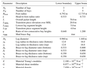
Table 1.Jacket model parameter boundaries for the design of experiments. Topological, tube sizing, and material parameters are separated in groups; single values indicate that the corresponding value is held constant.
Parameter Description Lower boundary Upper boundary
NL Number of legs 3 4
NX Number of bays 3 5
Rfoot Foot radius 6.792 m 12.735 m
ξ Head-to-foot radius ratio 0.533 0.733
L Overall jacket length 70.0 m
LMSL Transition piece elevation over MSL 20.0 m
LOSG Lowest leg segment height 5.0 m
LTP Transition piece segment height 4.0 m
q Ratio of two consecutive bay heights 0.640 1.200
xMB Mud brace flag true
DL Leg diameter 0.960 m 1.440 m
γb Leg radius-to-thickness ratio (bottom) 12.0 18.0 γt Leg radius-to-thickness ratio (top) 12.0 18.0 βb Brace-to-leg diameter ratio (bottom) 0.533 0.800 βt Brace-to-leg diameter ratio (top) 0.533 0.800 τb Brace-to-leg thickness ratio (bottom) 0.350 0.650 τt Brace-to-leg thickness ratio (top) 0.350 0.650
E Material Young’s modulus 2.100×10¹¹N m−2
G Material shear modulus 8.077×10¹⁰N m−2
ρ Material density 7.850×10³kg m−2
Table 2.Considered design load sets according to IEC-61400-3 (International Electrotechnical Commision, 2009) for the fatigue limit state (SF: partial safety factor,vs: mean wind speed,P: probability density function, TI: turbulence intensity,Hs: significant wave height,Tp: wave peak period,θwind: wind direction,θwave: wave direction,uw: near-surface current velocity,uss: subsurface current velocity, MSL: mean sea level). Yaw error is normally distributed with−8◦mean value and 1◦standard deviation.
DLC Quantity Wind Waves Directionality Current Water level
1.2, 6.4
128 vs=P(vs) HS=P(Hs|vs) θwind=P(θwind|vs) uw(0)=0.42 m s −1
MSL SF=1.25 TI=TI(vs) Tp=P(Tp|Hs) θwave=P(θwave|Hs, θwind) uss(0)=0 m s−1
load case and is considered by an ad hoc approach (Hübler et al., 2016).
4.4 Post-processing of time domain results
Fatigue is evaluated in terms of the maximum cumulative damage that occurs in the critical joint after summing up all hot spot damages. AnS−N curve approach defined by the structural code DNV GL RP-0005 (DNV GL AS, 2016a) is utilized for this purpose. Hot spot stresses are obtained by stress concentration factors. Stress cycles are evaluated by a rainflow-counting algorithm and added up according to lin-ear damage accumulation. Fatigue checks are only performed for tubular joints corresponding to classT according to the structural code. The related S−N curve has an endurance stress limit of 52.63×10⁶N m−2 at 107cycles and slopes of 3 and 5 before and after endurance limit, respectively.
Ultimate limit state proofs are performed according to the structural code NORSOK N-004 (NORSOK, 2004), which
is a well-established standard for this purpose. Although the extreme load assessment involves all tubes of the jacket, the output value is only the one with the highest utilization ratio among all considered load cases, including partial safety fac-tors. Punching shear resistance of tubular joints is not consid-ered in the surrogate model because it is not part of the pre-design process. Steel with a yield stress of 355 MPa (S355) is considered as the material for the entire structure, excluding structural appurtenances.
4.5 Derivation and parameterization of Gaussian process regression models
wind direction,θwave: wave direction,uw: near-surface current velocity,uss: subsurface current velocity, MSL: mean sea level). Yaw error is constantly set to−8◦if not stated differently.
DLC Quantity Wind Waves Directionality Current Water level Special event
1.3
1 vs=15.40 m s −1 H
S=2.04 m θwind=0◦ uw(0)=0.42 m s−1 MSL SF=1.35 TI=58.10 % Tp=7.50 s θwave=0◦ uss(0)=0 m s−1
1.3
1 vs=15.40 m s −1 H
S=2.04 m θwind=15◦ uw(0)=0.42 m s−1 MSL SF=1.35 TI=58.10 % Tp=7.50 s θwave=15◦ uss(0)=0 m s−1
1.3
1 vs=17.40 m s −1 H
S=2.50 m θwind=0◦ uw(0)=0.42 m s−1 MSL SF=1.35 TI=44.22 % Tp=7.50 s θwave=0◦ uss(0)=0 m s−1
1.6a
1 vs=11.40 m s −1 H
S=10.60 m θwind=0◦ uw(0)=0.42 m s−1 MSL SF=1.35 TI=8.09 % Tp=15.09 s θwave=0◦ uss(0)=0 m s−1 +2.02 m
2.3
1 vs=25.00 m s −1 H
S=4.63 m θwind=0◦ uw(0)=0.42 m s−1
MSL Grid loss SF=1.1 TI=8.09 % Tp=10.47 s θwave=0◦ uss(0)=0 m s−1
2.3
1 vs=25.00 m s −1 H
S=4.63 m θwind=60◦ uw(0)=0.42 m s−1
MSL Grid loss SF=1.1 TI=8.09 % Tp=10.47 s θwave=60◦ uss(0)=0 m s−1
6.1a
1 vs=42.14 m s −1 H
S=4.63 m θwind=0◦ uw(0)=1.88 m s−1 MSL SF=1.35 TI=12.47 % Tp=10.47 s θwave=0◦ uss(0)=0.69 m s−1 +2.74 m
6.2a
1 vs=42.14 m s −1 H
S=4.63 m θwind=0◦ uw(0)=1.88 m s−1 MSL Yaw error SF=1.1 TI=12.47 % Tp=10.47 s θwave=0◦ uss(0)=0.69 m s−1 +2.74 m 60◦
6.2a
1 vs=42.14 m s −1 H
S=4.63 m θwind=0◦ uw(0)=1.88 m s−1 MSL Yaw error SF=1.1 TI=12.47 % Tp=10.47 s θwave=0◦ uss(0)=0.69 m s−1 +2.74 m 90◦
6.2a
1 vs=42.14 m s −1 H
S=4.63 m θwind=0◦ uw(0)=1.88 m s−1 MSL Yaw error SF=1.1 TI=12.47 % Tp=10.47 s θwave=0◦ uss(0)=0.69 m s−1 +2.74 m 120◦
in terms of cross-validations in this section. Due to the highly nonlinear character of the utilized structural codes and there-fore significant variance in the model outputs, a certain extent of uncertainty has to be tolerated. For the learning procedure, the fatigue damages are logarithmized because the underly-ingS−N curve is also logarithmic and the range of values covers at least 4 powers of 10. For the ultimate limit state, results cover only a range from zero to about 3, and no nor-malization is necessary. However, to exclude severe outliers from the training set of the surrogate model for the ultimate limit state, 10 % of the samples with the highest extreme load utilization ratios are excluded.
The problem of choosing the right kernel function is dis-cussed by many authors. In order to limit the extent of this section, the reader is referred to the works of Duvenaud (2014) and King (2016) for further details. In general, the kernel choice implies a belief about the shape or smoothness of the covariance. In this case, four commonly used station-ary kernel functions are compared that represent relatively smooth approximations of the function.
The squared exponential kernel reads
kSE(x,x0)=exp
−(x−x
0)(x−x0)T
2l2
. (38)
The Matérn 3/2 kernel is
kMa3/2(x,x
0)= 1+ p
3(x−x0)(x−x0)T
l
!
exp −
p
3(x−x0)(x−x0)T
l
!
, (39)
the Matérn 5/2 kernel is
kMa5/2(x,x
0)= 1+ p
5(x−x0)(x−x0)T
l
+5(x−x
0)(x−x0)T
3l2
exp −
p
5(x−x0)(x−x0)T
l
!
and the rational quadratic kernel is
kRQ(x,x0)=
1+(x−x
0)(x−x0)T
2al2
a
, (41)
wherel is a length scale anda a weighting parameter. It is best practice to choose different scales for all input parame-ters. This is called automatic relevance determination (Duve-naud, 2014).
The squared exponential kernel is a common choice for Gaussian processes as an “initial guess” because it is in-finitely differentiable and therefore very smooth. The Matérn kernels are less smooth than the squared exponential kernel: Matérn 3/2 is once and Matérn 5/2 twice differentiable. The rational quadratic kernel is a sum of squared exponential ker-nels with the capability to weight between large- and small-scale variations. To figure out which kernel function is most suitable for both surrogate models, various cross-validations are performed. An N-fold cross-validation means that the training data set (which comprises 200 jacket samples in the fatigue limit state case and 180 samples in the ultimate limit state case in this study) is divided into N parts with equal size. N−1 parts are then used to train the model and the leftover is the test set, which is used to predict a vector of validation results, y∗. This is repeatedN times to compute the mean of the two common error measures, biasebiasand
mean squared erroremse:
ebias=
1
N
N X
n=1
1
M
M X
m=1
y∗n,m−yn,m
!
, (42)
emse=
1
N
N X
n=1
1
M
M X
m=1
y∗n,m−yn,m2 !
, (43)
where y∗
n,m is themth predicted element in the nth cross-validation set andyn,mis the corresponding value in the out-put vector.Mis the size of the cross-validation leftover. For instance, in the case of a 10-fold cross-validation,Mis 20. While the mean squared error is always positive, the bias can have both positive and negative values. Table 4 shows valida-tion results for the four kernels using leave-one-out, 10-fold, and 5-fold cross-validations. There are no values completely off and all kernel functions lead to similar results in the fa-tigue limit state case; the Matérn 5/2 function is eventually chosen for both surrogate models.
4.6 Validation of Gaussian process regression models Based on the kernel function selection, the surrogate mod-els are validated with 40 samples from the design space given in Table 1. A Matérn 5/2 kernel with independent hyperparameters and a Gaussian likelihood function with
lnpσ2 n
= −2.06, where pσ2
n is the mean standard devi-ation of logarithmized damage per load case accounting for load set reduction uncertainty evaluated from the results by
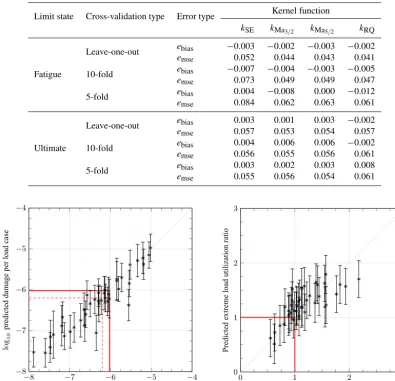
Häfele et al. (2017a, b), are chosen for the fatigue case. The ultimate limit state case does not incorporate prior knowl-edge of uncertainty because it is assumed that one of the con-sidered load cases in Table 3 is the severest imaginable one. The predicted validation values for both fatigue and ultimate limit state are shown in Fig. 6. Although the drawn whiskers show quite wide prediction intervals, the mean values predict the calculated ones well in both diagrams. Therefore, it can be stated that Gaussian process regression is suitable for this task.
5 Example
Although the focus of this work shall not be a comprehen-sive design study, a short example is provided in this section, which shows how the proposed models can be used in further studies.
We assume that for a fixed wind farm location with 50 m of water depth, NREL 5 MW turbine, FINO3 environmen-tal conditions, and OC3 soil properties, it has to be evalu-ated which of three given jacket designs is most suitable with regard to capital expenses. There is uncertainty in the capi-tal expenditures arising from, for example, the market situ-ation, the availability of fabrication facilities and ships, the distance of the installation site from shore, the weather situa-tion, and the sea state. For the sake of simplicity, we assume that this uncertainty can be described in terms of normally distributed cost model parameters given as mean values and standard deviations in Table 54. The parameter distributions indicate relatively high uncertainty, in particular in the penses for transport and installation, which is a common ex-perience in the wind farm planning process. There are three substructure options to be compared: the first (a), derived from the so-called OC4 jacket (Popko et al., 2014), and sec-ond (b) ones are four-legged (NX=4) jackets, and the third (c) one is a three-legged (NX=3) structure. All structures have a length ofL=70 m with transition pieceLMSL=20 m
above mean sea level and use steel (E=2.100×10¹¹N m−2,
G=8.077×10¹⁰N m−2,ρ=7.850×10³kg m−3) as the ma-terial. The height between the ground and lowermost double-K joint layer isLOSG=5 m, and the transition piece height is
LTP=4 m. Furthermore, all jackets have mud braces (xMB=
true); the foot radii,Rfoot, are all 8.485 m, the bay height
ra-tio,q, is 0.8, and the head-to-foot radius ratio,ξ, is 0.67. The leg radius-to-thickness and the leg-to-brace thickness ratios are held constant at γ=γb=γt=15.0 and τ =τb=τt=
0.5, respectively. The structures differ, except for the num-ber of legs (NL), in the number of bays (NX) and tube di-mensions (DL,βb,βt). The first one (a) has four bays, a leg
Limit state Cross-validation type Error type Kernel function
kSE kMa3/2 kMa5/2 kRQ
Fatigue
Leave-one-out ebias −0.003 −0.002 −0.003 −0.002
emse 0.052 0.044 0.043 0.041
10-fold ebias −0.007 −0.004 −0.003 −0.005
emse 0.073 0.049 0.049 0.047
5-fold ebias 0.004 −0.008 0.000 −0.012
emse 0.084 0.062 0.063 0.061
Ultimate
Leave-one-out ebias 0.003 0.001 0.003 −0.002
emse 0.057 0.053 0.054 0.057
10-fold ebias 0.004 0.006 0.006 −0.002
emse 0.056 0.055 0.056 0.061
5-fold ebias 0.003 0.002 0.003 0.008
emse 0.055 0.056 0.054 0.061
−8 −7 −6 −5 −4
−8
−7
−6
−5
−4
log10calculated damage per load case
log
10
predicted
damage
per
load
case
0 1 2 3
0 1 2 3
Calculated extreme load utilization ratio
Predicted
extreme
load
utilization
ratio
(a) (b)
Figure 6.Prediction results for all samples of the validation set. Asterisks depict mean predicted damages in the first and mean extreme load utilization ratios in the second plot, and whisker ranges illustrate the 95 % significance intervals. The solid red line illustrates the critical damage related to a 20-year lifetime of the structure or a utilization ratio of 1. Moreover, the 30-year damage is illustrated with a dashed red line in the first plot.
diameter of 1.2 m, andβ=βb=βt=0.67. The second one
(b) has only three bays, but higher tube diameters and thick-nesses withDL=1.32 m and constantβ=βb=βt=0.75.
The third jacket (c) is the same as the first one (a), but with only three legs (NL=3) and an increased leg
diame-ter DL=1.44 m. Thus, all structures are representative for
different approaches known from practical applications and it is easily imaginable that they differ in all cost factors of the cost model except for the fixed expenses.
First, the cost contributions C1. . .C7 are calculated for
each substructure according to the proposed cost model. Now, two helpful properties are used to evaluate the costs:
Table 5.Reference unit costs for the considered example, a 5 MW reference turbine in a water depth of 50 m.
Unit cost Unit Mean Standard deviation
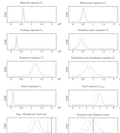
Figure 7.Probability density functions (PDFs) of the cost contributionsC1. . .C7, the total expensesCtotal, the (logarithmized) predicted damage per load case, and the predicted extreme load utilization ratio for the considered example case. Each plot shows the probability density depending on cost, damage exponent, and utilization ratio. Structure (1) is illustrated by the solid gray line, structure (2) by the dashed gray line, and structure (3) by the dotted gray line. The solid red line illustrates the critical damage related to a 20-year lifetime of the structure or a utilization ratio of 1. Moreover, the 30-year damage is illustrated with the dashed red line.
1. the total costs of each substructure,Ctotal, which are a
linear combination of the single contributions,C1. . .C7,
and
2. the sum of normal distributions is again normally dis-tributed.
Figure 7 shows the resulting probability density functions of all cost contributions and the total expenses when the nor-mally distributed unit costs in Table 5 are combined with the proposed cost model. The three-leg design (c) is the cheapest
among the considered structures because the tube dimension increase of 20 % (all tube sizing parameters depend linearly on the leg diameter) is overcompensated for by the reduc-tion in jacket legs, which shows in the factor mass, resulting in significantly lower costs. The structures (a) and (b) show stronger similarities in all cost contributions, adding up to nearly equal total expenses.
pre-structure (c) 10−6.72, all with similar variance. Linear
dam-age accumulation (implying that the lifetime is reached at a cumulated damage of 1) and a simulation time per load case of 10 min yields lifetimes of approximately 100, 155, and 100 years for the three structures, considering a fatigue safety factor of 1.25. The same procedure is applied to ulti-mate limit state assessment and mean tube utilization ratios of 1.05, 0.72, and 0.94 are obtained in the critical load case for the structures (a), (b), and (c), respectively. Therefore, al-though all structures are quite close to an ideal utilization ra-tio, the second structure has the highest capacity concerning extreme loads.
Although only three designs were considered in this ex-ample, it is conceivable that three-legged structures are truly competitive with respect to the given boundaries because the design of structure (c) is related to the lowest capital ex-penses and has sufficient load capacities in the fatigue and ultimate limit state. According to the proposed cost model, the cost saving arises mainly from two contributions, namely transition piece expenses and foundation and installation ex-penses, both depending linearly on the number of jacket legs. This is in agreement with experiences from practical applica-tions because three-legged structures have recently increased in importance, which is visible in the number of offshore in-stallations for turbines with intermediate rated power. Com-paring structure (a) and (b), the cost differences are marginal, while structure (b) turns out to be much better in terms of structural properties, which is visible in a higher lifetime and a lower extreme load utilization ratio. Therefore, it can be stated that the number of jacket legs and the leg diameter (in the case of dependent brace dimensions) are key parameters in the first phase of jacket design. A quantitative sensitivity analysis of the remaining parameters has to be conducted in forthcoming studies.
It can be imagined that the approach is easily usable for far more complex studies in which the number of design samples is much higher than in the present example because the entire procedure, which usually requires enormous nu-merical capacity, was solved in a negligible amount of time. It was already discussed that every jacket design requires a high number of time domain simulations to perform struc-tural code checks. Therefore, the proposed methodology is appropriate to assess the topology and dimensions of a sub-structure, while structural details still have to be determined with high-fidelity models.
Moreover, the example shows that uncertainty can be eas-ily incorporated in the design assessment using the proposed models for capital expenses and structural code checks. This may lead to probabilistic studies or robust jacket design.
The models established in this work provide the groundwork to regard the jacket design process from a scientific point of view, not from an application-oriented design perspective, which depends highly on (human) expert knowledge. This aspect is emphasized strongly at this point because the out-come from studies based on these models will most likely not represent the geometry of the final structure, but an initial or conceptual design approach suitable for implementations with high numerical demands. Therefore, although the pro-posed models provide a comprehensive basis for design eval-uations or optimization, they have to be used with caution. There is still a distinct amount of uncertainty in the surrogate model outputs, which arises from different sources, such as load set reductions, relatively small training sets (due to lim-ited numerical capacity), or nonlinearities in physical models or structural code checks.
In addition, it has to be mentioned that though the methods are probably applicable to other turbines as well, the numeri-cal parameters and results in the considered example are only valid for a jacket substructure at a given (fictive) offshore lo-cation with a 50 m water depth, FINO3 environmental condi-tions, and the NREL 5 MW turbine. An adaption to different boundaries requires a reestimation of the parameters.
7 Conclusions
The objective of this work was to provide a minimal but comprehensive approach to conceptual studies on jacket sub-structures for wind turbines. For this purpose, a geometry model was defined. A completely analytical cost model was derived afterwards. The issue of computationally expensive structural code checks was faced by surrogate modeling, namely Gaussian process regression models. Finally, an ex-ample was considered to show the capabilities of the devel-oped models in which three artificial structures were ana-lyzed. It was shown that different jacket design approaches (varying in topology and tube dimensions) may be appro-priate solutions for a given wind turbine and environmental conditions. The present work improves the state of the art by combining a jacket model with topological design variables, more realistic cost and load assumptions, structural design code checks, and coupled time domain simulations in one approach.
of-ten neglects structural topology aspects, a correct cost as-sessment, or realistic structural code checks. In particular, the utilization of surrogate modeling is very promising when dealing with meta-heuristic algorithms like evolutionary or swarm-based approaches applied to the jacket optimization problem because the related numerical expenses are signifi-cantly lower compared to approaches based on time domain simulations. This may lead to much more detailed analyses of the optimization procedure from the mathematical point of view because approaches known from the literature are fo-cused on technical aspects. Questions to be answered in this
context are, for instance, how the constraints can be handled efficiently or which algorithm is most suitable for the jacket optimization problem.
DLC Design load case
E Expected value
GP(m, k) Gaussian process with mean functionmand covariance functionk
GPR Gaussian process regression MSL Mean sea level
N Set of natural numbers
N(µ, σ2) Normally distributed number with meanµand varianceσ2
SF Partial safety factor TI Turbulence intensity
8p Planar (two-dimensional) batter angle
8s Spatial (three-dimensional) batter angle
βb Brace-to-leg diameter ratio at bottom (jacket model parameter)
βi Brace-to-leg diameter ratio in theith bay
βt Brace-to-leg diameter ratio at top (jacket model parameter)
γb Leg radius-to-thickness ratio at bottom (jacket model parameter)
γi Leg radius-to-thickness ratio in theith bay
γt Leg radius-to-thickness ratio at top (jacket model parameter)
θwave Wave direction
θwind Wind direction
ξ Head-to-foot radius ratio (jacket model parameter)
ρ Material density (jacket model parameter)
σn2 Gaussian input noise variance
ϑ Angle enclosed by two jacket legs
τb Brace-to-leg thickness ratio at bottom (jacket model parameter)
τi Brace-to-leg thickness ratio in theith bay
τt Brace-to-leg thickness ratio at top (jacket model parameter)
ψ1,i Lower brace-to-leg connection angle in theith bay
ψ2,i Upper brace-to-leg connection angle in theith bay
ψ3,i Brace-to-brace connection angle in theith bay
Cj Expenses related tojth cost factor
Ctotal Total capital expenses
DBb Bottom brace diameter
DBt Top brace diameter
DL Leg diameter (jacket model parameter)
E Material Young’s modulus (jacket model parameter)
G Material shear modulus (jacket model parameter)
Hs Significant wave height
I Identity martrix K Kernel function matrix
L Overall jacket length (jacket model parameter)
LMSL Transition piece elevation over MSL (jacket model parameter)
LOSG Lowest leg segment height (jacket model parameter)
LTP Transition piece segment height (jacket model parameter)
Li ith jacket bay height
Lm,i Distance between the lower layer of K joints and the layer of X joints of theith bay
M Size of the cross-validation leftover
N Number of cross-validation bins
NL Number of legs (jacket model parameter)
NX Number of bays (jacket model parameter)
P Probability density function
RHead Head radius
Ri ith jacket bay radius at lower K joint layer
Rm,i Radius of theith X joint layer
TBb Bottom brace thickness
TBt Top brace thickness
TLb Bottom leg thickness
TLt Top leg thickness
Tp Wave peak period
X Matrix of training inputs (one sample per row)
a Kernel weighting parameter
aj jth unit cost
cj jth cost factor
e Noise
ebias Bias error
emse Mean squared error
f Function value
k Kernel function vector
k Covariance (kernel) function
kMa3/2 Matérn 3/2 kernel function
kMa5/2 Matérn 5/2 kernel function
kRQ Rational quadratic kernel function
kSE Squared exponential kernel function
l Kernel length-scale parameter
m Mean function
q Ratio of two consecutive bay heights (jacket model parameter)
uss Subsurface current velocity
uw Near-surface current velocity
vs Mean wind speed
x Array of design variables/vector of training
x∗ Array of prediction inputs
xMB Mud brace flag (jacket model parameter)
y Vector of training outputs (one sample per row)
y General regression output value
Competing interests. The author declares that there is no con-flict of interest.
Disclaimer. The views expressed in the article do not necessarily represent the views of the U.S. Department of Energy or the U.S. government.
Acknowledgements. This work was supported by the compute cluster, which is funded by the Leibniz Universität Hannover, the Lower Saxony Ministry of Science and Culture (MWK), and the German Research Foundation (DFG).
Cordial thanks are given to Jason Jonkman, Amy Robertson, and Katherine Dykes from the National Renewable Energy Laboratory, who supported this work with many valuable remarks and sugges-tions, and Manuela Böhm from Leibniz Universität Hannover for supporting the numerical simulation work.
The Alliance for Sustainable Energy, LLC (Alliance) is the man-ager and operator of the National Renewable Energy Laboratory (NREL). NREL is a national laboratory of the U.S. Department of Energy, Office of Energy Efficiency and Renewable Energy. This work was authored by the Alliance and supported by the U.S. Department of Energy under contract no. DE-AC36-08GO28308. Funding was provided by the U.S. Department of Energy Office of Energy Efficiency and Renewable Energy, Wind Energy Technolo-gies Office.
The publication of this article was funded by the open-access fund of Leibniz Universität Hannover.
Edited by: Athanasios Kolios Reviewed by: two anonymous referees
References
AlHamaydeh, M., Barakat, S., and Nasif, O.: Optimization of Sup-port Structures for Offshore Wind Turbines Using Genetic Al-gorithm with Domain-Trimming, Math. Probl. Eng., 2017, 1–14, https://doi.org/10.1155/2017/5978375, 2017.
American Petroleum Institute: Recommended Practice for Plan-ning, Designing and Constructing Fixed Offshore Platforms – Working Stress Design, Recommended Practice RP 2A-WSD, 2002.
Brandt, S., Broggi, M., Häfele, J., Gebhardt, C. G., Rolfes, R., and Beer, M.: Meta-models for fatigue damage estimation of offshore wind turbines jacket substructures, Procedia Engineer., 199, 1158–1163, https://doi.org/10.1016/j.proeng.2017.09.292, 2017.
BVGassociates: Offshore wind cost reduction pathways – Technol-ogy work stream, Tech. rep., 2012.
BVGassociates: Offshore wind: Industry’s journey to GBP 100/MWh – Cost breakdown and technology transi-tion from 2013 to 2020, Tech. rep., 2013.
tures under fatigue and extreme loads, Mar. Struct., 47, 23–41, https://doi.org/10.1016/j.marstruc.2016.03.002, 2016.
Damiani, R. and Song, H.: A Jacket Sizing Tool for Offshore Wind Turbines within the Systems Engineering Initiative, in: Offshore Technology Conference, 6–9 May 2013, Houston, TX, USA, https://doi.org/10.4043/24140-MS, 2013.
Damiani, R., Dykes, K., and Scott, G.: A comparison study of offshore wind support structures with monopiles and jackets for U.S. waters, J. Phys. Conf. Ser., 753, 092003, https://doi.org/10.1088/1742-6596/753/9/092003, 2016. Damiani, R., Ning, A., Maples, B., Smith, A., and Dykes,
K.: Scenario analysis for techno-economic model develop-ment of U.S. offshore wind support structures: Scenario anal-ysis for techno-economic model development of U.S. off-shore wind support structures, Wind Energy, 20, 731–747, https://doi.org/10.1002/we.2021, 2017.
DNV GL AS: Fatigue design of offshore steel structures, Recom-mended Practice DNVGL-RP-C203, 2016a.
DNV GL AS: Support structures for wind turbines, Offshore Stan-dard DNVGL-ST-126, 2016b.
Duvenaud, D. K.: Automatic Model Construction with Gaussian Processes, PhD thesis, University of Cambridge, Cambridge, UK, 2014.
Efthymiou, M.: Development of SCF formulae and generalised in-fluence functions for use in fatigue analysis, in: Proceedings of the Conference on Recent Developments in Tubular Joints Tech-nology, 1–13, Surrey, 1988.
Fingersh, L., Hand, M., and Laxson, A.: Wind Turbine Design Cost and Scaling Model, Technical Report NREL/TP-500-40566, Golden, CO, USA, 2006.
Fischer, T., de Vries, W., and Schmidt, B.: Upwind Design Basis, Tech. rep., 2010.
Germanischer Lloyd: Guideline for the Certification of Offshore Wind Turbines, Offshore Standard, 3–35, 2012.
GPML: Gaussian process regression models, available at: http: //www.gaussianprocess.org/gpml/code/matlab/doc/, last access: 13 August 2018.
Häfele, J. and Rolfes, R.: Approaching the ideal design of jacket substructures for offshore wind turbines with a Particle Swarm Optimization algorithm, in: Proceedings of the Twenty-sixth (2016) International Offshore and Polar Engineering Conference, Rhodes, Greece, 156–163, 2016.
Häfele, J., Hübler, C., Gebhardt, C. G., and Rolfes, R.: An improved two-step soil-structure interaction modeling method for dynam-ical analyses of offshore wind turbines, Appl. Ocean Res., 55, 141–150, https://doi.org/10.1016/j.apor.2015.12.001, 2016. Häfele, J., Hübler, C., Gebhardt, C. G., and Rolfes, R.: A
com-prehensive fatigue load set reduction study for offshore wind turbines with jacket substructures, Renew. Energ., 118, 99–112, https://doi.org/10.1016/j.renene.2017.10.097, 2017a.
Ho, A., Mbistrova, A., and Corbetta, G.: The European offshore wind industry – key trends and statistics 2015, Tech. rep., 2016. Hübler, C., Häfele, J., Ehrmann, A., and Rolfes, R.: Effective
con-sideration of soil characteristics in time domain simulations of bottom fixed offshore wind turbines, in: Proceedings of the Twenty-sixth (2016) International Offshore and Polar Engineer-ing Conference, Rhodes, Greece, 127–134, 2016.
Hübler, C., Gebhardt, C. G., and Rolfes, R.: Development of a comprehensive database of scattering environmental conditions and simulation constraints for offshore wind turbines, Wind En-erg. Sci., 2, 491–505, https://doi.org/10.5194/wes-2-491-2017, 2017a.
Hübler, C., Piel, J.-H., Breitner, M. H., and Rolfes, R.: How Do Structural Designs Affect the Economic Viability of Offshore Wind Turbines? An Interdisciplinary Simulation Approach, in: Conference: International Conference on Operations Research, Berlin, Germany, 2017b.
International Electrotechnical Commision: Wind turbines – Part 3: Design requirements for offshore wind turbines, Tech. Rep. IEC-61400-3:2009, EN IEC-61400-3:2009, 2009.
Jonkman, J. M. and Musial, W.: Offshore Code Comparison Collab-oration (OC3) for IEA Task 23 Offshore Wind Technology and Deployment, Technical Report NREL/TP-5000-48191, National Renewable Energy Laboratory, Golden, CO, USA, 2010. Jonkman, J. M., Butterfield, S., Musial, W., and Scott, G.:
Defini-tion of a 5-MW Reference Wind Turbine for Offshore System Development, Technical Report NREL/TP-500-38060, National Renewable Energy Laboratory, Golden, CO, USA, 2009. Kaveh, A. and Sabeti, S.: Structural optimization of jacket
support-ing structures for offshore wind turbines ussupport-ing collidsupport-ing bod-ies optimization algorithm, Struct. Des. Tall. Spec., 27, e1494, https://doi.org/10.1002/tal.1494, 2018.
King, R. N.: Learning and Optimization for Turbulent Flows, PhD thesis, University of Colorado, Boulder, CO, USA, 2016. Michels, G.: Mass Production of Offshore Wind-Jackets requires
new Industrial Solutions, in: Nationale Staalbouwdag, Katwijk, the Netherlands, 2014.
National Wind Technology Center Information Portal: Plant_CostsSE, available at: https://nwtc.nrel.gov/Plant_ CostsSE (last access: 23 July 2018), 2014.
National Wind Technology Center Information Portal: FAST v8, available at: https://nwtc.nrel.gov/FAST8 (last access: 23 July 2018), 2016.
Ning, A., Damiani, R., and Moriarty, P.: Objectives and Constraints for Wind Turbine Optimization, in: 51st AIAA Aerospace Sciences Meeting, Grapevine, TX, USA, https://doi.org/10.2514/6.2013-201, 2013.
NORSOK: Design of steel structures, Standard N-004 Rev. 2, 2004. Oest, J., Sørensen, R., T. Overgaard, L. C., and Lund, E.: Struc-tural optimization with fatigue and ultimate limit constraints of jacket structures for large offshore wind turbines, Struct. Mul-tidiscip. O., 55, 779–793, https://doi.org/10.1007/s00158-016-1527-x, 2016.
Popko, W., Vorpahl, F., Zuga, A., Kohlmeier, M., Jonkman, J., Robertson, A., Larsen, T. J., Yde, A., Saetertro, K., Okstad, K. M., Nichols, J., Nygaard, T. A., Gao, Z., Manolas, D., Kim, K., Yu, Q., Shi, W., Park, H., Vasquez-Rojas, A., Dubois, J., Kaufer, D., Thomassen, P., de Ruiter, M. J., Peeringa, J. M., Zhiwen, H., and von Waaden, H.: Offshore Code Comparison Collaboration Continuation (OC4), Phase I – Results of Coupled Simulations of an Offshore Wind Turbine with Jacket Support Structure, Journal of Ocean and Wind Energy, 1, 1–11, 2014. Rasmussen, C. E. and Williams, C. K. I.: Gaussian processes for
machine learning, MIT Press, Cambridge, MA, USA, 3rd print edn., 2008.
Scholle, N., Radulovi´c, L., Nijssen, R., Ibsen, L. B., Kohlmeier, M., Foglia, A., Natarajan, A., Thiel, J., Kuhnle, B., Kraft, M., Kühn, M., Brosche, P., and Kaufer, D.: Innovations on component level (final report), INNWIND.EU Deliverable D4.1.3, 2015. Smith, A., Stehly, T., and Musial, W.: 2014-2015 Offshore Wind
Technologies Market Report, Technical Report NREL/TP-5000-64283, National Renewable Energy Laboratory, Golden, CO, USA, 2015.