https://doi.org/10.5194/gmd-11-4043-2018 © Author(s) 2018. This work is distributed under the Creative Commons Attribution 4.0 License.
ICON-ART 2.1: a flexible tracer framework and its application
for composition studies in numerical weather forecasting
and climate simulations
Jennifer Schröter1, Daniel Rieger1,3, Christian Stassen1,a, Heike Vogel1, Michael Weimer2, Sven Werchner1, Jochen Förstner3, Florian Prill3, Daniel Reinert3, Günther Zängl3, Marco Giorgetta4, Roland Ruhnke1, Bernhard Vogel1, and Peter Braesicke1
1Institute of Meteorology and Climate Research, Karlsruhe Institute of Technology, Karlsruhe, Germany 2Steinbuch Centre for Computing, Karlsruhe Institute of Technology, Karlsruhe, Germany
3Deutscher Wetterdienst, Offenbach, Germany
4Max Planck Institute for Meteorology, Hamburg, Germany
anow at: ARC Centre of Excellence for Climate System Science, School of Earth Atmosphere and Environment, Monash University, Melbourne, Australia
Correspondence:Jennifer Schröter ([email protected]) Received: 8 November 2017 – Discussion started: 22 February 2018
Revised: 23 August 2018 – Accepted: 28 August 2018 – Published: 5 October 2018
Abstract.Atmospheric composition studies on weather and
climate timescales require flexible, scalable models. The ICOsahedral Nonhydrostatic model with Aerosols and Re-active Trace gases (ICON-ART) provides such an environ-ment. Here, we introduce the most up-to-date version of the flexible tracer framework for ICON-ART and explain its ap-plication in one numerical weather forecast and one climate related case study. We demonstrate the implementation of idealised tracers and chemistry tendencies of different com-plexity using the ART infrastructure. Using different ICON physics configurations for weather and climate with ART, we perform integrations on different timescales, illustrating the model’s performance. First, we present a hindcast exper-iment for the 2002 ozone hole split with two different ozone chemistry schemes using the numerical weather prediction physics configuration. We compare the hindcast with obser-vations and discuss the confinement of the vortex split us-ing an idealised tracer diagnostic. Secondly, we study AMIP-type integrations using a simplified chemistry scheme in con-junction with the climate physics configuration. We use two different simulations: the interactive simulation, where mod-elled ozone is coupled back to the radiation scheme, and the non-interactive simulation that uses a default background cli-matology of ozone. Additionally, we introduce changes of water vapour by methane oxidation for the interactive
sim-ulation. We discuss the impact of stratospheric ozone and water vapour variations in the interactive and non-interactive integrations on the water vapour tape recorder, as a measure of tropical upwelling changes. Additionally we explain the seasonal evolution and latitudinal distribution of the age of air. The age of air is a measure of the strength of the merid-ional overturning circulation with young air in the tropical upwelling region and older air in polar winter downwelling regions. We conclude that our flexible tracer framework al-lows for tailor-made configurations of ICON-ART in weather and climate applications that are easy to configure and run well.
1 Introduction
equa-tions (i.e. the acceleration term dw/dtin the vertical momen-tum equation is no longer neglected). In principle, this al-lows the same dynamical core to be applied across the entire range of temporal and spatial scales that exist in the atmo-sphere. Thus, simulations ranging from a few hours to hun-dreds of years may become more consistent and advances of one scale or application can more easily be transferred to another. However, the construction of scale-aware physical parameterisations that can be applied over the entire range of scales remains a challenge (Rauscher et al., 2013; Chun et al., 2016).
The extended modelling system ICON-ART (ICOsahe-dral Nonhydrostatic – Aerosols and Reactive Trace Gases; Rieger et al., 2015) is a representative of a next-generation system. ICON (Zängl et al., 2015) is a joint development of Deutscher Wetterdienst (DWD) and Max Planck Insti-tute for Meteorology (MPI-M). The dynamical core of ICON is based on the nonhydrostatic formulation of the vertical momentum equation. Thus, ICON allows simulations with high horizontal resolutions, up to grid spacings of a few hundreds of metres. However, while the dynamical core of ICON is unified, individual applications like large eddy sim-ulations (LESs), NWP or climate projections, e.g. EC(MWF) HAM(burg) (ECHAM), currently use different parameteri-sations of physical processes (Dipankar et al., 2015; Heinze et al., 2017).
ICON offers the possibility of local grid refinements, also called “nesting”. The nesting provides the option of two-way interactions between the (global) coarse domain and the higher-resolution local domain. Hierarchical nesting and sev-eral domains at the same nesting level are possible. ICON already provides benefits in various application fields, e.g. in the High Definition Clouds and Precipitation for advanc-ing Climate Prediction (HD(CP)2) project. Selected results of the HD(CP)2project are described in Heinze et al. (2017). Within this project, the configuration of the LES physical configuration has been developed and is used to achieve a better understanding of, for example, processes that are re-lated to precipitation. Results will help to improve future cli-mate projections on coarser resolutions.
Since January 2015, ICON has been running operationally at DWD for weather forecasts on the global scale with a grid spacing of 13 km. Since June 2015, a local grid refinement over Europe with a horizontal resolution of 6.5 km has been in operational use as well.
ART is an additional module for ICON, developed at the Karlsruhe Institute of Technology. It contributes to the goal of a unified global next-generation modelling system with a variety of applications in the field of atmospheric com-position sciences. A variant of the ART module is also be-ing used in COSMO-ART. However, parameterisations dif-fer and implementations have been updated to newer Fortran standards. ICON-ART extends the numerical weather and climate prediction system ICON with (gas-phase) chemistry, aerosol dynamics and related feedback processes. A
compre-hensive treatment of feedback processes between chemistry, aerosols, clouds and radiation can now be included in recent and future studies (Gasch et al., 2017; Rieger et al., 2017; Weimer et al., 2017; Eckstein et al., 2017).
Here, we will discuss the unified tracer framework of ICON-ART that allows to define and specify tracer initialisa-tion and a coupling of individual chemical mechanisms and specific process modules. Depending on the requirements of the application field, like large eddy simulations, numerical weather predictions or climate simulations, ICON-ART can run with the different existing physics configurations.
Given the multitude of challenges we are facing, models have to be capable of being readily changed. Therefore, it is of high importance to provide a tracer framework that is flex-ible and suitable for a large variety of different applications. For the development of next-generation modelling systems, the requirements for modern high-performance computer ar-chitectures also have to be considered. Nowadays, numeri-cal models are integrated on massively parallel architectures with up to 106 cores. Unstructured grids like the icosahe-dral ICON grid show advantages regarding the performance on current high-performance computing systems (e.g. Zängl et al., 2015). Taking into account the increase of computa-tional power over the last years, it is obvious that more diag-nostic and progdiag-nostic tracers will be included in future sim-ulations than before. With ICON-ART 2.1, we introduce a new flexible tracer framework, which meets the demands of a next-generation modelling system. There is full flexibility in defining the tracers and associated characteristics. The set of tracers can be tailored for individual experimental setups of different complexity. The model allows for changes in the set of tracers without any recompilation. The ability to replace the common usage of namelist structures, previously used by ICON-ART and other models (e.g. Morgenstern et al., 2017; Baklanov et al., 2014), is fully supported.
Here, we describe the concept of the new ICON-ART tracer framework. The technical description is followed by examples of definitions for chemical and passive tracers in ICON-ART in Sect. 5. In Sect. 5, we give an overview of different applications of ICON-ART using the flexible tracer framework. These applications include simulations with the numerical weather prediction physics configuration and sim-ulations with the climate physics configuration. We finish with some concluding remarks and an outlook.
2 The ICON-ART tracer framework
chemi-cal tracers leading to a less expensive chemi-calculation in terms of computational time. In addition, sometimes chemical tracers with a short lifetime, compared to dynamical timescales, can be neglected in the transport processes.
With ICON-ART, we introduce a flexible tracer framework with a minimum of predefinitions that allows all of the above and more. The user has the ability to define a unique set of tracers, tailored to the requirements of the model experi-ment planned. The new tracer framework builds on structures which are already implemented in the basic ICON frame-work and shared by different available physical configura-tions. These configurations are the LES physics configuration (Dipankar et al., 2015; Heinze et al., 2017), the NWP physics configuration and the climate physics configuration based on ECHAM6 parameterisation (Giorgetta et al., 2018). The new tracer framework allows flexible coupling to the selected physical configuration. Thus, the composition coupling can be performed without subsequent changes. The ART code is not changed when the physics configuration is changed.
This allows an independent investigation of atmospheric processes using different physical configurations.
2.1 Technical description of the tracer framework
The technical framework of ICON-ART is based on Fortran 2008, which provides essential functionality for the new tracer framework. Classes allow to overcome the strin-gent matching of data types. Items only have to match a data type or any extension of this type when it is declared
with CLASS(type) where type is a derived data type
(Chapman, 2008). If theCLASSmatches more than one data type, it is called polymorphic. Within ICON-ART, we are us-ing these polymorphic objects to extend the existus-ing tracer structure by additional metadata. Linked lists are another Fortran 2008 feature that is extensively used. Linked lists al-low for new features like passing a reference to the next list element or adding and deleting elements.
In the scope of this paper, we are working with two differ-ent types of tracers: passive and chemical active ones. An ex-ample for a passive tracer is a constituent that does not have any impact on other tracers or the thermodynamics of the simulated system. Passive tracers have predefined sources or only fixed initial conditions. They change by transport and do not interact with other tracers or processes. Chemical active tracers experience sources and sinks while being transported and can participate in feedback processes.
Passive and chemical active tracers are distinguished by their associated metadata. In our example, passive tracers have no chemical loss term to be considered. In other words, the lifetime of passive tracers is infinite. Information about the lifetime is used for simple chemical tracers that expe-rience an idealised loss while being transported. Of course, the information dealing with transport should be provided for both tracer types. A flexible aerosol dynamics module
mak-ing use of the flexible tracer framework is currently undergo-ing development.
2.2 Storage of metadata information
We extend the existing ICON-ART functionality by the us-age of a key-value storus-age. The storus-age is based on string comparisons using generic hash tables. For every tracer, a unique key of fixed size is defined. This represents the search key. The table is constructed like a dictionary. Tracer infor-mation can be looked up fast, using this search key. Hash tables provide the foundation for a generic and flexible con-cept to read and store metadata. At model initialisation, one key-value storage for each tracer is initialised by
CALL storage%init(lcase_sensitivity=.FALSE.)
In this case, the dictionary entries are not case sensitive. The storage unit has two fundamental subroutines; these
arestorage%putandstorage%get. The first creates
a new dictionary entry, and the second searches for a key and gives the connected entry. In the next step, this storage unit has to be filled. Accepted types of storage values are reals, integers or characters.
2.2.1 Reading in metadata information from XML files
At one point in time, all numerical models need to find an answer to the question how to transfer text-based informa-tion (e.g. tracer metadata) into the model’s program code. The text-based format XML (eXtensible Markup Language) (see W3C-Recommendation, 2017) gives the developer and the user the ability to store and transport information in a structured way.
XML has only few mandatory rules; e.g. there has to be exactly one root element. The framework in which the in-formation is structured can be freely chosen. The structure itself allows for a human readable format. ICON-ART uses the Fortran interface TiXI (https://github.com/DLR-SC/tixi, last access: 27 September 2018) to read the XML file. The TiXI interface includes a flexible mechanism for XML file reading. Since the scripting language of XPath is used, the navigation through an XML document is an easy task to per-form. The XML reading routine can be structured in the same way as someone would read a document and remember the content in the most natural way. An example structure of such an XML input file for the tracer structure is the following:
<?xml version="1.0" encoding="UTF-8"?> <!DOCTYPE tracers SYSTEM "tracers_gp.dtd">
<tracers>
<chemical id="TRO3">
<mol_weight type="real"> 4.800E-2 </mol_weight> <lifetime type="real"> 2592000 </lifetime> <transport type="char"> stdchem </transport> <init_mode type="int"> 0 </init_mode> <unit type="char"> mol mol-1 </unit> <long_name type="char"> ozone </long_name> </chemical>
The XML file is scanned automatically. For the realisa-tion of this feature, it is necessary to predefine the type of input. Every tag has a mandatory type definition, i.e.char, int and real. The first word in brackets,<tracers>, is called XML tag. The tag <chemical id=”TRO3”>
has the additional attribute idfor the tag chemical. To identify a specific tracer, the system uses the given attribute (e.g.id). Tags are used to build up the metadata structure. It is a key-value storage where the tag (e.g.mol_weight) is the key with the value, e.g. 4.800E-2for ozone. The number4.800E-2is then stored in the metadata structure of ICON-ART. At this point, it should be noted that there are two kinds of metadata: necessary and optional metadata. Necessary metadata depend on the polymorphic type. Pas-sive tracers do have different necessary metadata than chem-ical tracers. The optional metadata are read in automatchem-ically. Every tag in the XML file is translated into an entry in the key-value storage.
The structure of the ART tracer framework is shared with the core ICON tracer framework and only expanded in the cases needed. In addition to that, tracers can share attributes and are distinguished by additional attributes. In our exam-ple, ozone appears in two different subroutines for chemistry: the first using a lifetime-based mechanism, and the second using a full gas-phase approach.
The tag <mol_weight> can be used for unit conver-sion within a subroutine and is given in kg mol−1. The tag
<lifetime>is used for simplified integration methods for
a given lifetime of a species, in seconds. Some chemical substances or passive tracers do not have to be transported; thus, the tag<transport>ensures that this information is transferred to the program code and the transport is switched on or off, respectively. In addition to that, templates can be defined. In this case, a template named stdchemis cho-sen. At model startup, this template is translated into a spe-cific selection of horizontal and vertical transport schemes. Each scheme stands for a specific numerical discretisation of the mass continuity equation in horizontal or vertical di-rections. Currently, there are three different default transport templates available:off,stdaeroandstdchem. These templates avoid the necessity of adding a tracer advection scheme and flux limiter for each single tracer in the namelist. Hence, the values of the ICON-ART namelist parameters
ihadv_tracer,ivadv_tracer,itype_hlimitand
itype_vlimitare overwritten by the template. Specific
information concerning the advection schemes mentioned can be found in the official ICON documentation. Specifying
offwill deactivate advective transport for this tracer com-pletely.
The transport templatestdchemuses the same advection schemes asstdaero. However, the considerably faster pos-itive definite flux limiters are used instead of the monotone flux limiter. The conservation of linear correlations is traded for a faster computation of the advection.
If chemical species need to be initialised, this is achieved
via<init_mode>and a respective number corresponding
to the initialisation scheme. If theinit_modeis set to 0, no external initialisation data are used. With integers differ-ent from zero, data from other models, like EMAC (Jöckel et al., 2005) or MOZART (Emmons et al., 2010), interpo-lated on the horizontal icosahedral grid are read in and used. The vertical interpolation is performed online. Thus, the ini-tialisation dataset stays unchanged, regardless of the choice of model levels for the simulation.
The structure of the key-value storage for every tracer is built up automatically. This feature allows for an extensive flexibility which has to be controlled. In our case, attributes are used in a fixed manner; they define our basic framework of the tracer structure. The full flexibility, direct access, con-trol mechanisms and data type distinction are only a few advantages of this XML-based procedure against other cur-rently used strategies.
2.3 Construction of the tracer metadata structure
Within ICON-ART, the metadata, e.g. regarding transport or chemical properties, are read in using the XML interface. Af-terwards, the information is stored in the ICON-ART tracer framework. The individual steps of the tracer transport simu-lation in ICON and ICON-ART are described in Rieger et al. (2015). Figure 1 shows the calling structure of the tracer framework in ICON-ART with regard to the tracer and meta-data construction. All tracers within the ICON-ART tracer framework share a common structure like the following:
TYPE t_tracer_meta ...
END TYPE t_tracer_meta
In the case of chemical tracers, we want to provide addi-tional information on, e.g. mol weight. The extension of the derived type looks like this:
TYPE, EXTENDS(t_tracer_meta) :: t_chem_meta
REAL(wp) mol_weight
END TYPE t_chem_meta
In this case, themol_weightis mandatory information. Optional metadata are stored in as part of the basic structure
t_tracer_meta. This container includes a key-value
stor-age. This solution ensures that the metadata container stays as flexible as possible. The respective XML file is read in, and all information is processed and stored in theopt_meta
container; see Fig. 1. In the example ofmol_weight, this attribute becomes a real variable accessible in the code. It can be accessed by using, e.g.
SELECT TYPE(meta => info_dyn%tracer) CLASS IS (t_chem_meta)
CALL meta%opt_meta%get(’mol_weight’, & & mol_weight, ierror)
art_open_xml_file tracer1 opt_meta%init
tracerN opt_meta%init art_read_elements_xml
tracer1 opt_meta%put(element1, value)
art_tracer_def_wrapper
tracer1 create
tracer_meta = (name = name, mol_weight = mw, transport = transport_template(tra), ...) add_ref(tracer_name, tracer_meta ...)
mo_art_init_gasphase
tracer1
meta%opt_meta%get('number',kpp_ind,ierror) meta%opt_meta%get('init_mode', init_mode, ierror)
IF (init_mode == 1) THEN ....
ENDIF tracer1 opt_meta%put(elementM, value)
Figure 1.Schematic describing the tracer framework and the tracer definition in ICON-ART.
Here, CALL meta%opt_meta%get(. . . ) is the opera-tion to access the key-value storage in the container.
The combination of linked lists, polymorphic classes and key-value storage allows the user to define tracers in a flex-ible way. Only those tracers given in an input file are read in, registered and appear in the modelling system. With this solution, the user is free to define any number of chemical or passive tracers which is only limited by the memory of the computing system.
2.4 Construction of XML tracer input file via MECCA
The XML file can either be edited manually by the user or generated automatically by an external program. The tracer files used for the experiments described in Sect. 5 are shown in Appendix A. In this section, we demonstrate the XML file generation by an external program, which also extends the functionality of ICON-ART. In addition to the existing lifetime-based chemistry approach (see Rieger et al., 2015), a full gas-phase chemistry approach is added.
Construction of the full gas-phase chemistry approach is done using the comprehensive and flexible atmospheric chemistry module MECCA (Module Efficiently Calculat-ing the Chemistry of the Atmosphere; Sander et al., 2011). MECCA provides a set of chemical reactions covering the troposphere as well as the stratosphere. The base version of MECCA is extendable by its own chemical reactions or an update of rate coefficients.
The MECCA preprocessing part has been extended by a routine constructing the XML file for the tracer module of ICON-ART. The numerical flexibility of MECCA is based on the KPP software (Kinetic PreProcessor; Sandu and Sander, 2006). KPP generates Fortran90 code which is used to solve the differential equations based on the given chem-ical reaction. This is the first step which is needed for KPP and thus for MECCA. In a second step, the numerical inte-grator is chosen. For our example, we use the Rosenbrock
solver of the third order (Sandu et al., 1997). In the third step, we use the driver part of MECCA. The driver stands for the main program which calls the integrator, reads in-put datasets and writes the results in the original MECCA model. Within ICON-ART, we replaced this step by routines of ICON and ICON-ART. Only the integrator call element is maintained. A shell script, in combination with the AWK scripting language (Aho et al., 1987) processes all informa-tion and generates the respective files and routines. Techni-cal work has been done to ensure that a dictionary is acces-sible for the translation between four-dimensional chemical tracers in ICON-ART and one-dimensional concentrations of chemical species in the KPP routines.
Additionally, other chemical reaction mechanisms pro-vided by MECCA can be used within ICON-ART without changes in the program code itself. It is sufficient to read the new tracer XML file generated by the MECCA preprocessor. Finally, all standard reaction schemes provided by MECCA are accessible in ICON-ART by only using MECCA as an external preprocessor. The model has to be recompiled once, but the user does not have to perform changes in the program code. Files that are changed by the preprocessor are copied to the respective ICON directory automatically. Photolysis rates are calculated using an updated version of CloudJ7.3 (Prather, 2015).
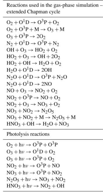
In the scope of this paper, we use a chemical reaction mechanism based on the extended Chapman cycle to demon-strate the functionality of the ICON-ART gas-phase routine.
We defined the chemical reactions as shown in Table 1.
3 Integration of the ART module into ECHAM physics
routines
Table 1.Summary of the chemical reactions used for the extended Chapman cycle simulation.
Reactions used in the gas-phase simulation – extended Chapman cycle
O2+O1D→O3P+O2
O2+O3P+M→O3+M
O3+O3P→2O2
N2+O1D→O3P+N2
OH+O3→HO2+O2
HO2+O3→OH+2O2
HO2+OH→H2O+O2 H2O+O1D→2OH
N2O+O1D→O3P+N2O N2O+O1D→2NO
NO+O3→NO2+O2 NO2+O3P→NO+O2
NO2+O3→NO3+O2 NO3+NO2→N2O5
NO3+NO2+M→N2O5+M
HNO3+OH→H2O+NO3
Photolysis reactions
O2+hν→O3P+O3P
O3+hν→O1D+O2 O3+hν→O3P+O2
NO2+hν→O3P+NO NO3+hν→O3P+NO2
N2O5+hν→NO3+NO2 HNO3+hν→NO2+OH
clear code distinction using compiler directives, described in Rieger et al. (2015), remains the same.
Figure 2 shows a schematic overview of the calling strat-egy of subroutines with the ECHAM (climate) physics con-figuration. Boxes marked partly orange are shared structures between ICON and ICON-ART. Boxes with an orange frame are processes affected by ART tracer tendencies. Boxes with an orange background are ART routines. The model physics part is represented using different blue boxes. The radiation subprocess is depicted with a dark blue shaded box because the radiation process is called with a reduced frequency than other processes, in general. Chemical reactions are part of the physics routine in climate configuration but only active if ART is compiled and chemical routines are activated by a namelist parameter. All processes marked in a blue shade can have an individual calling frequency.
Most processes are treated in parallel-split mode which means that they are all computed from the same state which is provided by the dynamics. The tendencies returned by the individual processes are then summed up and applied at the end of the physics time step. Condensation constitutes an ex-ception, as it is treated in sequential-update split mode. That is, it is also computed from the latest post-dynamics state;
Ti
m
e
in
te
gr
at
io
n
Dynamics Emissions Tracer advection
Ti
m
e
in
te
gr
at
io
n
Physics Cloud cover
Radiation
Vertical diffusion Gravity wave drag
SSO Convection Condensation Chemical reactions
Land / surface
Output
Cleanup
ICON-ART
Initialisation
Figure 2.Schematic describing the process calling structure in the climate configuration of ICON-ART 2.1.
however, the state is immediately updated by adding the re-sulting tracer tendencies to the respective state variables.
4 Implementation of passive and chemical tracers in
ICON-ART
It is computationally expensive to couple global tropospheric and stratospheric chemical models with global meteorolog-ical models. Therefore, it is reasonable, especially at the beginning of the development of a model like ICON-ART, to use simplified parameterisations for the description of selected chemical species. Parameterisations of chemical species can save computational costs and can give an ini-tial overview of the general applicability of the model. In ad-dition to parameterisations of chemical tracers, it is useful to define artificial passive tracers to investigate, e.g. trans-port processes in the atmosphere. An example of a passive tracer is the vortex tracer, described at the end of the fol-lowing section. Further, we describe a selection of parame-terisations for the simulation of chemical tracers in the at-mosphere. These tracers can also be used to investigate fun-damental composition–circulation feedbacks. The selection is an extension of the set of parameterisations described in Rieger et al. (2015) and Weimer et al. (2017).
4.1 Linearised ozone algorithm
address questions about transport processes determined by stratospheric processes (e.g. Braesicke and Pyle, 2003, 2004). ICON-ART, in its standard NWP configuration, uses monthly climatological ozone values derived from GEMS climatology (Global and regional Earth-system (At-mosphere) Monitoring using Satellite and in situ data, Hollingsworth et al., 2008). The ozone climatology used in the heating rate calculations is independent from the year of simulation. Here, we move one step forward and use the ansatz for a simplified description based on McLinden et al. (2000). This ansatz can be understood as a first-order Tay-lor expansion of the stratospheric chemical rates. The ozone concentration tendency is linearised with respect to the local ozone mixing ratio, temperature and overhead ozone column density. The algorithm accounts for a more realistic vertical gradient than the provided climatology. For the troposphere, we assume a constant lifetime of 30 days.
The following differential equation describes the lin-earised approach:
dξ
dt =(P−L)
0+ ∂ (P−L)
∂ξ
0
ξ−ξ0
+ ∂ (P−L)
∂T
0
T −T0
+ ∂ (P−L)
∂cO3
0
c−cO0 3
− 1
τpsc
·ξ. (1)
Here,ξ describes the ozone volume mixing ratio,T the tem-perature in the respective grid box and cO3 the overhead
ozone column. The term (P−L) describes the ozone ten-dency, withP the production term andLthe respective loss term. Climatological values are indicated with the superscript 0. The partial derivative with evaluation at the respective cli-matological value is marked with a subscript0. The climato-logical values for P−L,cO3 and the respective derivatives
are given by a look-up table.
With this ansatz, heterogeneous processes are not taken into account. The regular linearised ozone (Linoz) ansatz does not include the last term (τ1
psc·ξ). To address the
cat-alytic destruction by chlorine and bromine radicals in the presence of polar stratospheric clouds, the linearised ansatz is expanded by an additional loss term. Here,τpscrepresents the lifetime of ozone in the region where polar stratospheric clouds can potentially occur.
For the definition of τpsc, we follow Sinnhuber et al. (2003):
τpsc=
(
10 days forϑ <92.5◦ andT <195 K
∞ days else , (2)
withϑas the solar zenith angle.
4.2 Vortex tracer
In the region of the polar stratospheric vortex, temperatures below 195 K can be observed. This low temperature regime
determines the development of polar stratospheric clouds. Chlorine and bromine activation takes place on the surfaces of polar stratospheric cloud particles. This activation leads to ozone destruction. In the past, it has been observed that air parcels within the polar vortex seem to be isolated from midlatitudes (Loewenstein et al., 1989; Russell et al., 1993), because the polar vortex edge can act as a transport barrier.
To investigate processes which are relevant in the region of the stratospheric polar vortex, we introduce a polar vortex tracer in ICON-ART. The processes of interest include trans-port processes of air parcels from within the vortex, exchange processes at the vortex edge and mixing processes. The vor-tex tracer is a passive tracer with no destruction over time. This means that the tracer is only affected by transport ten-dencies and has no interaction with other tracers. To define the edge of the polar vortex, the first approach is to use Er-tel’s potential vorticity (PV), given in K m2kg−1s−1, which is defined as follows:
PV=ζ+f ρ
∂θ
∂z, (3)
withζ the relative vorticity in s−1,f the Coriolis parameter in s−1,ρthe air density in kg m−3,θ the potential tempera-ture in K andzthe geometric height in metres. The relative vorticity is calculated by
ζ= ˆk(∇ ×v), (4)
withkˆthe unit vector in the vertical andvthe horizontal wind field in m s−1.
On a timescale of weeks and on an isentropic surface, the PV is a conserved quantity (Nash et al., 1996). The maxi-mum in the PV gradient defines the polar vortex edge. How-ever, as this metric shows high variations in small horizontal regions, distinct maxima cannot always be defined. There-fore, we use a second metric following Nash et al. (1996). At the polar vortex edge, the horizontal (zonal) wind compo-nent maximises and provides a surrogate for the PV gradient. In the model, the following steps are performed separately for each hemisphere: first, the PV is calculated at every grid point. Between minima and maxima of PV, a sufficient num-ber of equidistant intervals is defined. Then, the respective geographical area enclosed by PV isolines is calculated. The maximum westerly wind relative to the area under PV iso-lines is derived. Multiplication of both values, the maximum and the enclosed area, gives a reasonable constraint for the polar vortex edge boundary region. The described definition holds for the location of the Northern Hemisphere polar vor-tex. For the Southern Hemisphere, the maximum of the east-erly winds gives the constraint for the location of the edge.
4.3 Age of air
The characterisation of stratospheric transport from observa-tions is difficult, because the velocity of the meridional over-turning (the so-called Brewer–Dobson circulation) cannot be accessed directly. However, the efficiency of the overturn-ing can be estimated by investigatoverturn-ing the trends of volume mixing ratios of some long-lived trace gases (e.g. Rosenlof, 1995; Bönisch et al., 2011). One of these species is sulfur hexafluoride (SF6), which is an anthropogenically emitted chemical compound with a long lifetime of up to thousands of years (e.g. Ray et al., 2017). The increase of the middle atmosphere (up to 40 km) mixing ratio of SF6 can be as-sumed as quasi-linear (Maiss and Levin, 1994). In addition, SF6has no significant chemical sink within the stratosphere. In the mesosphere, photolytic dissociation at the Lyman-α
band and dissociative electron detachment should be taken into account (Ravishankara et al., 1993). With some assump-tions, it is possible to calculate the age of air by using the SF6concentration at a specific layer and horizontal location, and comparing (matching) it to past tropical tropospheric val-ues. Thus, the age of air represents the time that an air parcel needed to travel from the tropical tropopause to this partic-ular location in the stratosphere. In the model, a simplified procedure is followed: lower boundary conditions are up-dated every integration time step to simulate a linear increase of SF6with time. The increase corresponds to an increase of the value of 1 year per year. Using the time lag technique (e.g. Schmidt and Khedim, 1991; Reddmann et al., 2001), for pressure levels above 950 hPa, one can calculate the age of air at this point by
ψage=7·86400·365.2425+1tsim, (5) with1tsim is the integration time step of the model given in seconds. After initialisation, the tracerψagein units of sec-onds is transported. To avoid small fluctuations, the mean age of air is taken into account for further analysis. For the final calculation, the simulated values are merged with the simulated time to get the actual age of air (ψ0age) in seconds:
ψ0age=ψage−tinit∗ −7·86400·365.2425, (6) wheretsim∗ is the simulated time andtinit∗ the time of initiali-sation, both given in seconds.
4.4 Water vapour
Water vapour has a strong impact on the radiation budget of the atmosphere in the long-wave infrared spectrum. On the one hand, the infrared emission of water vapour leads to a cooling (loss in the thermal budget) of the atmosphere. Thus, the concentration of water vapour influences trans-port processes due to thermodynamic induced changes in the wind field. On the other hand, transport processes affect wa-ter vapour concentrations. The investigation of wawa-ter vapour
in models and observation allows studying global circulation patterns (Kley et al., 2000). The amount of water vapour en-tering the stratosphere depends on the temperature within the tropical tropopause layer (TTL). Above, the Brewer–Dobson circulation drives the upward transport in the tropics. Below, convective fluxes and slow ascend in the TTL determine ver-tical transport. The process of “freeze-drying” leads to dry air parcels entering the stratosphere, because ice crystals sed-iment out (Brasseur and Solomon, 2006). This process is in-cluded in the microphysical schemes of the NWP and the climate physics. Methane oxidation is a chemical source for stratospheric water vapour. Higher up, methane oxidation is a chemical source for stratospheric water vapour. However, the photodissociation of water, mainly located in the meso-sphere, is an important sink for water vapour in the atmo-sphere.
We follow Dethof (2003) by using the following parame-terisation:
τCH4=
100 p≤50 Pa
100+α ln( p 50)
4
ln10 000p 50 Pa< p <10 000 Pa
∞ p≥10 000 Pa
, (7)
withτCH4 the lifetime of methane in seconds,pthe pressure
andα=19 ln(10)
ln(20)4 . Based on Brasseur and Solomon (2006),
the lifetime of water vapour (τH2O) due to photodissociation
can be calculated by
τH2O=
3 p≤0.1 Pa
100+1+α ln( p 50)
4
ln10 000p 0.1 Pa< p <20 Pa
∞ p≥20 Pa
. (8)
Taking both terms of production and loss into account, the volume mixing ratio of water vapour at time stept+1tsim can be calculated by
ψH2O(t+1t )= (9)
ψH2O(t )+1t
2 1
τCH4
ψCH4(t )−
1
τH2O
ψH2O(t )
,
withψCH4in mol mol
2002-09-21 2002-09-23 2002-09-25
ICON-ART LINOZ 2002-10-01
ICON-ART
Chapman cycle
TOMS
0 100 200 300 400 500
Total ozone column / DU (a)
(e)
(i)
(b)
(f)
(j)
(c)
(g)
(k)
(d)
(h)
(l)
Figure 3.Antarctic total ozone column (DU) for a time sequence starting on 21 September 2002 finishing 1 October 2002 (left to right). Daily averages for two ICON-ART simulations for the Linoz chemistry scheme(a–d)and for the extended Chapman cycle chemistry(e–h). Total Ozone Mapping Spectrometer (TOMS) observations are shown in panels(i–l). The model was initialised on 20 September 2002.
every model time step, the water vapour mass mixing ratio is set to the value of theqv tracer, which is affected by the microphysics routines of ICON. Theqvtracer is the standard water vapour tracer of ICON. Within the ICON-ART routine, the tendency due to methane oxidation and photodissociation can be added. In the last step,qvis set to the value ofψH2O.
The standard tracerqvis overwritten before other processes like radiation or microphysics are active.
5 Applications
Here, we use ICON-ART and its new tracer framework with the NWP and the climate physics configuration in different applications. First, we discuss a stratospheric hindcast exper-iment based on the ICON NWP configuration, focusing on different chemistries (Sect. 5.1). Second, we show some cli-matological applications based on the ICON climate physics configuration, illustrating the impact of chemical composi-tion feedbacks.
5.1 Ozone and vortex tracer
In 2002, an unusual split of the ozone hole was observed on 22 September 2002 and described by Newman and Nash (2005). The initiation of the splitting process is not fully
initial values of ozone, the ERA-Interim data are used anal-ogous to the meteorological data. The ozone hindcasts are performed with two different schemes: the modified Linoz scheme as described in Sect. 4.1 and a gas-phase algorithm (the extended Chapman cycle) with reactions described in Table 2.4. For the comparison between simulations and mea-surements, we are using satellite observations from the Total Ozone Mapping Spectrometer (TOMS) instrument (TOMS Science Team, 2016).
A total of 5 days after initialisation, the represented hor-izontal geometry of the total ozone column in both ICON-ART simulations was slightly different in comparison to the satellite observations. After more than 10 days of simula-tion, the shape of the vortex was still in good agreement with satellite observations. Within the polar vortex, the to-tal ozone column reached values of about 200 DU in both, ICON-ART simulations and the satellite observations. At the end of the simulation, on 1 October 2002, the largest differ-ence between the extended Chapman cycle simulation, using the full gas-phase algorithm, and the simplified Linoz simu-lation was found at 70◦S, 120◦W, outside of the polar vor-tex. The total ozone column reached values of 450 DU and above for the extended Chapman cycle simulation. For the Linoz simulation, ozone destruction was slightly higher and values up to 400 DU were reached. The comparison to the TOMS observation shows that this minimum fits to obser-vation. However, the horizontal pattern slightly differs. The observation also shows small areas with up to 420 DU.
In order to illustrate the differences between the two ide-alised simulations (parameterised using Linoz; gas-phase chemistry only with an extended Chapman cycle), the total contribution of chemical tendencies is depicted in Figs. 4 and 5. We are using the differences between a passive (no chemical changes after initialisation) ozone tracer and the chemical ozone tracers for Linoz and extended Chapman cy-cle chemistry. The difference represents the chemical ozone loss.
The passive and the chemical ozone tracers are initialised identically. Technically, this is ensured by declaring the ozone tracers to be the same type as the chemical tracer but without chemical interactions. The corresponding XML en-try can be found in Appendix A1. In Fig. 5, at 70◦S, 120◦W, on 1 October 2010, ozone loss is dominated by chemical loss. Ozone losses are higher in that region. The passive tracer, which is only affected by dynamical tendencies, has higher values than the chemical tracers; thus, ozone has been de-pleted by the chemical mechanisms. The maximum differ-ence between passive and chemical tracers is up to 10 times higher for the Linoz simulation than for the extended Chap-man cycle. For visualisation purposes, the contour line rep-resenting no loss (0 mol mol−1) is added. This is to be ex-pected, because the initial ozone distribution is not equili-brated with respect to the Linoz reference state (causing large tendencies) and we do not consider additional loss terms by heterogeneous processes or halogens in the extended
Chap-man cycle chemistry (limiting the range of chemical tenden-cies). However, we can focus on the general spatial struc-tures and how transport has modified ozone distributions. In-side the polar vortex, on 1 October 2002, we model ozone production for both simulations. The chemical tracer in both simulations is increased with respect to the passive one. The increase is higher in the Linoz simulation than in the ex-tended Chapman cycle. This implies that temperatures in that region are not low enough to trigger the heterogeneous de-struction of ozone in the Linoz scheme. Outside the polar vortex, mainly on 25 September, high values of ozone loss can be observed for the Linoz simulation but not for the ex-tended Chapman cycle. This is also caused by the difference in addressing heterogeneous destruction. Within the Linoz scheme, the loss term has been triggered and we can ob-serve additional ozone loss. This feature is missing for the extended Chapman cycle chemistry.
In Fig. 6, the temporal evolution of the passive vortex tracer is depicted. The colour coding gives the values of the vortex tracer at an interpolated pressure level of 30 hPa at midnight on the given date. Again, the date of initialisation is chosen to be 20 September 2002 and within the boundaries of the vortex; the tracer is set to a value of 1. Here, only trans-port takes place. The horizontal spreading of the vortex tracer depicts the dynamical evolution of the vortex in the Southern Hemisphere. The horizontal spreading and steep tracer gra-dients correspond to the horizontal distribution of the total ozone column in Fig. 3. At the day of initialisation, the vortex is still intact, but in the following days the first observed ma-jor stratospheric warming in the Southern Hemisphere, e.g. (Newman and Nash, 2005), occurs. The massive outflow of vortex air masses, beginning on 24 September 2002, can be visualised by the vortex tracer distributions. This outflow is correlated to the increased dynamical impact on the vortex integrity. The vortex split occurred on 26 September 2002. The structure, represented by the spatial distribution of the vortex tracer, is nearly separated. On this day, the northern-most latitude of 30◦S is reached by a vortex filament. The vortex tracer allows to define regions of isolated air masses within the vortex, thus providing an insight into the chemical composition changes that are least affected by diffusion and mixing (e.g. McKenna et al., 2002 or Konopka et al., 2005).
5.2 Feedback of ozone on radiation
In the previous section, we have shown that the Linoz con-figuration of ICON-ART provides good hindcasts on days to weeks. The limitation that the initial state should be equi-librated, mentioned above, does not matter after a spin-up period. Here, we will extend the time horizon considered to decadal integrations. In addition, we will illustrate how the optional composition of tracers with radiation feedback af-fects the system. With the flexible tracer structure, the user has the ability to switch on the radiative feedback by the tag
(a) 2002-09-21 2002-09-23 2002-09-25
ICON-ART LINOZ 2002-10-01
(b) 2002-09-21 2002-09-23 2002-09-25
ICON-ART
Chapman cycle
2002-10-01
(c) 2002-09-21 2002-09-23 2002-09-25
ICON-ART
passive tracer
2002-10-01
0.00e+00 1.50e-06 3.00e-06 4.50e-06
Ozone vmr/ mol mol 1
Figure 4.Passive and active ozone tracers (mol mol−1) at 50 hPa over Antarctica. Daily averages for two ICON-ART simulations for the Linoz chemistry scheme(a)and for the extended Chapman cycle chemistry(b)and the passive tracer(c)are shown.
(a) 2002-09-21 2002-09-23 2002-09-25
ICON-ART LINOZ 2002-10-01
0 0
0
00
(b) 2002-09-21
0
0 0 2002-09-23
0
0 0 0
2002-09-25
ICON-ART
Chapman cycle
0 0
0
0
0
0
0
0
0
2002-10-01
-1.60e-06 -8.00e-07 0.00e+00 8.00e-07 1.60e-06
Ozone loss/ mol mol 1
Figure 5.Difference of the passive and active ozone tracers (mol mol−1) at 50 hPa over Antarctica. Daily averages are shown for two ICON-ART simulations for the Linoz chemistry scheme(a)and for the extended Chapman cycle chemistry(b). For the loss rate of the Chapman cycle, the zero contour line is added. Shaded areas indicate temperature regions below 195 K.
Thus, no changes in the code have to be made by the user. Only the XML file has to be changed.
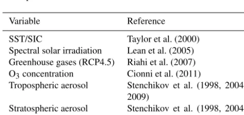
The ICON-ART simulation is configured as an AMIP (At-mospheric Model Intercomparison Project) like experiment (Gates et al., 1999). The boundary conditions used are sum-marised in Table 2. We set up two experiments on the R2B4
Figure 6.Daily snapshots at 00:00 UTC at 30 hPa of the passive vortex tracer in arbitrary units (upper left to bottom right). The pas-sive tracer was set to 1 within the vortex boundary at the beginning of the integration.
Table 2.Overview of the boundary conditions used in the AMIP-like experiments.
Variable Reference
SST/SIC Taylor et al. (2000)
Spectral solar irradiation Lean et al. (2005) Greenhouse gases (RCP4.5) Riahi et al. (2007) O3concentration Cionni et al. (2011)
Tropospheric aerosol Stenchikov et al. (1998, 2004, 2009)
Stratospheric aerosol Stenchikov et al. (1998, 2004, 2009)
(2011). This simulation is called “control”. The feedback simulation uses the interactive ozone as well as the addi-tional tendencies on water vapour, shown in Sect. 4.4. For all following diagnostics and discussions, the same two simula-tions are used. The results of the complete integration from 1979 to 2009 are found in Appendix B. In the following, analysis of the time span from 1990 to 2009 is shown. This avoids possible differences arising from changes in ozone de-pleting substances from 1979 to 1990 that are not considered in Linoz with time-invariant look-up tables.
Figure 7 shows the climatological ozone distribution at a pressure level of 50 hPa. Monthly averaged zonal means of ozone for the period of 1990 to 2009 are plotted twice. Fig-ure 7a shows the ozone used in the control run (ctrl) (Ta-ble 2). Figure 7b shows the modelled ozone of the non-interactive Linoz simulation, where modelled temperatures are the same as in the control run. Figure 7c shows the temporal evolution of the zonal mean ozone in the
feed-back simulation. Additionally, contour lines are represent-ing the interannual standard deviations of ozone in all pan-els. The black contour line represents a standard deviation of 1×10⁻⁷kg kg−1. Brighter colours present higher values of standard deviation with a spacing of 2×10⁻⁷kg kg−1.
A striking difference in the three ozone distributions shown in Fig. 7 is the duration of the ozone hole period in-dicated by the area that is shaded in dark blue. Modelled ozone (Fig. 7b, c) shows a much longer duration than the assumed background climatology. In addition, the duration of the ozone hole period increases slightly for the interac-tive integration. This is caused by the feedback of the mod-elled ozone, calculated with the Linoz parameterisation un-der consiun-deration of the correction term for a shorter ozone lifetime due to the presence of polar stratospheric clouds. From October to December, very low ozone concentrations of about 1×10⁻⁶kg kg−1can be seen in the panel for the non-interactive Linoz ozone (Fig. 7b). For the feedback sim-ulation, low ozone concentrations in the Southern Hemi-sphere, in conjunction with low temperatures, occur until the end of spring. The feedback process stabilises the Southern Hemisphere polar vortex, prolonging its lifetime by delay-ing the final warmdelay-ing. The default climatology of the ICON-ART control simulation does not represent very low values of ozone concentrations. This misrepresentation has also been discussed by, e.g. Arblaster et al. (2014). Here, the authors point out that most models that are using a prescribed ozone climatology tend to underestimate the Antarctic ozone de-pletion. Thus, modelled ozone values are higher than indi-cated by observations between 1979 and 2007 (e.g. Hassler et al., 2013). Taking the standard deviation into account, the characteristics of the AMIP ozone climatology (Cionni et al., 2011) become clearer. The contour lines represent a semicir-cle each winter in the Southern Hemisphere that is aligned with the ozone concentration gradients. This symmetric and coherent pattern of the ozone minimum is most likely not a very realistic representation of variability on top of an ozone hole that is not deep enough. The standard deviation iso-lines for the modelled ozone are different and intersect the isolines of ozone concentrations, with higher variabilities at later times in the ozone hole period.
We note that the standard deviations shown in Fig. 7 should be interpreted differently between the control and feedback simulations of ICON-ART. This is due to the fact that in the control simulation a time-varying background climatology is used that has an imposed long-term trend, whereas in the feedback simulation, no trend is imposed, and the internal variability of ICON-ART is the main component of the ozone variability. To illustrate this difference, we sum-marise the results of a time series decomposition in Table 3.
ICON-Jan May Sep Jan May Sep Mean month 90 60 30 0 30 60 90
Lat / degree
1e-07 1e-07 1e-07 1e-07 1e-07 1e-07 1e-07 1e-07 1e-07 3e-07 3e-07
(a) ICON-ART ctrl
Jan May Sep Jan May Sep
Mean month 1e-07 1e-07 1e-07 1e-07 3e-07 3e-07 3e-07 3e-07 3e-07 3e-07 5e-07 5e-07 7e-07
(b) ICON-ART ctrl Linoz
Jan May Sep Jan May Sep
Mean month 1e-07 1e-07 1e-07 1e-07 1e-07 1e-07 3e-07 3e-07 3e-07 3e-07 3e-07 3e-07 5e-07 5e-07 5e-07
5e-07 5e-07 5e-07
7e-07 7e-07
7e-07
7e-07 7e-07
(c) ICON-ART feedback
0.0e+00 2.0e-06 4.0e-06 6.0e-06 8.0e-06
Mean ozone at 50 hPa/ kg kg 1990–20091
Figure 7.Monthly averaged zonal means of ozone (kg kg−1) at 50 hPa (shown twice) for the period from 1990 to 2009 (shaded). Contour lines represent the standard deviation of the monthly means.(a)Ozone climatology as used in the control simulation;(b)non-interactive Linoz ozone;(c)interactive Linoz ozone.
ART simulations in two periods: 1980 to 1997 and 1997 to 2009. The ICON-ART control simulation shows an ozone de-cline for the earlier period and a small ozone increase for the later period (by construction of the background climatol-ogy). The feedback simulation shows no pronounced trend (as expected; see above) in particular during the later pe-riod. Note that the RMSE (root mean square error) is higher in both periods for the feedback simulation compared to the ICON-ART control simulation. The higher RMSE is induced by substantial year-to-year meteorological variability. Both model time series can be compared to the shorter TOMS on NIMBUS 7 time series (1997 to 2005).
5.3 Temperature changes due to ozone feedback
In the previous section, we have shown that with the change to an interactive representation of ozone the duration of the southern polar vortex is increased. Here, we provide more de-tails on the zonal mean temperature distributions in the con-trol and feedback simulations.
The direct impact of ozone, already mentioned in Sect. 5.2, is also displayed in the seasonal variation of the zonal mean temperatures; see Fig. 8.
In the Northern Hemisphere winter (DJF), temperatures of 210 K are reached between 100 and 10 hPa in the tropics. For the season of June–July–August (JJA), the temperature minimum in the tropics is at 100 hPa with temperatures as low as 200 K in both ICON-ART simulations. In the South-ern Hemisphere winter, ICON-ART control reaches temper-atures of about 200 K and ICON-ART feedback tempertemper-atures lower than 195 K. The Northern Hemisphere summer is rep-resented by temperatures higher than 260 K above 5 hPa.
Figure 9 shows the difference between control and feed-back runs. In the Southern Hemisphere winter, the effect described in Sect. 5.2 can be observed. Due to the lower polar vortex temperature, differences up to 5 K occur. The
1 5 10 50 100 500 1000
Pres / hPa
160 180 200 200 220 220 220 240 240 240 260 260 280 280
DJF (a) ICON-ART ctrl
1 5 10 50 100 500 1000
Pres / hPa
180 180 200 200 220 220 220 240 240 240 260 260 260 280 MAM 1 5 10 50 100 500 1000
Pres / hPa
160 180 200 200 200 220 220 240 240 240 260 260 260 280 280 300 JJA
90 60 30 0 30 60 90
Lat / degree 1 5 10 50 100 500 1000
Pres / hPa
195 195 195 210 210 210 225 225 225 240 240 240 255 255 255 270 270 285 285 SON 195 210 210 225 225 225 240 240 240 255 255 255 270 270285
DJF (b) ICON-ART feedback
195 210 210 210 225 225 225 240 240 240 255 255 255 270 270 270 285 MAM 200 200 220 220 240 240 240 260 260 260 280 280 300 JJA
90 60 30 0 30 60 90
Lat / degree 195 195 210 210 225 225 225 240 240 240 255 255 255 270 270 285 285 SON
150 180 210 240 270 300
Temperature / K 1990–2009
Figure 8. Latitude–height cross sections of seasonal and zonal mean temperature (K) for ICON-ART simulations from 1990 to 2009.(a)Control run;(b)feedback simulation.
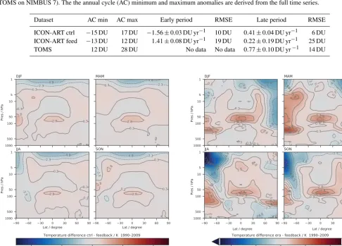
dif-Table 3.Results of the time series analysis for different time domains at 60◦S for the ozone total column. Results for both ICON-ART simulations and TOMS observation are shown. The early period is from 1980 to 1997 and the late period is from 1997 to 2009 (to 2005 for TOMS on NIMBUS 7). The the annual cycle (AC) minimum and maximum anomalies are derived from the full time series.
Dataset AC min AC max Early period RMSE Late period RMSE
ICON-ART ctrl −15 DU 17 DU −1.56±0.03 DU yr−1 10 DU 0.41±0.04 DU yr−1 6 DU ICON-ART feed −13 DU 12 DU 1.41±0.08 DU yr−1 19 DU 0.22±0.19 DU yr−1 25 DU
TOMS 12 DU 28 DU No data No data 0.77±0.10 DU yr−1 14 DU
1 5 10 50 100 500 1000
Pres / hPa
-25.0 -22.5
-22.5 -19.9 -17.4
-14.9 -12.4 -9.8 -7.3 -4.8 -2.3 0.3 0.3 0.3 0.3 2.8 2.8 DJF -25.0 -22.5 -19.9 -17.4 -14.9 -12.4 -9.8 -7.3 -4.8 -2.3 0.3 0.3 2.8 MAM
90 60 30 0 30 60 90
Lat / degree 1 5 10 50 100 500 1000
Pres / hPa
-25.0 -22.5 -19.9 -17.4 -14.9 -12.4 -9.8 -7.3 -4.8 -2.3 -2.3 0.3 0.3 0.3 0.3 2.8 JJA
90 60 30 0 30 60 90
Lat / degree -25.0
-22.5
-19.9
-17.4 -14.9 -12.4
-9.8 -7.3 -4.8 -2.3 -2.3 0.3 0.3 0.3 0.3 2.8 2.8 2.8 SON
-20.0 -10.0 0.0 10.0 20.0
Temperature difference ctrl - feedback / K 1990–2009
Figure 9. Latitude–height cross sections of seasonal and zonal mean temperature differences (K) for control minus feedback sim-ulation, as shown in Fig. 8.
ferent ozone distributions in the Southern Hemisphere win-ter. Within the tropical stratosphere, temperature differences of about 2.8 K can be seen. The differences of zonal and seasonal mean temperatures between ERA-Interim and the ICON-ART feedback simulation are shown in Fig. 10. The feature of a long-lasting Southern Hemisphere polar vortex is present as well, seen in high temperature differences of up to 20 K from September to November (SON). In general, the ICON-ART control simulation shows warmer temperatures than the ICON-ART feedback simulation, except for high al-titude ranges above 5 hPa.
The general structure is comparable to the results shown in the comparison studies of ECHAM5 (Roeckner et al., 2006). The difference between ERA-Interim and ICON-ART is in-creased in the Southern Hemisphere stratosphere. Neverthe-less, the representation of the polar vortex seems to be more realistic in the ICON-ART feedback simulation than in the control simulation. In the vertical region around 50 hPa, the
1 5 10 50 100 500 1000 -9.8 -7.3 -7.3 -4.8 -4.8 -4.8 -2.3 -2.3 0.3 0.3 0.3 0.3 0.3 0.3 0.3 0.3 0.3 2.8 2.8 2.8 5.3 5.3 5.3 7.8 7.8 DJF -12.4 -9.8 -7.3 -7.3 -4.8 -4.8 -4.8 -4.8 -2.3 -2.3 -2.3 -2.3 -2.3 -2.3 0.3 0.3 0.3 0.3 0.3 2.8 2.8 5.3 5.3 7.8 7.8 7.8 7.8 10.412.9 MAM
90 60 30 0 30 60 90
1 5 10 50 100 500 1000 -25.0 -22.5
-19.9-17.4-12.4-14.9
-9.8 -7.3 -4.8 -4.8 -4.8 -4.8 -2.3 -2.3 -2.3 -2.3 0.3 0.3 0.3 0.3 0.3 0.3 2.8 2.8 2.8 2.8 2.8 2.8 5.3 5.3 5.3 7.8 7.8 7.8 JJA
90 60 30 0 30 60 90
-17.4 -14.9 -12.4 -9.8 -7.3 -4.8 -4.8 -2.3 -2.3 -2.3 0.3 0.3 0.3 2.8 2.8 2.8 2.8 5.3 5.3 5.3 5.3 7.8 SON
-20.0 -10.0 0.0 10.0 20.0
Temperature difference era - feedback / K 1990–2009
Pres / hPa
Lat / degree
Pres / hPa
Lat / degree
Figure 10. Latitude–height cross sections of seasonal and zonal mean temperature differences (K) for ERA-Interim minus feedback simulation.
difference between ERA-Interim and the feedback simula-tion is about 15 to 20 K in the Southern Hemisphere and be-low 8 K in the tropics.
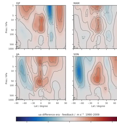
5.4 Zonal wind fields
Changes in temperature due to radiative feedback effects of ozone are also affecting the zonal wind structure. The zonal mean zonal wind is shown in Fig. 11. The left column shows the seasonal mean of the control ICON-ART simulation and the right column the feedback simulation. In both simula-tions, a strong eastward zonal wind with wind speeds up to 60 m s−1 is reached in the Southern Hemisphere winter (JJA). The wind speed patterns in the tropical stratosphere also match the seasonal mean analysis.
J. Schröter et al.: ICON-ART 2.1 4057 1 5 10 50 100 500 1000 -16.0 -8.0 -8.0 0.0 0.0 0.0 0.0 0.0
0.0 0.0 0.0
0.0 0.0 8.0 DJF -10.0 -5.0 -5.0 0.0 0.0 0.0
0.0 0.0 0.0 0.0
0.0 0.0
0.0 5.0 MAM
90 60 30 0 30 60 90
1 5 10 50 100 500 1000 -30.0 -20.0 -10.0 0.0 0.0 0.0 0.0 0.0 0.0 0.0 0.0 10.0 20.0 30.0 JJA
90 60 30 0 30 60 90
-10.0 -5.0 -5.0 0.0 0.0 0.0 0.0 0.0 0.0 0.0 0.0 0.0 0.0 5.0 10.0 15.0 20.0 SON
-40.0 -20.0 0.0 20.0 40.0
ua difference ctrl - feedback/ m s 1990–20091
Pres / hPa
Lat / degree
Pres / hPa
Lat / degree
Figure 11. Latitude–height cross sections of seasonal and zonal mean zonal wind differences (m s−1) for ICON-ART simulations from 1990 to 2009.
shows values up to 25 m s−1 lower than in the ICON-ART simulation. Between 30 and 60◦N latitude above 20 hPa, the sign of the differences changes. Here, we observe stronger zonal wind speeds than in ERA-Interim. The overall patterns are similar to the differences shown in Roeckner et al. (2006).
5.5 Water vapour
Here, we focus on the atmospheric water vapour tape recorder in ICON-ART. An atmospheric tape recorder can be defined as the vertical propagation of an anomaly that varies periodically in time with a tropospheric source (Gre-gory and West, 2002). The temporal and vertical distribution of the tropical stratospheric water vapour is a prominent ex-ample for an atmospheric tape recorder signal. The simulated stratospheric water vapour depends strongly on the tempera-tures that are encountered by an air parcel containing water vapour that is transported vertically from the troposphere up-wards toup-wards and through the tropopause (Schoeberl et al., 2012). The quantitative link between variations of tropical tropopause temperatures over decades and their influence on water vapour transfer into the stratosphere is still not fully understood (e.g. Rosenlof and Reid, 2008). It has been shown that stratospheric water vapour can have a strong impact on stratospheric climate (e.g. de F. Forster and Shine, 1999). Thus, the study of the water vapour tape recorder is an impor-tant tool for the further understanding of large-scale transport processes and climate change linkages.
1 5 10 50 100 500 1000
Pres / hPa
-24.0 -16.0 -8.0 -8.0 0.0 0.0 0.0 0.0 0.0 0.0 0.0 0.0 0.0 0.0 0.0 8.0 8.0 8.0 16.0 16.0 16.0 DJF -8.0 -4.0 -4.0 -4.0 0.0 0.0 0.0 0.0 0.0 4.0 4.0 8.0 8.0 12.0 12.0 16.0 16.0 20.0 MAM
90 60 30 0 30 60 90
Lat / degree 1 5 10 50 100 500 1000
Pres / hPa
-15.0 -10.0 -5.0 0.0 0.0 0.0 0.0 0.0 0.0 0.0 5.0 5.0 5.0 10.0 15.0 15.0 15.0 20.0 20.0 JJA
90 60 30 0 30 60 90
Lat / degree -24.0 -16.0 -8.0 0.0 0.0 0.0 0.0 0.0 0.0 0.0 0.0 8.0 8.0 8.0 16.0 16.0 SON
-40.0 -20.0 0.0 20.0 40.0
ua difference era - feedback / m s 1990–20091
Figure 12. Latitude–height cross sections of seasonal and zonal mean zonal wind differences (m s−1) for ERA-Interim minus feed-back simulation.
The tape recorder anomalies are calculated relative to the annual mean water vapour in the tropics (5◦N–5◦S). For this study, we use the water vapour tracer,qv. This tracer is the standard tracer of ICON itself. It is used in the radiation scheme and is not only transported but is also affected by the microphysical schemes. As in the previous section, ozone is calculated with the Linoz scheme and used interactively. The additional water tendencies by methane oxidation and pho-tolysis is also included in the stratospheric water budget.
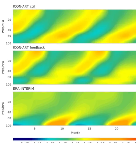
Figure 13 shows the stratospheric tape recorder. For the analysis, the years 1990 to 2009 are taken into account. We compare the ICON-ART results with the water vapour prod-uct from ERA-Interim. The calculated mean ERA-Interim tape recorder is shown in the bottom panel of Fig. 13.
The tape recorder signal for the ICON-ART control simulation shows lower values of anomalies down to
−7×10⁻⁷kg kg−1 in comparison to the feedback simula-tion (Fig. 13). For ERA-Interim, anomalies up to −2×
10−7kg kg−1 are diagnosed from February to June in the pressure range of 100 to 50 hPa.
20
40
60
100
Pres/hPa
ICON-ART ctrl
20
40
60
100
Pres/hPa
ICON-ART feedback
5 10 15 20
Month 20
40
60
100
Pres/hPa
ERA-INTERIM
-7e-07 -5e-07 -3e-07 -2e-07 -8e-09 2e-07 3e-07 5e-07 6e-07 8e-07 Mean monthly anomalies of water vapor / kg kg - 5° N–5° S1
Figure 13.Tropical (5◦N–5◦S) water vapour anomalies as monthly mean deviations (plotted twice) from the annual mean, averaged from 1990 to 2009, as a function of months and altitude.
the water vapour tape recorder is consistent with the results of the temperature differences, as seen in Fig. 9. Due to lower tropical tropopause temperatures in the feedback simulation, less water can enter the lower stratosphere. The annual mean temperature difference (not shown) shows that the control simulation is up to 2.8 K warmer than the feedback simula-tion between 100 and 50 hPa, in the tropics. The results corre-spond with the freeze-drying hypothesis explained above. In general, monthly mean anomalies are attenuated in the feed-back simulation compared to the simulation using the stan-dard ozone climatology, with in particular the winter months being more similar to ERA-Interim. Focusing on the strong positive anomaly between 100 and 50 hPa, from May to Au-gust, the explanation from above has to be extended. The an-nual mean shows a cold bias of the tropical tropopause. How-ever, referring to Fig. 9, one can see that, for that time span, the sign of temperature changes. In the feedback simulation, higher temperatures in the tropical tropopause are reached. Thus, more water vapour can enter the stratosphere which is a possible explanation for the strong positive anomaly.
The tape recorder signal of ERA-Interim shows a maxi-mum amplitude in the lower stratosphere between 100 and 60 hPa. In the ICON-ART control simulation, the lower stratospheric amplitude of the water vapour tape recorder is already smaller. With interactive ozone and water vapour, as in the ICON-ART feedback simulation, the lower strato-spheric amplitude is attenuated further. However, a relative maximum above 20 hPa occurs. This is likely the result of an overestimated water vapour tendency provided by the
methane oxidation, because methane is biased slightly high in the feedback simulation.
The slope of the latitude–height water vapour anomalies is nearly unchanged between non-interactive and interactive integrations. Thus, the velocity of the upward transport is largely unaffected by the inclusion of the radiative feedback. The result of both ICON-ART simulations in comparison to ERA-Interim is similar to the results presented in Jiang et al. (2015). Here, the authors combined measurements and sim-ulations of water vapour from the Microwave Limb Sounder (MLS), GMAO Modern-Era Retrospective Analysis for re-search and Applications in its newest version (MERRA-2) and ERA-Interim and used them for a comparison of the water vapour tape recorder behaviour. The upward transport above the tropical tropopause of ERA-Interim is found to be faster than the transport diagnosed from MLS measurements. Thus, in the current configuration, ICON-ART produces sim-ilar ascent rates to ERA-Interim, which are likely faster than observed.
We have shown that the change between interactive and non-interactive integrations with respect to tropical ascent rates is small. However, some changes are clearly de-tectable and the important relationship between the tropical tropopause minimum temperatures and water vapour concen-trations is qualitatively captured by the ICON-ART system. More comprehensive climate studies are in preparation.
5.6 Age of air
For the simulation of the age of air, we use the same setup as described in Sect. 5.3. As all other diagnostics, the age of air tracer is interpolated on a regular latitude–longitude grid with a horizontal resolution of 0.75◦×0.75◦on predefined
pressure levels.
The tracer is initialised as described in Sect. 4.3. The con-trol (ctrl) experiment is a simulation in which water vapour and ozone calculated within ICON-ART have no impact on the calculation of radiation. In the second experiment (feed-back), the altered ozone and water vapour distributions of ICON-ART are coupled to the radiation routine. The first 11 years of each simulation are excluded in the analysis to prevent spin-up effects contaminating the result.
1
5
50 100
500 1000
Pres / hPa
0.0 0.0
0.6 1.3
1.9 2.5
3.2
DJF (a) ICON-ART ctrl
1
5
50 100
500 1000
Pres / hPa
0.0 0.0
0.6
1.3
1.9 2.5
3.2
3.8
MAM
1
5
50 100
500 1000
Pres / hPa
0.0 0.0
0.6 1.3
1.9 2.5
3.2 3.8
3.8 JJA
90 60 30 0 30 60 90
Lat / degree 1
5
50 100
500 1000
Pres / hPa
0.0 0.0
0.61.3 1.9
2.5 3.2
3.8
3.8 SON
0.0 0.0
0.6
1.3 1.9
2.5 3.2
3.8
3.8
DJF (b) ICON-ART feedback
0.0 0.0
0.6 1.3 1.9
2.5 3.2 3.8 MAM
0.0 0.0
0.6 1.3
1.9
2.5 3.2
3.8 JJA
90 60 30 0 30 60 90
Lat / degree
0.0 0.0
0.6 1.3
1.9
2.5 3.2
3.8 SON
0.0 1.5 3.0 4.5 6.0
Age of air/ yr 1990–2009
Figure 14. Latitude–height cross sections of seasonal and zonal mean ages of air (year) for ICON-ART simulations from 1990 to 2009.(a)Control run;(b)feedback simulation.
Jan May Sep Jan May Sep
Mean month 90
60 30 0 30 60 90
Lat
0.10
0.10
0.10 0.10
0.20
0.20
0.20 0.20 0.20
(a) ICON ctrl
Jan May Sep Jan May Sep
Mean month 0.10
0.10
0.10
0.10
0.20 0.20 0.20
0.20 (b) ICON feedback0.20 0.20
0 1 2 3 4 5
Age of air at 50 hPa/ years 1990–2009
Figure 15. Monthly averaged zonal means of age of air (year) at 50 hPa (shown twice) for the period from 1990 to 2009 (shaded). Contour lines represent the standard deviation of the monthly means.(a)Control run;(b)feedback simulation.
of ozone and water vapour on radiation and thus on transport processes. The age of air in the feedback simulation is up to 6 months older than the control simulation. Figure 15 shows the climatological mean age of air, in the same representa-tion as shown in Fig. 7. Here, the temporal and zonal means
of the age of air from 1990 to 2009 are taken at an altitude of 50 hPa. The standard deviation from the mean is represented by the contour lines. These lines represent the interannual variability. The absolute mean age of air is higher for the feedback simulation on both hemispheres. The band of low values in the tropics is narrowed for the feedback simulation. The values of standard deviation are comparable. However, in the region of the Southern Hemisphere polar vortex, from October to January, the standard deviation is higher for the feedback than for the control simulation. Since the polar vor-tex is stabilised by the ozone feedback, a different dynamical situation can be observed, influencing the interannual vari-ability of the age of air. In comparison to other studies, which focus on other time spans (e.g. Brasseur and Solomon, 2006; Engel et al., 2009; Stiller et al., 2012; Haenel et al., 2015), ICON-ART shows an age of air which is too young compared to observations. But this behaviour has also been observed in other studies with different models, as described in, e.g. Monge-Sanz et al. (2007) or Hoppe et al. (2014). With this diagnostic, the general representation of stratospheric trans-port processes can be investigated further.
6 Conclusions
We present a new flexible tracer framework developed for ICON-ART. The next-generation model ICON-ART can be used for many different applications currently ranging from forecasting to climate simulations. ICON is used for LES simulations, operationally for numerical weather forecasting and for climate simulations. All three application areas have very different demands in terms of model configurations, in-cluding the set of tracers and tracer interactions to be sim-ulated. For future studies using ICON-ART, a fast adaption of the selected tracers and interactions to the experimental requirements is of high importance. With our new flexible tracer framework, tracers can be added and configured with-out any changes to the model source code. This allows users to easily perform complex model experiments. In a forward-thinking manner, we also provide the option to extend the existing tracer structure and submodule awareness of tracer subsets. Within the scope of the paper, we demonstrate the tracer framework and its applicability for a range of simu-lations. We present one hindcast case study and AMIP-type climate integrations.