JIEMS
Journal of Industrial Engineering and Management Studies Vol. 3, No. 2, pp. 88-106
www.jiems.icms.ac.ir
Designing a New Multi-objective Model for a Forward/Reverse
Logistic Network Considering Customer Responsiveness and
Quality Level
A.Yaghoubi1,*, M. Asghari2
Abstract
In today’s competitive world, the need to supply chain management (SCM) is more than ever. Since the purpose of logistic problems is minimizing the costs of organization to create favorable time and place for the products, SCM seek to create competitive advantage for their organizations and increase their productivity. This paper proposes a new multi-objective model for integrated forward / reverse logistics network including three objective functions which belongs to the class of NP-hard problems. The first objective attempts to minimize the total cost of the supply chain network. The second objective attempts to maximize the customer service level (customer responsiveness) in both forward and reverse networks. The third objective tries to minimize the total number of defects of in raw material obtained from suppliers and thus increase the quality level. To solve the proposed model, the non-dominated sorting genetic algorithm (NSGA-II) and non-dominated ranked genetic algorithms (NRGA) are used. A Taguchi experimental design method was applied to set and estimate the proper values of GAs parameters for improving their performances. Besides, to evaluate the performance of the two algorithms some numerical examples are produced and analyzed with some metrics to determine which algorithm works better. In order to determine whether there is a significant difference between the performances of the algorithms, the one-way ANOVA and Tukey test are used at 0.95 confidence level. Finally, the performance of the algorithms is analyzed and the results are reported.
Keywords: Supply Chain Management, Logistic Network, Non-Dominated Sorting Genetic Algorithm (NSGA-II), Non-dominated Ranked Genetic Algorithms (NRGA).
1. Introduction
A Supply chain network design problem involves the sum of facilities organized to gain and transfer raw materials to finished products, distribute these products and present the services after selling to fulfill the customer needs. This problem determines the number, location, capacity level and technology of the facilities to be considered.
*Corresponding Author;[email protected]
1Department of Industrial Engineering, Raja Higher Education Institute, Qazvin, Iran.
An effective, efficient and robust logistics network becomes a sustainable competitive advantage for firms and helps them to cope with increasing environmental turbulence and more intense competitive pressures. In most of the past researches the design of forward and reverse logistics networks is considered separately, but the configuration of the reverse logistics network has a strong influence on the forward logistics network and vice versa. Separating the design may result in sub-optimality, therefore the design of the forward and reverse logistics network should be integrated (Ramezani et al, 2013). Due to the fact that designing the forward and reverse logistics separately leads to sub-optimal designs with respect to costs, service levels and responsiveness, the design of the forward and reverse logistics networks should be integrated.
This kind of integration can be considered as “horizontal integration’’, as it encompasses the integration of related optimization problems at the same decision level (Jacobs and Chase, 2008). Based on the considerations described above, this study presents a new mixed integer programming model for integrated forward / reverse logistics network including four objective functions: total profit, transportation costs, system service and total pollution generated for transferring products with considering customer responsiveness and quality level as objectives of the logistic network. The rest structure of this paper is as follows. Section 2 provides a systematic literature review for the forward/reverse logistic network design. In Section 3, we present a new multi-objective model for integrated forward / reverse logistics network including three objective functions. In section 4, the applications of two meta-heuristic algorithms including NSGA-II and NRGA are described to solve the proposed model. Section 5 is devoted to the computational experiments and the analysis of the results. Finally, some conclusions and suggestions are presented in Section 6.
2. Literature Review
Previous research in the area of forward/ reverse and integrated logistics network design often limited itself to single-objective (minimizing the cost or maximizing the profit) in front logistic. But, real world network design problems are often characterized by multiple objectives. The minimization of total costs and maximization of network responsiveness are the most commonly used single objectives in the forward logistics network design. These objectives are, however, typically conflicting, and considering them concurrently is the most favorable option for most decision makers. Network responsiveness is an important issue in reverse logistics too, as it is undesirable for customers/retailers to keep used products for a long time because of the related holding costs.
Franca et al (2009) presented a stochastic multi-objective model for a forward logistic network that uses the Six Sigma measure to evaluate the quality of raw materials acquired by suppliers. The objectives of the problem are to maximize the profit of SC and minimize the total number of defective raw material parts under demand uncertainty. A bi-objective integrated forward/reverse supply chain design model was suggested by Pishvaee et al (2010), in which the costs and the responsiveness of a logistic network are considered as objectives of the model. They developed an efficient multi-objective memetic algorithm by applying three different local searches in order to find the set of non-dominated solutions. El-Sayed et al (2010) presented a multi-period multi-echelon forward/reverse logistic network design model while the objective of their model is to maximize the profit of a supply chain. The suggested network structure include the three direct path level (suppliers, facilities centers and gathering) and two
In the context of reverse logistics various models have been developed in the last decade. Krikke et al. (2003) designed a MILP model for a two-stage reverse supply chain network for a copier manufacturer. In this model processing costs of returned products and inventory costs are noticed in the objective function for minimizing the total cost. Pishvaee et al (2010) analyzed the cost of logistic network in multi-period with combinational genetic algorithm. Rajagopal (2015) reviewed and identified the types of logistics and compared the Reverse Logistics with Forward Logistics for better understanding and gaining competitive advantages. Giri & Sharma (2015) develop algorithms for sequential and global optimization to study the closed-loop supply chain comprised of the raw material supplier, manufacturer, retailer, and collector. They account for product quality by determining a level of quality above which items are sent to remanufacturing, and they report good results of their proposed algorithms. Anne et al. (2016) explained about reverse logistics and the influence of competitiveness among the food processing industries in Kenya. They proposed a framework for reverse logistics practices.
From the analysis, they found that there is a positive relationship between reverse logistics and proper utilization of material and also reduces cost and enhance competitiveness of the firm. Binti et al. (2016) demonstrated the reverse logistics in the food and beverage industries in Malaysia. They have formed the framework based on five dimensions and collected the feedback. From that the feedback they highlight the present scenario and investigated the internal and external barriers of the industries. Yadegari et al. (2017) presented an integrated forward/reverse logistics model, while considering three kinds of transportation modes. They proposed a memetic algorithm to solve the model.
Table 1. Network type code
Category Detail
Code
Network Types Forward Logistic
FL
Reverse Logistic RL
Forward/Reverse Logistic FR
Network Layers Production Centers
MC
Distribution Centers DC
Collection Centers CC
Reproduction Centers RMC
Recycling centers RYC
Disposal centers DSC
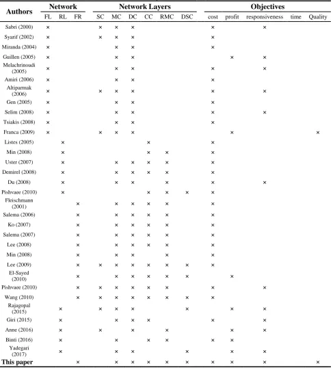
Table 2. A summary of the review literature
Authors Network NetworkLayers Objectives
FL RL FR SC MC DC CC RMC DSC cost profit responsiveness time Quality
Sabri (2000) × × × × × ×
Syarif (2002) × × × × ×
Miranda (2004) × × × ×
Guillen (2005) × × × × ×
Melachrinoudi
(2005) × × × × ×
Amiri (2006) × × × ×
Altiparmak
(2006) × × × × × ×
Gen (2005) × × × ×
Selim (2008) × × × × ×
Tsiakis (2008) × × × ×
Franca (2009) × × × × × ×
Listes (2005) × × ×
Min (2008) × × × ×
Uster (2007) × × × × × ×
Demirel (2008) × × × × × ×
Du (2008) × × × × × ×
Pishvaee (2010) × × × × ×
Fleischmann
(2001) × × × × × ×
Salema (2006) × × × × × ×
Ko (2007) × × × × × ×
Salema (2007) × × × × × ×
Lee (2008) × × × × × ×
Min (2008) × × × × ×
Lee (2009) × × × × × × × ×
El-Sayed
(2010) × × × × × × ×
Pishvaee (2010) × × × × × × × ×
Wang (2010) × × × × × × × ×
Rajagopal
(2015) × × × × × × ×
Giri (2015) × × × × × ×
Anne (2016) × × × × × ×
Binti (2016) × × × × × ×
Yadegari
(2017) × × × × × ×
Contribution: Although a number of researches are performed in SCND problem, but to the best of knowledge, there is no study that addresses the issues of chain profit, supplier quality and customer responsiveness in context of a Forward/Reverse Logistic. Table 2 shows the distinctiveness of this paper from others in the literature.
3. Problem Description
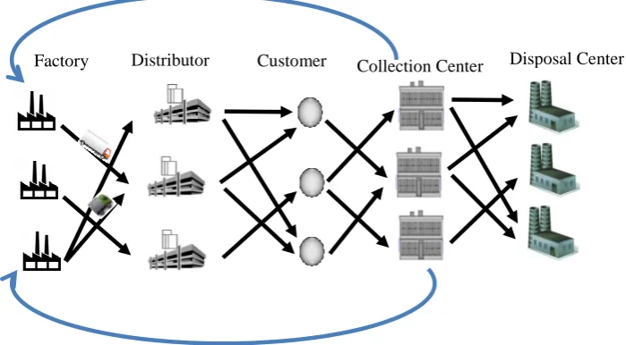
The integrated logistics network (ILN) discussed in this paper including supply centers or factories, distributers, customer zones, collection centers and disposal centers with multi-level capacities. The general structure of the proposed closed-loop logistic network is illustrated in Fig. 1.
- In forward direction, the factories are responsible for providing the products to customers. The products are conveyed from factories to customers via distribution centers to meet the customer demands.
- In the reverse direction, returned products are collected in collection centers and, after testing, the recoverable products are shipped to factories, and scrapped products are moved to disposal centers. By means of this strategy, excessive transportation of returned products is prevented and the returned products can be moved directly to the factories.
Figure 1. An integrated forward/reverse logistics network
In the forward network, products are pulled through a divergent network and in the reverse network, returned products are moved through a semi-convergent network according to push principles. A predefined percentage of demand from each customer zone is assumed to result in returned products and a predefined value is determined as an average disposal rate. The recovery process is performed in recovery centers and recovered products are inserted in the forward network and are considered identical to new products. Thus, the integrated forward/reverse logistics network is a closed-loop logistics network. It is important to note that the design of the integrated logistics network may involve a trade-off between the total costs and the network’s responsiveness. In some cases, factories may decide to open more facilities to increase the responsiveness for higher customer satisfaction, which may lead to a greater
investment cost. Thus, the integrated forward/reverse logistics network is designed to jointly take network costs and network responsiveness into account.
1.1. Model Assumption
Supply chain network includes three fronting level (supplier or factories, customers and distribution centers) and two levels in backing part (collection centers, disposal center). The model is designed for one period.
All return products are provided from demand market in collection centers. The demand value of customers are specified.
Factory locations and capacity, distribution centers, processing and disposal are specified.
Customer situations are fixed and specified.
The flow is only permitted to be transported between two consecutive stages. Moreover, there are no flows between facilities at the same stage.
The quantity of price, production costs, operating costs, collection costs, disposal costs, demands and return rates are fixed and specified.
The proposed model consists of three objective functions. The first objective attempts to minimize the total cost of the supply chain network. The second objective attempts to maximize the customer service level (customer responsiveness) in both forward and reverse networks. The third objective tries to minimize the total number of defects of in raw material obtained from suppliers and thus increase the quality level.
1.2. Problem Parameters
i Index of distributor type i, (i=1,…,m)
j Index of customer type j, (j=1,…,n) v Index of vehicle type v, (v=1,...,V)
p Index of product type p, (p=1,…,P)
Ni Set of possible levels for making a distributor in Group i
l Index of collection center type l, (l=1,…,L)
k Index of quality level type k, (k=1,…,K)
s Index of disposal center type s, (s=1,…,S)
capinp Capacity of distributor i for product type p with capacity level n
qpv Capacity of vehicle v for product type p
demandjp Demand of customer j for product type p
costin Making Cost of distributor type i with capacity level n
c1p,k Production cost of product type p with using useful materials for the environment with quality type k
c2s,k Product processing cost on disposal center s with using clean technology with quality level k
co1v The amount of product pollution by carriers v per unit
co2p,k The amount of pollution produced of the product type p by manufacturer p with quality level k
co3s,k The amount of pollution produced of the product type p by disposal center s with quality level k
slp,k The ratio of return redistribution average of p-type products are made with quality level k
sip,k The ratio of disposal average of p-type products are made with quality level k
rep,j,l The amount of product type p that is returned by customer type j to collection center l
prod p The amount of production of product type p
di,j The distance between distributer i and j node
di,p′ The distance between distributer i and location of product type p
dj,l The distance between customer j and collection center type l
cv Operational cost of vehicle v per unit
sep,k Selling price of product type p (per unit) with quality level k
1.3. Problem Variables
Xi,j,vp A binary variable that indicates the distributer i located before node j in the path of
vehicle v which carrier product type p
Yin A binary variable that indicates in the location of node i, a distributor with capacity level n be created
Zi,jp A binary variable that indicates customer j get product type p from distributer i
Hi,vp A binary variable that indicates the product type p transferred to distributer i by vehicle v
Mp,k A binary variable that indicates the manufacture of product type p uses useful material at quality level k
Ns,k A binary variable that indicates the disposal center s uses clean technology at level k to disposal product
Sp,j,l A binary variable that indicates the returned product type p from customer j be
transferred to collection center l
Tp,l,s A binary variable that indicates the collected product type p from collection center l be
transferred to disposal center s
Wi,vp A Slack variable relating to sub tour elimination constraint
In terms of the above notation, the mixed integer multi-objective model for a forward/reverse logistic network with considering customer responsiveness and quality level can be formulated
min 𝑂𝐹1 = ∑ ∑ ∑ 𝐻𝑖,𝑣𝑝 × 𝑐𝑣 × 𝑑𝑖,𝑝′ 𝑝∈𝑃
𝑣∈𝑉 𝑖∈𝐼
+ ∑ ∑ ∑ ∑ 𝑋𝑖,𝑗,𝑣𝑝 × 𝑐𝑣× 𝑑𝑖,𝑗
𝑝∈𝑃 𝑣∈𝑉 𝑗∈(𝐼∪𝐽) 𝑖∈(𝐼∪𝐽)
+ ∑ ∑ ∑ 𝑟𝑒𝑝,𝑗,𝑙× 𝑑𝑗,𝑙
𝑙∈𝐿 𝑗∈𝐽 𝑝∈𝑃
+ ∑ ∑ 𝑌𝑖𝑛𝐶𝑂𝑆𝑇
𝑖𝑛
𝑖∈𝐼
𝑛∈𝑁𝑖
+ ∑ ∑ 𝑝𝑟𝑜𝑑 𝑝 𝑘∈𝐾
× 𝑀𝑝,𝑘
𝑝∈𝑃
× 𝑐1𝑝,𝑘
+ ∑ ∑ ∑ ∑ ∑ 𝑟𝑒𝑝,𝑗,𝑙 × 𝑠𝑖𝑝,𝑘× 𝑇𝑝,𝑙,𝑠 × 𝑁𝑠,𝑘
𝑠∈𝑆 𝑗∈𝐽 𝑙∈𝐿 𝑘∈𝐾 𝑝∈𝑃
× 𝑐2𝑠,𝑘
(1)
max 𝑂𝐹2 = ∑ ∑ ∑ 𝑍𝑖,𝑗𝑝
𝑝∈𝑃 𝑗∈𝐽 𝑖∈𝐼
× 𝑑𝑒𝑚𝑎𝑛𝑑𝑗𝑝 (2)
min 𝑂𝐹3 = ∑ ∑ ∑ 𝐻𝑖,𝑣𝑝 𝑑𝑖,𝑝′ 𝑐𝑜1𝑣 𝑝∈𝑃
𝑣∈𝑉 𝑖∈𝐼
+ ∑ ∑ 𝑝𝑟𝑜𝑑 𝑝 𝑘∈𝐾
× 𝑀𝑝,𝑘× 𝑐𝑜2𝑝,𝑘
𝑝∈𝑃
+ ∑ ∑ ∑ ∑ ∑ 𝑟𝑒𝑝,𝑗,𝑙 × 𝑠𝑖𝑝,𝑘× 𝑇𝑝,𝑙,𝑠 × 𝑁𝑠,𝑘
𝑠∈𝑆 𝑗∈𝐽 𝑙∈𝐿 𝑘∈𝐾 𝑝∈𝑃
× 𝑐𝑜3𝑠,𝑘
(3)
Subject to:
∑ 𝑋𝑖,𝑗,𝑣𝑝
𝑖∈(𝐼∪𝐽)
− ∑ 𝑋𝑗,𝑖,𝑣𝑝
𝑖∈(𝐼∪𝐽)
= 0 ∀𝑗 ∈ 𝐼 ∪ 𝐽, 𝑣 ∈ 𝑉, 𝑝 ∈ 𝑃 (4)
∑ 𝐻𝑖,𝑣𝑝 × 𝑞𝑣𝑝
𝑣∈𝑉
≤ ∑ 𝑐𝑎𝑝𝑖𝑛𝑝× 𝑌𝑖𝑛
𝑛∈𝑁𝑖
∀𝑖 ∈ 𝐼, 𝑝 ∈ 𝑃 (5)
∑ ∑ 𝑋𝑖,𝑗,𝑣𝑝
𝑗∈𝐽 𝑖∈(𝐼∪𝐽)
× 𝑑𝑒𝑚𝑎𝑛𝑑𝑗𝑝 ≤ 𝑞𝑣𝑝 ∀𝑣 ∈ 𝑉, 𝑝 ∈ 𝑃 (6)
∑ 𝑍𝑖,𝑗𝑝
𝑗∈𝐽
× 𝑑𝑒𝑚𝑎𝑛𝑑𝑗𝑝 ≤ ∑ 𝐻𝑖,𝑣𝑝 × 𝑞𝑣𝑝
𝑣∈𝑉 ∀𝑖 ∈ 𝐼, 𝑝 ∈ 𝑃
(7)
∑ 𝑋𝑖,𝑢,𝑣𝑝 + ∑ 𝑋𝑢,𝑗,𝑣𝑝 − 𝑍𝑖,𝑗𝑝 ≤ 1
𝑢∈(𝐼∪𝐽)
𝑢∈(𝐼∪𝐽) ∀𝑖 ∈ 𝐼, 𝑗 ∈ 𝐽, 𝑣 ∈ 𝑉, 𝑝 ∈ 𝑃
(8)
∑ ∑ 𝑌𝑖𝑛𝑐𝑜𝑠𝑡𝑖𝑛
𝑖∈𝐼
𝑛∈𝑁𝑖
≤ 𝑏𝑢𝑑𝑔𝑒𝑡 (9)
∑ ∑ 𝐻𝑖,𝑣𝑝 × 𝑞𝑣𝑝 ≤
𝑣∈𝑉 𝑖∈𝐼
𝑝𝑟𝑜𝑑 𝑝
∀ 𝑝 ∈ 𝑃 (10)
𝑟𝑒𝑝,𝑗,𝑙 = ∑ ∑ 𝑍𝑖,𝑗𝑝
𝑘∈𝐾 𝑖∈𝐼
× 𝑆𝑝,𝑗,𝑙× 𝑑𝑒𝑚𝑎𝑛𝑑𝑗𝑝
× 𝑠𝑙𝑝,𝑘× 𝑀𝑝,𝑘
∑ ∑ 𝑋𝑖,𝑗,𝑣𝑝
𝑣∈𝑉 𝑖∈(𝐼∪𝐽)
≤ 1 ∀𝑗 ∈ 𝐽, 𝑝 ∈ 𝑃 (12)
∑ 𝑌𝑖𝑛 ≤ 1
𝑛∈𝑁𝑖
∀𝑖 ∈ 𝐼 (13)
∑ 𝑍𝑖,𝑗𝑝 ≤ 1
𝑖∈𝐼
∀ 𝑗 ∈ 𝐽, 𝑝 ∈ 𝑃 (14)
∑ 𝐻𝑖,𝑣𝑝 ≤ 1
𝑣∈𝑉
∀ 𝑖 ∈ 𝐼, 𝑝 ∈ 𝑃 (15)
∑ 𝑀𝑝,𝑘≥ 𝑍𝑖,𝑗𝑝 𝑘∈𝐾
∀ 𝑖 ∈ 𝐼, 𝑗 ∈ 𝐽, 𝑝 ∈ 𝑃 (16)
∑ 𝑁𝑠,𝑘 ≥ 𝑇𝑝,𝑙,𝑠
𝑘∈𝐾
∀ 𝑝 ∈ 𝑃, 𝑙 ∈ 𝐿, 𝑠 ∈ 𝑆 (17)
∑ 𝑇𝑝,𝑙,𝑠
𝑠∈𝑆
≥ ∑ 𝑆𝑝,𝑗,𝑙
𝑗∈𝐽 ∀ 𝑝 ∈ 𝑃, 𝑙 ∈ 𝐿
(18)
𝑊𝑖,𝑣𝑝 − 𝑊𝑗,𝑣𝑝 + 𝑁𝑋𝑖,𝑗,𝑣𝑝 ≤ 𝑁 − 1 ∀𝑖, 𝑗 ∈ 𝐽, 𝑣 ∈ 𝑉, 𝑝 ∈ 𝑃 (19)
𝑋𝑖,𝑗,𝑣𝑝 , 𝑌𝑖𝑛, 𝑍𝑖,𝑗𝑝 , 𝐻𝑖,𝑣𝑝 , 𝑆𝑝,𝑗,𝑙, 𝑀𝑝,𝑘, 𝑁𝑠,𝑘,
𝑇𝑝,𝑙,𝑠 ∈ {0, 1} ∀𝑖, 𝑗, 𝑝, 𝑣, 𝑛, 𝑙, 𝑘, 𝑠 (20)
The first objective function (1) attempts to minimize the total cost of the supply chain network including: supply cost for purchasing the raw materials from factories, fixed cost for establishing the facilities, production cost for manufacturing the products in factories, inspection cost for the returned products in collection centers, operating cost in distribution centers, remanufacturing cost for recoverable products in factories and disposal costs for scrapped products. The second objective function (2) attempts to maximize the customer service level (customer responsiveness) in both forward and reverse networks. The third objective function (3) tries to minimize the total number of defects of in raw material obtained from factories and thus increase the quality level.
Constraint (4) insures that, for each product, the flow entering to each distribution center is equal to the flow exiting from this distribution center over each vehicle. Constraint (5) shows that the sum of the flow exiting from each distribution centers to all customers does not exceed the capacity of relevant vehicle. Constraint (6) shows that the sum of the flow entering to all customers by each vehicle does not exceed the capacity of relevant vehicle. Constraint (7) represents that the sum of the flow entering to each customer by various vehicles does not exceed the capacity of relevant vehicles. Constraint (8) shows the relation between allocation and routing in a model. Customer j allocates to the distributor i just if the vehicle v passes from customer j location, so it starts its journey from distributor i. Constraint (9) sets control the total budget. Constraint (10) ensures that the sum of the product type p which can moved by vehicle v does not exceed the capacity of production of it. Constraint (11) sets the returned products from customers to each collection center.
ensures that at least one of the products received by the customer from distributers, Must be produced with quality level type k.
Constraint (17) ensures that at least one of the collected products transferred to each disposal center from collection centers, Must be used with clean technology at level type k. Constraint (18) represents that if a product enters to a collection center, one disposal center should be allocated till returning the entering products to elimination center. Constraint (19) prevents the creation tour. Constraints (20) impose the binary restriction on the corresponding decision variables.
As the integrated forward/reverse logistics network design problem includes the capacitated plant location problem which is known to be NP-complete (Davis and Ray, 1969), the proposed model design problem is NP-hard. So, the performance of the proposed model is compared with two well-known multi-objective evolutionary Algorithms, namely NSGA-II and NRGA.
1.4.NSGA-II
Non–dominated sorting genetic algorithm II (NSGA-II) is one of the most well-known and efficient multi-objective evolutionary algorithms introduced by Deb et al. (2002). Ranking and selecting the population fronts are performed by non-dominance technique and a crowding distance. Also, the algorithm uses crossover and mutation operators to generate offspring are combined together. Finally, the best solution
in terms of non-dominance and crowding distance is selected from combined population as the new population. The non-dominated technique, the calculation of crowding distance, and crowding selection
operator will be explained as follows.
Assume that there are r objective functions. When the following conditions are satisfied, the solution X1 dominates solution X2. If X1 and X2 do not dominate each other, they are placed at the same front. For all objective functions, solution X1 is not worse than another solution X2. For at least one of the r objective functions X1 is really better than X2. Front number 1 is made by all solutions that are not dominated by any other solutions. Also front number 2 is built by all solutions that are only dominated by solutions in front number 1.
4. 1. 1. Crowding Distance
The crowding distance is a measure for density of solutions. The value of the crowding distance presents an estimate of density of solutions surrounding a particular solution. The solutions having a lower value of the crowding distance are preferred over solutions with a higher value of crowding distance.
4. 1. 2. Tournament Selection Operator
A binary tournament selection procedure has been applied for selecting solution for both the crossover and mutation operators. At first, select two solutions among the population size, then the lowest front number is selected if the two populations are from different fronts. If they become from the same front, the solution with the highest crowding distance is selected.
1.5. NRGA
tiers ranked based roulette wheel selection are used (one tier to select the front and the other to select solution from the front).
The front probability obtained as Eq. (21).
2* , 1,...,
*( 1)
i
i F
F F
rank
P i N
N N
Where NF show the number of fronts. In this equation, it is obvious that a front with highest
rank has the highest probability to be selected. So the probability of individuals fronts based on their crowding distance criteria is calculated as follows:
2* , 1,..., , 1,...,
*( 1)
ij
ij F i
i i
rank
P i N j M
M M
Where Mi show the number of individuals in the front i. In this equation individuals with more
crowding distance have more selection probability. The diversity among non-dominated solutions is also considered. Next, roulette wheel selection is applied according to the two random numbers (indicate number of front and individual chromosome in selected front) in intervals [0, 1] and [0, 1] respectively. This process is repeated until the desired number of individuals has been selected.
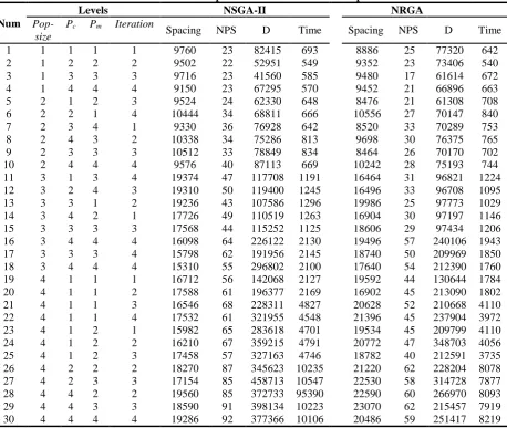
5. Test problems
In order to assess the performance of the proposed model, a summary of experiments is provided in this section. Some authors mentioned that increasing the amount of model’s parameters significantly increases the computational time with limited benefit in solution accuracy (Ramezani et al, 2013). Our experiments on the proposed model also confirm this judgment. Here to assess the performance of the proposed model, 30 test problems are selected which used 6 types of products. For each type, 5 test problems were designed which including various numbers of factory, distributers center, customer, collection location and disposal center. Test problems are solved with Matlab R2010b software on a Pentium dual-core 2.2 GHz computer with 2 GB RAM.
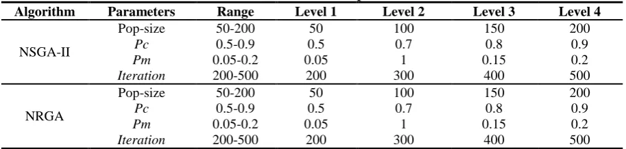
5.1. Parameter Tuning
Since the results of all meta-heuristics techniques are sensitive to their parameter setting, it is required to do extensive simulations to find suitable values for various parameters. The parameters of the NSGA-II and NRGA are pop-size, Pc, Pm and iteration (Al jadaan et al., 2008). The parameters of the two meta-heuristics algorithm are regulated using a Taguchi approach. In this approach, in the first stage, an L25 (55)orthogonal array experiment was
arranged under Taguchi parameter standard setting values, in which no. 1 to no. 25 were Taguchi experimental data. Accordingly, the control factor’s range was given four levels, as depicted in Table 3. For the second stage, it is similar to that of the first stage. An L25 (55)
orthogonal array experiment was also utilized to perform the process. The multiple quality characteristics and energy efficiency are the performance of injection molding process. Accordingly, the control factor’s range was given four levels, as depicted in Table 3. Overall, the range of factors in Table 3 covered the optima parameters under simulation (Maosheng et al., 2016). To achieve this aim using Taguchi, we carried out extensive experiments to determine effective parameters.In order to execute the procedure, we used MINITAB software
(21)
for finding the relation between responses (objective functions) and effective factors on responses (pop-size, Pc, Pm and iteration) that results are presented in Table 3.
Table 3. NSGA-II and NRGA parameter sets
Algorithm Parameters Range Level 1 Level 2 Level 3 Level 4
NSGA-II
Pop-size 50-200 50 100 150 200
Pc 0.5-0.9 0.5 0.7 0.8 0.9
Pm 0.05-0.2 0.05 1 0.15 0.2
Iteration 200-500 200 300 400 500
NRGA
Pop-size 50-200 50 100 150 200
Pc 0.5-0.9 0.5 0.7 0.8 0.9
Pm 0.05-0.2 0.05 1 0.15 0.2
Iteration 200-500 200 300 400 500
5.2. Comparison Metrics
Due to the conflicting nature of Pareto curves, we should use some performance measures to have a better assessment of multi-objective algorithms. So the following four performance metrics are considered (Tavakkoli-Moghaddam et al. 2011):
5.2.1. Number of Pareto Solution
The number of Pareto solution (NPS), which shows the number of Pareto optimal solutions that each algorithm can find.
5.2.2. Spacing Metric
We define the spacing (SM) metric by:
1
1
( 1)
n
i i
d d
SM
n d
where di is the Euclidean distance between consecutive solutions in the obtained non-dominated
set of solutions and d is the average of these distances. This metric provides an ability to measure the uniformity of the spread of the solution set points. Due to the discontinuous test problem, the trade-off surface of these problems has some holes and leads to difficulty in interpreting this metric. Our approach with this metric is identical to the number of non-dominated solutions on using the ANOVA method, except that the effects are investigated on the spacing metric.
5.2.3. Diversification Metric
Diversification metric (DM) measures the spread of the solution set and is defined as:
1
max( )
N
i i
t t
i
DM x y
Where xti yti is the Euclidean distance between non-dominated solution xti and
non-dominate i t
y .
5.2.4. Computational Time
The fourth metric is computational time of the algorithm (CPU) which indicates the computational time of each meta-heuristic algorithm.
(23)
Table 4. Results of the experiment of different size test problems NRGA NSGA-II Levels Num Time D NPS Spacing Time D NPS Spacing Iteration Pm Pc Pop-size 642 77320 25 8886 693 82415 23 9760 1 1 1 1 1 540 73406 23 9352 549 52951 22 9502 2 2 2 1 2 672 61614 17 9480 585 41560 23 9716 3 3 3 1 3 663 66896 21 9452 570 67295 23 9150 4 4 4 1 4 708 61308 21 8476 648 62330 24 9524 3 2 1 2 5 840 70147 27 10556 666 68811 34 10444 4 1 2 2 6 753 70289 33 8520 642 76928 36 9330 1 4 3 2 7 765 76375 30 9698 813 75286 34 10338 2 3 4 2 8 702 70170 26 8464 834 78849 33 10512 3 3 3 2 9 744 75193 28 10242 669 87113 40 9576 4 4 4 2 10 1224 96821 31 16464 1191 117708 47 19374 4 3 1 3 11 1095 96708 33 16496 1245 119400 50 19310 3 4 2 3 12 1029 97773 25 19986 1296 107586 43 19236 2 1 3 3 13 1146 97197 30 16904 1263 110519 49 17726 1 2 4 3 14 1206 97434 29 18606 1125 115252 44 17568 3 3 3 3 15 1943 240106 57 19496 2130 226122 64 16098 4 4 4 3 16 1850 209969 50 18740 2145 191956 62 15798 4 3 3 3 17 1760 212390 54 17640 2100 296802 55 15310 4 4 4 3 18 1784 130644 44 19592 2127 142068 56 16712 1 1 1 4 19 1802 213090 45 16902 2169 196377 61 17588 2 1 1 4 20 4110 210668 52 20628 4827 228311 68 16546 3 1 1 4 21 3972 237904 45 21396 4548 321955 61 17532 4 1 1 4 22 4110 209799 45 19534 4701 283618 65 15982 1 2 1 4 23 4056 348703 47 20772 4791 359215 67 16210 2 2 1 4 24 3735 212591 40 18782 4746 327163 57 17458 3 2 1 4 25 8078 228204 62 21220 10235 345623 87 18270 2 2 2 4 26 7877 314728 58 22530 10547 458713 85 17154 3 3 2 4 27 8093 266970 60 22590 95390 372733 85 19560 2 2 4 4 28 7919 215457 62 23070 10223 398134 91 18590 3 3 4 4 29 8219 251417 59 20486 10106 377366 92 19286 4 4 4 4 30
5.3. Computational Results
After defining the four performance metrics, the results of experiments and comparisons of meta-heuristic algorithms for their different sizes are presented in Table 4. Figure 2, shows the
comparison between NSGA-II and NRGA performance in spacing index. As it can be seen in Figure 2, none of the algorithm are superior to each other.
Figure 3, shows the comparison between NSGA-II and NRGA performance in diversity index. As it can be seen in this figure, NSGA-II has a better performance than NRGA.
Figure 3. Performance comparison of the NSGA-II and NRGA based on diversity criteria
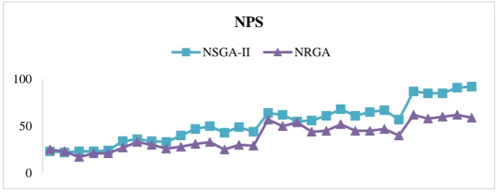
Figure 4, shows the comparison between NSGA-II and NRGA performance in number of Pareto solution index. As it can be seen in this figure, NSGA-II has a better performance than NRGA.
Figure 4. Performance comparison of the NSGA-II and NRGA based on NPS criteria
Figure 5, shows the comparison between NSGA-II and NRGA performance in CPU time index. As it can be seen in this figure, both algorithms have nearly identical performance on computational time.
0 200000 400000 600000
Diversity
NSGA-II NRGA
0 50 100
NPS
Figure 5. Efficiency comparison of the proposed algorithms based on computational time
5.4. Sensitivity Analysis
In addition, four one-way ANOVAs are used to statistically compare the performances of the two algorithms in terms of the four metric criteria. Tables 5-8 show the one-way ANOVA of the performance indices NPS, spacing, diversity, and CPU time at 95% confidence level along with the values of the corresponding p-values. Tables 5-8 show while there are significant differences between the two algorithms in terms of the means of NPS, spacing and diversity, and there are no significant differences among the two algorithms in term of the CPU time.
Table 5. The results of ANOVA for diversity criteria
Source DF SS MS F P-value
Factor 1 1868 1868 15.34 0
Error 58 7062 122
Total 59 8929
Table 6. The results of ANOVA for NPS criteria
Source DF SS MS F P-value
Factor 1 7871.2 7871.2 113.93 0
Error 58 4007.1 69.1
Total 59 11878.3
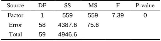
Table 7. The results of ANOVA for spacing criteria
Source DF SS MS F P-value
Factor 1 559 559 7.39 0
Error 58 4387.6 75.6
Total 59 4946.6
0 2000 4000 6000 8000 10000 12000
Time
Table 8. The results of ANOVA for computational time
Source 1DF 2SS 3MS 4F P-value
Factor 1 2254.7 2254.7 35.44 0.0049
Error 58 3689.9 63.6
Total 59 5944.6
1Degree of Freedom
2 Mean of Square error
3Sum of Square error
4F Distribution
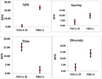
Also, for comparing the performances of the two algorithms in terms of the four metric criteria, Tukey test is used. Figure 6 shows the Tukey test of the performance indices NPS, spacing, diversity, and CPU time. The results show NSGA-II has better performance than NRGA in terms of the means of NPS, spacing and diversity with confidence level 95% and in CPU time, the result is reversed.
Figure 6. The results of Tukey tests for four metric criteria
6. Conclusions
The importance of network costs and responsiveness in supply chain management and reverse logistics activities has been significantly increased over the past years. Because of the increasing importance of customer service level as customer responsiveness and product quality as quality level in supply chain management and forward / reverse logistics activities, this paper presents a new mixed integer programming model for integrated forward / reverse logistics network including three objective functions. The first objective attempts to minimize the total cost of the supply chain network. The second objective attempts to maximize the customer service level in both forward and reverse networks. The third objective tries to minimize the total number of defects of in raw material obtained from suppliers and thus increase the quality level. The model application shows that the situation proposed results in a decrease of the total
0.00 10.00 20.00 30.00
NSGA-II NRGA
RP
D
NPS
0.00 5.00 10.00 15.00
NSGA-II NRGA
RPD
Spacing
0.00 5.00 10.00 15.00 20.00
NSGA-II NRGA
RP
D
Time
0.00 5.00 10.00 15.00 20.00
NSGA-II NRGA
RP
D
costs. To solve the proposed model, two meta-heuristic algorithms (NSGA-II and NRGA) are used. Besides, to evaluate the performance of the two algorithms some test problems are produced and analyzed with some metrics to determine which algorithm works better. Four quantitative performance metrics were used to analyze the diversity and convergence of algorithms. Finally, the outputs revealed that NSGA-II satisfy the criterion better than NRGA. The following approaches can be proposed to the future researchers:
Considering random or fuzzy parameter for the problem.
Considering other multi-objective meta-heuristic algorithms such as MOPSO or MOSA for solving the problem.
Developing of heuristic approach instead of generating random data in the initial segment.
Addressing the demand uncertainty and the supply of returned products in a multi-product integrated logistics network.
References
Al Jadaan, o., Rao, Rajamani, C. R., L. 2008. Non-dominated ranked genetic algorithm for solving multi-objective optimization problems: NRGA. Journal of Theoretical and Applied Information Technology, 2, 60-67.
Altiparmak, F., Gen, M., Lin, L., Paksoy, T. 2006. A genetic algorithm approach for multi-objective optimization of supply chain networks, Comput. Indus. Eng. 51, 197–216.
Amiri, A. 2006. Designing a distribution network in a supply chain system: formulation and efficient solution procedure, Eur. J. Oper. Res. 171 (2), 567–576.
Anne, M., Nicholas, L., Gicuru, I and Bula, O. (2016). Reverse logistics practices and their effect on competitiveness of food manufacturing firms in Kenya, International Journal of Economics, Finance and Management Sciences. Vol. 3: 678-684.
Binti, NNI, Moeinaddini, M., Ghazali, JB and Roslan, NFB. (2016). Reverse logistics in food industries: a case study in Malaysia, International Journal of Supply Chain Management. Vol. 5: 91-95.
Chan, F.T.S., Chung, S.H. 2004. A multi-criterion genetic algorithm for order distribution in a demand driven supply chain, Int. J. Comput. Integrat. Manufact. 17 (4), 339–351.
Davis, PS., Ray, TL. 1969. A branch-and-bound algorithm for the capacitated facilities location problem. Naval Research Logistics; 16: 331–44.
Deb, K., Pratap, A., Agarwal, S. and Meyarivan, T. 2002. A fast and elitist multi objective genetic algorithm: Nsga-ii, Evolutionary Computation, IEEE Transactions on, Vol. 6, No. 2, 182-197.
Demirel O.N., Gökçen, H. 2008. A mixed-integer programming model for remanufacturing in reverse logistics environment, Int. J. Adv. Manuf. Technol. 39 (11–12), 1197–1206.
Du, F., Evans, G.W. 2008. A bi-objective reverse logistics network analysis for post-sale service, Compute. Oper. Res. 35, 2617–2634.
Eroll, I., Ferrell, W.G. 2004. A methodology to support decision making a cross the supply chain of an industrial distributor, Int. J. Product. Econ. 89 (2004) 119-129.
Fleischmann, M., Beullens, P., Bloemhof-ruwaard, G.M., Wassenhove, L. 2001. The impact of product recovery on logistics network design, Product. Oper. Manag. 10, 156–173.
Franca, R.B., Jones, E.C., Richards, C.N., Carlson, J.P. 2009. Multi-objective stochastic supply chain modeling to evaluate tradeoffs between profit and quality, Int. J. Product. Econ. http://dx.doi.org/10.1016/j.ijpe.2009.09.005.
Gen, M., Altiparmak, F., Lin, L. 2006. A genetic algorithm for two-stage transportation problem using priority-based encoding, OR Spect. 28, 337–354.
Gen, M., Syarif, A. 2005. Hybrid genetic algorithm for multi-time period production/distribution planning, Compute. Indus. Eng. 48 (4), 799–809.
Giri, B.C. and Sharma, S. (2015). Optimizing a closed-loop supply chain with manufacturing defects and quality dependent return rate. Journal of Manufacturing Systems, Vol. 35, pp.92– 111.
Guillen, G., Mele, F.D., Bagajewicz, M.G., Espuna, A., Puigjaner, L. 2005. Multi-objectives supply chain design under uncertainty, Chem. Eng. Sci. 60, 1535–1553.
Huijun, S., Ziyou, G., Jianjun, W. 2008. A bi-level programming model and solution algorithm for the location of logistics distribution centers, Appl. Math. Modell. 32 (2008) 610–616.
Jacobs, F., Chase, R.B. 2008. Operations and Supply Management – The core, New York McGraw-Hill/Irwin.
Ko, H.J., Evans, G.W. 2007. A genetic-based heuristic for the dynamic integrated forward/reverse logistics network for 3PLs, Compute. Oper. Res. 34,346–366.
Krikke, H., Bloemhof-Ruwaard, J., Van Wassenhove, L.N. 2003. Concurrent product and closed-loop supply chain design with an application to refrigerators, Int. J. Prod. Res. 41 (16), 3689–3719.
Lee, D., Dong, M. 2008. A heuristic approach to logistics network design for end-of-lease computer products recovery, Transp. Res. Part E 44, 455–474.
Lee, D.H., Dong, M. 2009. Dynamic network design for reverse logistics operations under uncertainty, Transp. Res. Part E 45, 61–71.
Listes, O., Dekker, R. 2005. A stochastic approach to a case study for product recovery network design, Eur. J. Oper. Res. 160, 268–287.
Maosheng, T., Xiaoyun, G., Ling, Y., Haizhou, L., Wuyi, M., Zhen, Z and Jihong, C. (2016). Multi-objective optimization of injection molding process parameters in two stages for multiple quality characteristics and energy efficiency using Taguchi method and NSGA-II, Int J Adv Manuf Technol. Vol. 89: 241-254.
Melachrinoudis, E., Messac, A., Min, H. 2005. Consolidating a warehouse network: a physical programming approach, Int. J. Product. Econ. 97, 1–17.
Miranda, P.A., Garrido, R.A. 2004. Incorporating inventory control decisions into a strategic distribution network design model with stochastic demand, Transp. Res. Part E 40,183–207.
Pishvaee, M.R., Farahani, R.Z., Dullaert, W. 2010. A memetic algorithm for bi-objective integrated forward/reverse logistics network design, Compute. Oper. Res37 (6), 1100–111.
Pishvaee, M.R., Kianfar, K., Karimi, B. 2010. Reverse logistics network design using simulated annealing, Int. J. Adv. Manuf. Technol. 47, 269–281.
Rajagopal, P., Sundram, VPK and Naidu, BM. (2015). Future directions of reverse logistics in gaining competitive advantages: a review of literature, International Journal Supply Chain Management, Vol. 4: 39-48.
Ramezani, M. and Bashiri, M. and Tavakkoli-Moghaddam, R. 2013. A new multi-objective stochastic model for a forward/reverse logistic network design with responsiveness and quality level. http://www.elsevier.com/locate/apm, 37(4), PP.535–344.
Sabri, E.H., Beamon, B.M. 2000. A multi-objective approach to simultaneous strategic and operational planning in supply chain design, OMEGA 28, 581–598.
Salema, M.I., Po’voa, A.P.B., Novais, A.Q. 2006. A warehouse-based design model for reverse logistics, J. Oper. Res. Soc. 57 (6), 615–629.
Salema, M.I.G., Barbosa-Povoa, A.P., Novais, A.Q. 2007. An optimization model for the design of a capacitated multi-product reverse logistics network with uncertainty, Eur. J. Oper. Res. 179, 1063–1077.
Selim, H., Ozkarahan, I. 2008. A supply chain distribution network design model: an interactive fuzzy goal programming-based solution approach, Int. J. Adv. Manuf. Technol. 36, 401–418.
Syarif, Y.S., Yun, A., Gen, M. 2002. Study on multi-stage logistics chain network: a spanning tree-based genetic algorithm approach, Compute. Indus. Eng. 43, 299–314.
Tavakkoli-Moghaddam, R., Azarkish, M. and Sadeghnejad- Barkousaraie, A. 2011. Solving a multi-objective job shop scheduling problem with sequence-dependent setup times by a pareto archive pso combined with genetic operators and vns, The International Journal of Advanced Manufacturing Technology, Vol. 53, No. 5-8, 733-750.
Tsiakis, P., Papageorgiou, L.G. 2008. Optimal production allocation and distribution supply chain networks, Int. J. Product. Econ. 111, 468–483.
Uster, H., Easwaran, G., Akçali, E., Çetinkaya, S. 2007. Benders decomposition with alternative multiple cuts for a multi-product closed-loop supply chain network design model, Naval Res. Logist. 54, 890–907.
Wang, H.F., Hsu, H.W. 2010. A closed-loop logistic model with a spanning-tree based genetic algorithm, Compute. Oper. Res. 37, 376–389.