www.earth-syst-sci-data.net/8/605/2016/ doi:10.5194/essd-8-605-2016
© Author(s) 2016. CC Attribution 3.0 License.
Global Carbon Budget 2016
Corinne Le Quéré1, Robbie M. Andrew2, Josep G. Canadell3, Stephen Sitch4, Jan Ivar Korsbakken2,
Glen P. Peters2, Andrew C. Manning5, Thomas A. Boden6, Pieter P. Tans7, Richard A. Houghton8,
Ralph F. Keeling9, Simone Alin10, Oliver D. Andrews1, Peter Anthoni11, Leticia Barbero12,13,
Laurent Bopp14, Frédéric Chevallier14, Louise P. Chini15, Philippe Ciais14, Kim Currie16,
Christine Delire17, Scott C. Doney18, Pierre Friedlingstein19, Thanos Gkritzalis20, Ian Harris21,
Judith Hauck22, Vanessa Haverd23, Mario Hoppema22, Kees Klein Goldewijk24, Atul K. Jain25,
Etsushi Kato26, Arne Körtzinger27, Peter Landschützer28, Nathalie Lefèvre29, Andrew Lenton30,
Sebastian Lienert31,32, Danica Lombardozzi33, Joe R. Melton34, Nicolas Metzl29, Frank Millero35,
Pedro M. S. Monteiro36, David R. Munro37, Julia E. M. S. Nabel28, Shin-ichiro Nakaoka38,
Kevin O’Brien39, Are Olsen40, Abdirahman M. Omar40, Tsuneo Ono41, Denis Pierrot12,13,
Benjamin Poulter42,43, Christian Rödenbeck44, Joe Salisbury45, Ute Schuster4, Jörg Schwinger46,
Roland Séférian17, Ingunn Skjelvan46, Benjamin D. Stocker47, Adrienne J. Sutton39,10, Taro Takahashi48,
Hanqin Tian49, Bronte Tilbrook50, Ingrid T. van der Laan-Luijkx51, Guido R. van der Werf52,
Nicolas Viovy14, Anthony P. Walker53, Andrew J. Wiltshire54, and Sönke Zaehle44
1Tyndall Centre for Climate Change Research, University of East Anglia, Norwich Research Park,
Norwich, NR4 7TJ, UK
2Center for International Climate and Environmental Research – Oslo (CICERO), Oslo, Norway 3Global Carbon Project, CSIRO Oceans and Atmosphere, GPO Box 3023, Canberra, ACT 2601, Australia
4College of Life and Environmental Sciences, University of Exeter, Exeter, EX4 4RJ, UK
5Centre for Ocean and Atmospheric Sciences, School of Environmental Sciences, University of East Anglia,
Norwich Research Park, Norwich, NR4 7TJ, UK
6Carbon Dioxide Information Analysis Center (CDIAC), Oak Ridge National Laboratory, Oak Ridge, TN, USA 7National Oceanic & Atmospheric Administration, Earth System Research Laboratory (NOAA/ESRL),
Boulder, CO 80305, USA
8Woods Hole Research Center (WHRC), Falmouth, MA 02540, USA
9University of California, San Diego, Scripps Institution of Oceanography, La Jolla, CA 92093-0244, USA 10National Oceanic & Atmospheric Administration/Pacific Marine Environmental Laboratory (NOAA/PMEL),
7600 Sand Point Way NE, Seattle, WA 98115, USA
11Karlsruhe Institute of Technology, Institute of Meteorology and Climate Research/Atmospheric
Environmental Research, 82467 Garmisch-Partenkirchen, Germany
12Cooperative Institute for Marine and Atmospheric Studies, Rosenstiel School for Marine and
Atmospheric Science, University of Miami, Miami, FL 33149, USA
13National Oceanic & Atmospheric Administration/Atlantic Oceanographic & Meteorological Laboratory
(NOAA/AOML), Miami, FL 33149, USA
14Laboratoire des Sciences du Climat et de l’Environnement, Institut Pierre-Simon Laplace,
CEA-CNRS-UVSQ, CE Orme des Merisiers, 91191 Gif sur Yvette CEDEX, France
15Department of Geographical Sciences, University of Maryland, College Park, MD 20742, USA 16National Institute of Water and Atmospheric Research (NIWA), Dunedin 9054, New Zealand 17Centre National de Recherche Météorologique, Unite mixte de recherche 3589 Météo-France/CNRS,
42 Avenue Gaspard Coriolis, 31100 Toulouse, France
18Woods Hole Oceanographic Institution (WHOI), Woods Hole, MA 02543, USA
19College of Engineering, Mathematics and Physical Sciences, University of Exeter, Exeter, EX4 4QF, UK 20Flanders Marine Institute, InnovOcean, Wandelaarkaai 7, 8400 Ostend, Belgium
22Alfred Wegener Institute Helmholtz Centre for Polar and Marine Research, Postfach 120161,
27515 Bremerhaven, Germany
23CSIRO Oceans and Atmosphere, GPO Box 1700, Canberra, ACT 2601, Australia 24PBL Netherlands Environmental Assessment Agency, The Hague/Bilthoven and Utrecht University,
Utrecht, the Netherlands
25Department of Atmospheric Sciences, University of Illinois, Urbana, IL 61821, USA 26Institute of Applied Energy (IAE), Minato-ku, Tokyo 105-0003, Japan
27GEOMAR Helmholtz Centre for Ocean Research Kiel, Düsternbrooker Weg 20, 24105 Kiel, Germany 28Max Planck Institute for Meteorology, Bundesstr. 53, 20146 Hamburg, Germany
29Sorbonne Universités (UPMC, Univ Paris 06), CNRS, IRD, MNHN, LOCEAN/IPSL Laboratory,
75252 Paris, France
30CSIRO Oceans and Atmosphere, P.O. Box 1538, Hobart, TAS, Australia
31Climate and Environmental Physics, Physics Institute, University of Bern, Bern, Switzerland 32Oeschger Centre for Climate Change Research, University of Bern, Bern, Switzerland
33National Center for Atmospheric Research, Climate and Global Dynamics, Terrestrial Sciences Section,
Boulder, CO 80305, USA
34Climate Research Division, Environment and Climate Change Canada, Victoria, Canada
35Department of Ocean Sciences, RSMAS/MAC, University of Miami, 4600 Rickenbacker Causeway, Miami,
FL 33149, USA
36Ocean Systems and Climate, CSIR-CHPC, Cape Town, 7700, South Africa 37Department of Atmospheric and Oceanic Sciences and Institute of Arctic and Alpine Research,
University of Colorado, Campus Box 450, Boulder, CO 80309-0450, USA
38Center for Global Environmental Research, National Institute for Environmental Studies (NIES),
16-2 Onogawa, Tsukuba, Ibaraki 305-8506, Japan
39Joint Institute for the Study of the Atmosphere and Ocean, University of Washington, Seattle,
WA 98195, USA
40Geophysical Institute, University of Bergen and Bjerknes Centre for Climate Research, Allégaten 70,
5007 Bergen, Norway
41National Research Institute for Far Sea Fisheries, Japan Fisheries Research and Education Agency 2-12-4
Fukuura, Kanazawa-Ku, Yokohama 236-8648, Japan
42NASA Goddard Space Flight Center, Biospheric Science Laboratory, Greenbelt, MD 20771, USA 43Department of Ecology, Montana State University, Bozeman, MT 59717, USA
44Max Planck Institute for Biogeochemistry, P.O. Box 600164, Hans-Knöll-Str. 10, 07745 Jena, Germany 45University of New Hampshire, Ocean Process Analysis Laboratory, 161 Morse Hall, 8 College Road,
Durham, NH 03824, USA
46Uni Research Climate, Bjerknes Centre for Climate Research, Nygårdsgaten 112, 5008 Bergen, Norway 47Imperial College London, Life Science Department, Silwood Park, Ascot, Berkshire, SL5 7PY, UK
48Lamont-Doherty Earth Observatory of Columbia University, Palisades, NY 10964, USA
49School of Forestry and Wildlife Sciences, Auburn University, 602 Ducan Drive, Auburn, AL 36849, USA 50CSIRO Oceans and Atmosphere and Antarctic Climate and Ecosystems Cooperative Research Centre,
Hobart, TAS, Australia
51Department of Meteorology and Air Quality, Wageningen University & Research, P.O. Box 47,
6700AA Wageningen, the Netherlands
52Faculty of Earth and Life Sciences, VU University Amsterdam, Amsterdam, the Netherlands 53Environmental Sciences Division & Climate Change Science Institute, Oak Ridge National Laboratory,
Oak Ridge, TN, USA
54Met Office Hadley Centre, FitzRoy Road, Exeter, EX1 3PB, UK
Correspondence to:Corinne Le Quéré ([email protected])
Received: 5 October 2016 – Published in Earth Syst. Sci. Data Discuss.: 12 October 2016 Revised: 12 October 2016 – Accepted: 18 October 2016 – Published: 14 November 2016
Abstract. Accurate assessment of anthropogenic carbon dioxide (CO2) emissions and their redistribution
change. Here we describe data sets and methodology to quantify all major components of the global carbon bud-get, including their uncertainties, based on the combination of a range of data, algorithms, statistics, and model estimates and their interpretation by a broad scientific community. We discuss changes compared to previous estimates and consistency within and among components, alongside methodology and data limitations. CO2
emissions from fossil fuels and industry (EFF) are based on energy statistics and cement production data,
respec-tively, while emissions from land-use change (ELUC), mainly deforestation, are based on combined evidence
from land-cover change data, fire activity associated with deforestation, and models. The global atmospheric CO2concentration is measured directly and its rate of growth (GATM) is computed from the annual changes
in concentration. The mean ocean CO2sink (SOCEAN) is based on observations from the 1990s, while the
an-nual anomalies and trends are estimated with ocean models. The variability inSOCEAN is evaluated with data
products based on surveys of ocean CO2 measurements. The global residual terrestrial CO2 sink (SLAND) is
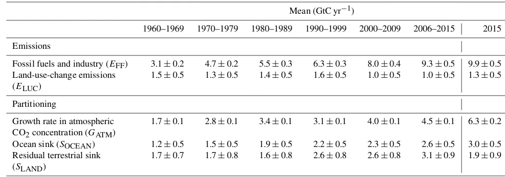
estimated by the difference of the other terms of the global carbon budget and compared to results of indepen-dent dynamic global vegetation models. We compare the mean land and ocean fluxes and their variability to estimates from three atmospheric inverse methods for three broad latitude bands. All uncertainties are reported as±1σ, reflecting the current capacity to characterise the annual estimates of each component of the global car-bon budget. For the last decade available (2006–2015),EFFwas 9.3±0.5 GtC yr−1,ELUC1.0±0.5 GtC yr−1,
GATM4.5±0.1 GtC yr−1,SOCEAN2.6±0.5 GtC yr−1, andSLAND3.1±0.9 GtC yr−1. For year 2015 alone, the
growth inEFFwas approximately zero and emissions remained at 9.9±0.5 GtC yr−1, showing a slowdown in
growth of these emissions compared to the average growth of 1.8 % yr−1 that took place during 2006–2015. Also, for 2015,ELUCwas 1.3±0.5 GtC yr−1,GATMwas 6.3±0.2 GtC yr−1,SOCEAN was 3.0±0.5 GtC yr−1,
andSLANDwas 1.9±0.9 GtC yr−1.GATMwas higher in 2015 compared to the past decade (2006–2015),
reflect-ing a smallerSLANDfor that year. The global atmospheric CO2concentration reached 399.4±0.1 ppm averaged
over 2015. For 2016, preliminary data indicate the continuation of low growth inEFFwith+0.2 % (range of −1.0 to+1.8 %) based on national emissions projections for China and USA, and projections of gross domestic product corrected for recent changes in the carbon intensity of the economy for the rest of the world. In spite of the low growth ofEFFin 2016, the growth rate in atmospheric CO2concentration is expected to be relatively
high because of the persistence of the smaller residual terrestrial sink (SLAND) in response to El Niño conditions of 2015–2016. From this projection ofEFFand assumed constantELUCfor 2016, cumulative emissions of CO2
will reach 565±55 GtC (2075±205 GtCO2) for 1870–2016, about 75 % fromEFFand 25 % fromELUC. This
living data update documents changes in the methods and data sets used in this new carbon budget compared with previous publications of this data set (Le Quéré et al., 2015b, a, 2014, 2013). All observations presented here can be downloaded from the Carbon Dioxide Information Analysis Center (doi:10.3334/CDIAC/GCP_2016).
1 Introduction
The concentration of carbon dioxide (CO2) in the atmosphere
has increased from approximately 277 parts per million (ppm) in 1750 (Joos and Spahni, 2008), the beginning of the industrial era, to 399.4±0.1 ppm in 2015 (Dlugokencky and Tans, 2016). The Mauna Loa station, which holds the longest running record of direct measurements of atmospheric CO2
concentration (Tans and Keeling, 2014), went above 400 ppm for the first time in May 2013 (Scripps, 2013). The global monthly average concentration was above 400 ppm in March through May 2015 and again since November 2015 (Dlu-gokencky and Tans, 2016; Fig. 1). The atmospheric CO2
increase above pre-industrial levels was, initially, primar-ily caused by the release of carbon to the atmosphere from deforestation and other land-use-change activities (Ciais et al., 2013). While emissions from fossil fuels started before the industrial era, they only became the dominant source of anthropogenic emissions to the atmosphere from around
1920, and their relative share has continued to increase until present. Anthropogenic emissions occur on top of an active natural carbon cycle that circulates carbon between the reser-voirs of the atmosphere, ocean, and terrestrial biosphere on timescales from sub-daily to millennia, while exchanges with geologic reservoirs occur at longer timescales (Archer et al., 2009).
The global carbon budget presented here refers to the mean, variations, and trends in the perturbation of CO2 in
the atmosphere, referenced to the beginning of the industrial era. It quantifies the input of CO2to the atmosphere by
emis-sions from human activities, the growth rate of atmospheric CO2concentration, and the resulting changes in the storage
of carbon in the land and ocean reservoirs in response to in-creasing atmospheric CO2 levels, climate change and
1960 1970 1980 1990 2000 2010 2020 310
320 330 340 350 360 370 380 390 400 410
Time (yr)
Atmospheric CO
2
concentration (ppm)
Seasonally corrected trend:
Monthly mean:
Scripps Institution of Oceanography (Keeling et al., 1976) NOAA/ESRL (Dlugokencky & Tans, 2016)
NOAA/ESRL
Figure 1. Surface average atmospheric CO2 concentration,
de-seasonalised (ppm). The 1980–2016 monthly data are from NOAA/ESRL (Dlugokencky and Tans, 2016) and are based on an average of direct atmospheric CO2 measurements from
mul-tiple stations in the marine boundary layer (Masarie and Tans, 1995). The 1958–1979 monthly data are from the Scripps Institu-tion of Oceanography, based on an average of direct atmospheric CO2measurements from the Mauna Loa and South Pole stations (Keeling et al., 1976). To take into account the difference of mean CO2between the NOAA/ESRL and the Scripps station networks
used here, the Scripps surface average (from two stations) was har-monised to match the NOAA/ESRL surface average (from multiple stations) by adding the mean difference of 0.542 ppm, calculated here from overlapping data during 1980–2012. The mean seasonal cycle is also shown from 1980 (in pink).
to changes in climate, CO2, and land-use-change drivers, and
the permissible emissions for a given climate stabilisation target.
The components of the CO2budget that are reported
an-nually in this paper include separate estimates for the CO2
emissions from (1) fossil fuel combustion and oxidation and cement production (EFF; GtC yr−1) and (2) the emissions
re-sulting from deliberate human activities on land leading to land-use change (ELUC; GtC yr−1), as well as their
parti-tioning among (3) the growth rate of atmospheric CO2
con-centration (GATM; GtC yr−1), and the uptake of CO2by the
“CO2sinks” in (4) the ocean (SOCEAN; GtC yr−1) and (5) on
land (SLAND; GtC yr−1). The CO2 sinks as defined here
in-clude the response of the land and ocean to elevated CO2
and changes in climate and other environmental conditions. The global emissions and their partitioning among the atmo-sphere, ocean, and land are in balance:
EFF+ELUC=GATM+SOCEAN+SLAND. (1)
GATM is usually reported in ppm yr−1, which we
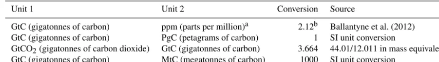
con-vert to units of carbon mass per year, GtC yr−1, using 1 ppm=2.12 GtC (Ballantyne et al., 2012; Prather et al., 2012; Table 1). We also include a quantification of EFFby
Fossil fuels & industry
9.3 ± 0.5 Land-use change
1.0 ± 0.5
Land sink
3.1 ± 0.9
Ocean sink
2.6 ± 0.5
Atmospheric growth
4.5 ± 0.1
Geological reservoirs
Global carbon dioxide budget
(gigatonnes of carbon per year)
2006-2015
© Global C arbon P
roject 2014 Desig
ned by the IGBP
Figure 2.Schematic representation of the overall perturbation of the global carbon cycle caused by anthropogenic activities, av-eraged globally for the decade 2006–2015. The arrows represent emission from fossil fuels and industry (EFF), emissions from
de-forestation and other land-use change (ELUC), the growth rate in
atmospheric CO2concentration (GATM), and the uptake of carbon
by the “sinks” in the ocean (SOCEAN) and land (SLAND) reservoirs.
All fluxes are in units of GtC yr−1, with uncertainties reported as
±1σ (68 % confidence that the real value lies within the given in-terval) as described in the text. This figure is an update of one pre-pared by the International Geosphere-Biosphere Programme for the Global Carbon Project (GCP), first presented in Le Quéré (2009).
country, computed with both territorial and consumption-based accounting (see Sect. 2).
Equation (1) partly omits two kinds of processes. The first is the net input of CO2to the atmosphere from the chemical
oxidation of reactive carbon-containing gases from sources other than the combustion of fossil fuels (e.g. fugitive anthro-pogenic CH4 emissions, industrial processes, and biogenic
emissions from changes in vegetation, fires, wetlands), pri-marily methane (CH4), carbon monoxide (CO), and volatile
organic compounds such as isoprene and terpene (Gonzalez-Gaya et al., 2016). CO emissions are currently implicit in
EFF, while fugitive anthropogenic CH4 emissions are not
and thus their inclusion would result in a small increase in
EFF. The second is the anthropogenic perturbation to carbon cycling in terrestrial freshwaters, estuaries, and coastal ar-eas, which modifies lateral fluxes from land ecosystems to the open ocean; the evasion of CO2 flux from rivers, lakes,
and estuaries to the atmosphere; and the net air–sea anthro-pogenic CO2flux of coastal areas (Regnier et al., 2013). The
inclusion of freshwater fluxes of anthropogenic CO2would
Table 1.Factors used to convert carbon in various units (by convention, unit 1=unit 2·conversion).
Unit 1 Unit 2 Conversion Source
GtC (gigatonnes of carbon) ppm (parts per million)a 2.12b Ballantyne et al. (2012)
GtC (gigatonnes of carbon) PgC (petagrams of carbon) 1 SI unit conversion
GtCO2(gigatonnes of carbon dioxide) GtC (gigatonnes of carbon) 3.664 44.01/12.011 in mass equivalent
GtC (gigatonnes of carbon) MtC (megatonnes of carbon) 1000 SI unit conversion
aMeasurements of atmospheric CO
2concentration have units of dry-air mole fraction. “ppm” is an abbreviation for micromole per mole of dry air.bThe use of a factor of 2.12 assumes that all the atmosphere is well mixed within one year. In reality, only the troposphere is well mixed and the growth rate of CO2 concentration in the less well-mixed stratosphere is not measured by sites from the NOAA network. Using a factor of 2.12 makes the approximation that the growth rate of CO2concentration in the stratosphere equals that of the troposphere on a yearly basis.
affect the other terms. These flows are omitted in the absence of annual information on the natural vs. anthropogenic per-turbation terms of these loops of the carbon cycle, and they are discussed in Sect. 2.7.
The CO2 budget has been assessed by the
Intergovern-mental Panel on Climate Change (IPCC) in all assessment reports (Ciais et al., 2013; Denman et al., 2007; Prentice et al., 2001; Schimel et al., 1995; Watson et al., 1990), as well as by others (e.g. Ballantyne et al., 2012). These assessments included budget estimates for the decades of the 1980s and 1990s (Denman et al., 2007) and, most recently, the period 2002–2011 (Ciais et al., 2013). The IPCC methodology has been adapted and used by the Global Carbon Project (GCP, http://www.globalcarbonproject.org), which has coordinated a cooperative community effort for the annual publication of global carbon budgets up to year 2005 (Raupach et al., 2007; including fossil emissions only), year 2006 (Canadell et al., 2007), year 2007 (published online; GCP, 2007), year 2008 (Le Quéré et al., 2009), year 2009 (Friedlingstein et al., 2010), year 2010 (Peters et al., 2012b), year 2012 (Le Quéré et al., 2013; Peters et al., 2013), year 2013 (Le Quéré et al., 2014), year 2014 (Friedlingstein et al., 2014; Le Quéré et al., 2015b), and most recently year 2015 (Jackson et al., 2016; Le Quéré et al., 2015a). Each of these papers updated pre-vious estimates with the latest available information for the entire time series. From 2008, these publications projected fossil fuel emissions for one additional year.
We adopt a range of±1 standard deviation (σ) to report the uncertainties in our estimates, representing a likelihood of 68 % that the true value will be within the provided range if the errors have a Gaussian distribution. This choice reflects the difficulty of characterising the uncertainty in the CO2
fluxes between the atmosphere and the ocean and land reser-voirs individually, particularly on an annual basis, as well as the difficulty of updating the CO2emissions from land-use
change. A likelihood of 68 % provides an indication of our current capability to quantify each term and its uncertainty given the available information. For comparison, the Fifth Assessment Report of the IPCC (AR5) generally reported a likelihood of 90 % for large data sets whose uncertainty is well characterised, or for long time intervals less affected by year-to-year variability. Our 68 % uncertainty value is near
the 66 % which the IPCC characterises as “likely” for values falling into the±1σinterval. The uncertainties reported here combine statistical analysis of the underlying data and ex-pert judgement of the likelihood of results lying outside this range. The limitations of current information are discussed in the paper and have been examined in detail elsewhere (Bal-lantyne et al., 2015).
All quantities are presented in units of gigatonnes of car-bon (GtC, 1015gC), which is the same as petagrams of car-bon (PgC; Table 1). Units of gigatonnes of CO2 (or billion
tonnes of CO2) used in policy are equal to 3.664 multiplied
by the value in units of GtC.
This paper provides a detailed description of the data sets and methodology used to compute the global carbon bud-get estimates for the period pre-industrial (1750) to 2015 and in more detail for the period 1959 to 2015. We also provide decadal averages starting in 1960 including the last decade (2006–2015), results for the year 2015, and a projection for year 2016. Finally, we provide cumulative emissions from fossil fuels and land-use change since year 1750, the pre-industrial period, and since year 1870, the reference year for the cumulative carbon estimate used by the IPCC (AR5) based on the availability of global tem-perature data (Stocker et al., 2013). This paper will be updated every year using the format of “living data” to keep a record of budget versions and the changes in new data, revision of data, and changes in methodology that lead to changes in estimates of the carbon budget. Addi-tional materials associated with the release of each new ver-sion will be posted at the Global Carbon Project (GCP) website (http://www.globalcarbonproject.org/carbonbudget), with fossil fuel emissions also available through the Global Carbon Atlas (http://www.globalcarbonatlas.org). With this approach, we aim to provide the highest transparency and traceability in the reporting of CO2, the key driver of climate
change.
2 Methods
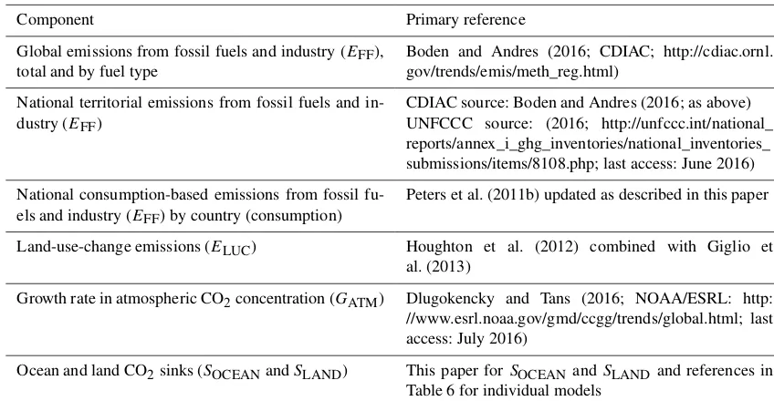
Table 2.How to cite the individual components of the global carbon budget presented here.
Component Primary reference
Global emissions from fossil fuels and industry (EFF),
total and by fuel type
Boden and Andres (2016; CDIAC; http://cdiac.ornl. gov/trends/emis/meth_reg.html)
National territorial emissions from fossil fuels and in-dustry (EFF)
CDIAC source: Boden and Andres (2016; as above) UNFCCC source: (2016; http://unfccc.int/national_ reports/annex_i_ghg_inventories/national_inventories_ submissions/items/8108.php; last access: June 2016)
National consumption-based emissions from fossil fu-els and industry (EFF) by country (consumption)
Peters et al. (2011b) updated as described in this paper
Land-use-change emissions (ELUC) Houghton et al. (2012) combined with Giglio et
al. (2013)
Growth rate in atmospheric CO2concentration (GATM) Dlugokencky and Tans (2016; NOAA/ESRL: http:
//www.esrl.noaa.gov/gmd/ccgg/trends/global.html; last access: July 2016)
Ocean and land CO2sinks (SOCEANandSLAND) This paper forSOCEAN andSLANDand references in
Table 6 for individual models
thus mainly one of synthesis, where results from individual groups are collated, analysed, and evaluated for consistency. We facilitate access to original data with the understanding that primary data sets will be referenced in future work (see Table 2 for how to cite the data sets). Descriptions of the measurements, models, and methodologies follow below and in-depth descriptions of each component are described else-where.
This is the 11th version of the global carbon budget and the fifth revised version in the format of a living data up-date. It builds on the latest published global carbon budget of Le Quéré et al. (2015a). The main changes are (1) the in-clusion of data to year 2015 (inclusive) and a projection for fossil fuel emissions for year 2016; (2) the introduction of a projection for the full carbon budget for year 2016 using our fossil fuel projection, combined with preliminary data (Dlu-gokencky and Tans, 2016) and analysis by others (Betts et al., 2016) of the growth rate in atmospheric CO2
concentra-tion; and (3) the use of BP data from 1990 (BP, 2016b) to estimate emissions in China to ensure all recent revisions in Chinese statistics are incorporated. The main methodological differences between annual carbon budgets are summarised in Table 3.
2.1 CO2emissions from fossil fuels and industry (EFF)
2.1.1 Emissions from fossil fuels and industry and their uncertainty
The calculation of global and national CO2emissions from
fossil fuels, including gas flaring and cement production (EFF), relies primarily on energy consumption data,
specif-ically data on hydrocarbon fuels, collated and archived by
several organisations (Andres et al., 2012). These include the Carbon Dioxide Information Analysis Center (CDIAC), the International Energy Agency (IEA), the United Nations (UN), the United States Department of Energy (DoE) En-ergy Information Administration (EIA), and more recently also the Planbureau voor de Leefomgeving (PBL) Nether-lands Environmental Assessment Agency. Where available, we use national emissions estimated by the countries them-selves and reported to the UNFCCC for the period 1990– 2014 (40 countries). We assume that national emissions re-ported to the UNFCCC are the most accurate because na-tional experts have access to addina-tional and country-specific information, and because these emission estimates are peri-odically audited for each country through an established in-ternational methodology overseen by the UNFCCC. We also use global and national emissions estimated by CDIAC (Bo-den and Andres, 2016). The CDIAC emission estimates are the only data set that extends back in time to 1751 with con-sistent and well-documented emissions from fossil fuels, ce-ment production, and gas flaring for all countries and their uncertainty (Andres et al., 2014, 2012, 1999); this makes the data set a unique resource for research of the carbon cycle during the fossil fuel era.
The global emissions presented here are based on CDIAC’s analysis, which provides an internally consistent global estimate including bunker fuels, minimising the ef-fects of lower-quality energy trade data. Thus, the compari-son of global emissions with previous annual carbon budgets is not influenced by the use of national data from UNFCCC reports.
Table 4.Data sources used to compute each component of the global carbon budget.
Component Process Data source Data reference
EFF (global and
CDIAC national)
Fossil fuel combustion and gas flaring
UN Statistics Division to 2013 UN (2015a, b)
BP for 2014–2015 BP (BP, 2016b)
Cement production US Geological Survey USGS (2016a, b)
ELUC Land-cover change
(deforesta-tion, afforesta(deforesta-tion, and forest regrowth)
Forest Resource Assessment (FRA) of the Food and Agricul-ture Organization (FAO)
FAO (2010)
Wood harvest FAO Statistics Division FAOSTAT (2010)
Shifting agriculture FAO FRA and Statistics
Divi-sion
FAO (2010) FAOSTAT (2010)
Interannual variability from peat fires and climate–land management interactions (1997–2013)
Global Fire Emissions Database (GFED4)
Giglio et al. (2013)
GATM Change in atmospheric CO2
concentration
1959–1980: CO2 Program at Scripps Institution of Oceanog-raphy and other research groups
Keeling et al. (1976)
1980–2015: US National
Oceanic and Atmospheric
Administration Earth System Research Laboratory
Dlugokencky and Tans (2016) Ballantyne et al. (2012)
SOCEAN Uptake of anthropogenic CO2 1990–1999 average: indirect
es-timates based on CFCs, atmo-spheric O2, and other tracer ob-servations
Manning and Keeling (2006) McNeil et al. (2003)
Mikaloff Fletcher et al. (2006) as assessed by the IPCC in Den-man et al. (2007)
Impact of increasing atmo-spheric CO2, climate, and
vari-ability
Ocean models Table 6
SLAND Response of land vegetation to
increasing atmospheric CO2
concentration,
climate and variability, and other environmental changes
Budget residual
ble 4). When necessary, fuel masses/volumes are converted to fuel energy content using coefficients provided by the UN and then to CO2emissions using conversion factors that take
into account the relationship between carbon content and en-ergy (heat) content of the different fuel types (coal, oil, gas, gas flaring) and the combustion efficiency (to account, for example, for soot left in the combustor or fuel otherwise lost or discharged without oxidation). Most data on energy consumption and fuel quality (carbon content and heat con-tent) are available at the country level (UN, 2015a). In gen-eral, CO2emissions for equivalent primary energy
consump-tion are about 30 % higher for coal compared to oil, and 70 % higher for coal compared to natural gas (Marland et al., 2007).
differ-ence). We propagate these new estimates for China through to the global total to ensure consistency.
Our emission totals for the UNFCCC-reporting countries were recorded as in the UNFCCC submissions, which have a slightly larger system boundary than CDIAC. Additional emissions come from carbonates other than in cement manu-facture, and thus UNFCCC totals will be slightly higher than CDIAC totals in general, although there are multiple sources of differences. We use the CDIAC method to report emis-sions by fuel type (e.g. all coal oxidation is reported under “coal”, regardless of whether oxidation results from combus-tion as an energy source), which differs slightly from UN-FCCC.
For the most recent 1–2 years when the UNFCCC esti-mates (1 year) and UN statistics (2 years) used by CDIAC are not yet available, we generated preliminary estimates based on the BP annual energy review by applying the growth rates of energy consumption (coal, oil, gas) for 2015 to the na-tional and global emissions from the UN nana-tional data in 2014, and for 2014 and 2015 to the CDIAC national and global emissions in 2013. BP’s sources for energy statis-tics overlap with those of the UN data but are compiled more rapidly from about 70 countries covering about 96 % of global emissions. We use the BP values only for the year-to-year rate of change, because the rates of change are less uncertain than the absolute values and to avoid discontinu-ities in the time series when linking the UN-based data with the BP data. These preliminary estimates are replaced by the more complete UNFCCC or CDIAC data based on UN statis-tics when they become available. Past experience and work by others (Andres et al., 2014; Myhre et al., 2009) show that projections based on the BP rate of change are within the un-certainty provided (see Sect. 3.2 and Supplement from Peters et al., 2013).
Estimates of emissions from cement production by CDIAC are based on data on growth rates of cement produc-tion from the US Geological Survey up to year 2013 (USGS, 2016a). For 2014 and 2015 we use estimates of cement pro-duction made by the USGS for the top 18 countries (rep-resenting 85 % of global production; USGS, 2016b), while for all other countries we use the 2013 values (zero growth). Some fraction of the CaO and MgO in cement is returned to the carbonate form during cement weathering, but this is neglected here.
Estimates of emissions from gas flaring by CDIAC are cal-culated in a similar manner to those from solid, liquid, and gaseous fuels and rely on the UN energy statistics to supply the amount of flared or vented fuel. For the most recent 1–2 emission years, flaring is assumed constant from the most re-cent available year of data (2014 for countries that report to the UNFCCC, and 2013 for the remainder). The basic data on gas flaring report atmospheric losses during petroleum pro-duction and processing that have large uncertainty and do not distinguish between gas that is flared as CO2or vented as
CH4. Fugitive emissions of CH4from the so-called upstream
sector (e.g. coal mining and natural gas distribution) are not included in the accounts of CO2emissions except to the
ex-tent that they are captured in the UN energy data and counted as gas “flared or lost”.
The published CDIAC data set includes 255 countries and regions. This list includes countries that no longer exist, such as the USSR and East Pakistan. For the carbon budget, we reduce the list to 219 countries by reallocating emissions to the currently defined territories. This involved both aggrega-tion and disaggregaaggrega-tion, and does not change global emis-sions. Examples of aggregation include merging East and West Germany to the currently defined Germany. Examples of disaggregation include reallocating the emissions from the former USSR to the resulting independent countries. For dis-aggregation, we use the emission shares when the current territories first appeared. The disaggregated estimates should be treated with care when examining countries’ emissions trends prior to their disaggregation. For the most recent years, 2014 and 2015, the BP statistics are more aggregated, but we retain the detail of CDIAC by applying the growth rates of each aggregated region in the BP data set to its constituent individual countries in CDIAC.
Estimates of CO2emissions show that the global total of
emissions is not equal to the sum of emissions from all coun-tries. This is largely attributable to emissions that occur in international territory, in particular the combustion of fuels used in international shipping and aviation (bunker fuels), where the emissions are included in the global totals but are not attributed to individual countries. In practice, the emis-sions from international bunker fuels are calculated based on where the fuels were loaded, but they are not included with national emissions estimates. Other differences occur be-cause globally the sum of imports in all countries is not equal to the sum of exports and because of inconsistent national re-porting, differing treatment of oxidation of non-fuel uses of hydrocarbons (e.g. as solvents, lubricants, feedstocks), and changes in stock (Andres et al., 2012).
The uncertainty in the annual emissions from fossil fuels and industry for the globe has been estimated at±5 % (scaled down from the published±10 % at±2σ to the use of±1σ
iden-tified suggesting China’s emissions could be overestimated in published studies (Liu et al., 2015). Generally, emissions from mature economies with good statistical bases have an uncertainty of only a few percent (Marland, 2008). Further research is needed before we can quantify the time evolu-tion of the uncertainty, as well as its temporal error correla-tion structure. We note that even if they are presented as 1σ
estimates, uncertainties in emissions are likely to be mainly country-specific systematic errors related to underlying bi-ases of energy statistics and to the accounting method used by each country. We assign a medium confidence to the re-sults presented here because they are based on indirect esti-mates of emissions using energy data (Durant et al., 2011). There is only limited and indirect evidence for emissions, although there is a high agreement among the available es-timates within the given uncertainty (Andres et al., 2014, 2012), and emission estimates are consistent with a range of other observations (Ciais et al., 2013), even though their re-gional and national partitioning is more uncertain (Francey et al., 2013).
2.1.2 Emissions embodied in goods and services
National emission inventories take a territorial (production) perspective and “include greenhouse gas emissions and re-movals taking place within national territory and offshore ar-eas over which the country has jurisdiction” (Rypdal et al., 2006). That is, emissions are allocated to the country where and when the emissions actually occur. The territorial emis-sion inventory of an individual country does not include the emissions from the production of goods and services pro-duced in other countries (e.g. food and clothes) that are used for consumption. Consumption-based emission inventories for an individual country are another attribution point of view that allocates global emissions to products that are con-sumed within a country; these inventories are conceptually calculated as the territorial emissions minus the “embedded” territorial emissions to produce exported products plus the emissions in other countries to produce imported products (consumption=territorial−exports+imports). The differ-ence between the territorial- and consumption-based emis-sion inventories is the net transfer (exports minus imports) of emissions from the production of internationally traded prod-ucts. Consumption-based emission attribution results (e.g. Davis and Caldeira, 2010) provide additional information to territorial-based emissions that can be used to understand emission drivers (Hertwich and Peters, 2009), quantify emis-sion transfers by the trade of products between countries (Pe-ters et al., 2011b), and potentially design more effective and efficient climate policy (Peters and Hertwich, 2008).
We estimate consumption-based emissions from 1990 to 2014 by enumerating the global supply chain using a global model of the economic relationships between economic sec-tors within and between every country (Andrew and Peters, 2013; Peters et al., 2011a). Our analysis is based on the
eco-nomic and trade data from the Global Trade and Analysis Project (GTAP; Narayanan et al., 2015), and we make de-tailed estimates for the years 1997 (GTAP version 5), 2001 (GTAP6), and 2004, 2007, and 2011 (GTAP9.1) (using the methodology of Peters et al., 2011b). The results cover 57 sectors and up to 141 countries and regions. The detailed re-sults are then extended into an annual time series from 1990 to the latest year of the GDP data (2014 in this budget), using GDP data by expenditure in current exchange rate of US dol-lars (USD; from the UN National Accounts Main Aggregates Database; UN, 2015c) and time series of trade data from GTAP (based on the methodology in Peters et al., 2011b).
We estimate the sector-level CO2emissions using our own
calculations based on the GTAP data and methodology, in-clude flaring and cement emissions from CDIAC, and then scale the national totals (excluding bunker fuels) to match the CDIAC estimates from the most recent carbon budget. We do not include international transportation in our esti-mates of national totals, but include them in the global to-tal. The time series of trade data provided by GTAP covers the period 1995–2013 and our methodology uses the trade shares as this data set. For the period 1990–1994 we assume the trade shares of 1995, while for 2014 we assume the trade shares of 2013.
Comprehensive analysis of the uncertainty in consumption emissions accounts is still lacking in the literature, although several analyses of components of this uncertainty have been made (e.g. Dietzenbacher et al., 2012; Inomata and Owen, 2014; Karstensen et al., 2015; Moran and Wood, 2014). For this reason we do not provide an uncertainty estimate for these emissions, but based on model comparisons and sen-sitivity analysis, they are unlikely to be larger than for the territorial emission estimates (Peters et al., 2012a). Uncer-tainty is expected to increase for more detailed results, and to decrease with aggregation (Peters et al., 2011b; e.g. the results for Annex B countries will be more accurate than the sector results for an individual country).
The consumption-based emissions attribution method con-siders the CO2emitted to the atmosphere in the production
of products, but not the trade in fossil fuels (coal, oil, gas). It is also possible to account for the carbon trade in fossil fu-els (Andrew et al., 2013), but we do not present those data here. Peters et al. (2012a) additionally considered trade in biomass.
2.1.3 Growth rate in emissions
We report the annual growth rate in emissions for adjacent years (in percent per year) by calculating the difference be-tween the two years and then comparing to the emissions in the first year:
E
FF(t0+1)−EFF(t0)
EFF(t
0)
×100 % yr−1. This is the simplest method to characterise a 1-year growth com-pared to the previous year and is widely used. We apply a leap-year adjustment to ensure valid interpretations of annual growth rates. This affects the growth rate by about 0.3 % yr−1 (1/365) and causes growth rates to go up approximately 0.3 % if the first year is a leap year and down 0.3 % if the second year is a leap year.
The relative growth rate of EFF over time periods of greater than 1 year can be re-written using its logarithm equivalent as follows:
1
EFF
dEFF
dt =
d(lnEFF)
dt . (2)
Here we calculate relative growth rates in emissions for multi-year periods (e.g. a decade) by fitting a linear trend to ln(EFF) in Eq. (2), reported in percent per year. We fit
the logarithm of EFF rather than EFFdirectly because this
method ensures that computed growth rates satisfy Eq. (6). This method differs from previous papers (Canadell et al., 2007; Le Quéré et al., 2009; Raupach et al., 2007) that com-puted the fit toEFFand divided by averageEFFdirectly, but
the difference is very small (<0.05 % yr−1) in the case of
EFF.
2.1.4 Emissions projections
Energy statistics from BP are normally available around June for the previous year. To gain insight on emission trends for the current year (2016), we provide an assessment of global emissions forEFF by combining individual assessments of
emissions for China and the USA (the two biggest emitting countries) and the rest of the world.
We specifically estimate emissions in China because the data indicate a significant departure from the long-term trends in the carbon intensity of the economy used in emis-sions projections in previous global carbon budgets (e.g. Le Quéré et al., 2015a), resulting from a rapid deceleration in emissions growth against continued growth in economic out-put. This departure could be temporary (Jackson et al., 2016). Our 2016 estimate for China uses (1) coal consumption esti-mates from the China Coal Industry Association for January through September (CCIA, 2016), (2) estimated consump-tion of natural gas (IEW, 2016; NDRC, 2016a) and domes-tic production plus net imports of petroleum (NDRC, 2016b) for January through July from the National Development and Reform Commission, and (3) production of cement reported for January to September (NBS, 2016). Using these data, we estimate the change in emissions for the corresponding
months in 2016 compared to 2015 assuming a 2 % increase in the energy (and thus carbon) content of coal for 2016 re-sulting from improvements in the quality of the coal used, in line with the trends reported by the National Bureau of Statis-tics for recent years. We then assume that the relative changes during the first months will persist throughout the year. The main sources of uncertainty are from the incomplete data on stock changes, the carbon content of coal, and the assump-tion of persistent behaviour for the rest of the year. These are discussed further in Sect. 3.2.1.
For the USA, we use the forecast of the US Energy In-formation Administration (EIA) for emissions from fossil fuels (EIA, 2016). This is based on an energy forecasting model which is revised monthly, and takes into account heat-ing degree days, household expenditures by fuel type, energy markets, policies, and other effects. We combine this with our estimate of emissions from cement production using the monthly US cement data from USGS for January–July, as-suming changes in cement production over the first seven months apply throughout the year. While the EIA’s forecasts for current full-year emissions have on average been revised downwards, only seven such forecasts are available, so we conservatively use the full range of adjustments following revision, and additionally assume symmetrical uncertainty to give±2.3 % around the central forecast.
For the rest of the world, we use the close relationship between the growth in GDP and the growth in emissions (Raupach et al., 2007) to project emissions for the current year. This is based on the so-called Kaya identity (also called IPAT identity, the acronym standing for human im-pact (I) on the environment, which is equal to the prod-uct of population (P), affluence (A), and technology (T)), whereby EFF (GtC yr−1) is decomposed by the product of
GDP (USD yr−1) and the fossil fuel carbon intensity of the economy (IFF; GtC USD−1) as follows:
EFF=GDP×IFF. (3)
Such product-rule decomposition identities imply that the relative growth rates of the multiplied quantities are additive. Taking a time derivative of Eq. (3) gives
dEFF
dt =
d(GDP×IFF)
dt (4)
and, applying the rules of calculus,
dEFF
dt =
dGDP
dt ×IFF+GDP×
dIFF
dt . (5)
Finally, dividing Eq. (5) by Eq. (3) gives
1
EFF
dEFF
dt =
1 GDP
dGDP dt +
1
IFF
dIFF
dt , (6)
where the left-hand term is the relative growth rate ofEFF,
andIFF, respectively, which can simply be added linearly to give overall growth rate. The growth rates are reported in per-cent by multiplying each term by 100. As preliminary esti-mates of annual change in GDP are made well before the end of a calendar year, making assumptions on the growth rate of
IFF allows us to make projections of the annual change in
CO2 emissions well before the end of a calendar year. The IFFis based on GDP in constant PPP (purchasing power
par-ity) from the IEA up to 2013 (IEA/OECD, 2015) and ex-tended using the IMF growth rates for 2014 and 2015 (IMF, 2016). Interannual variability inIFFis the largest source of
uncertainty in the GDP-based emissions projections. We thus use the standard deviation of the annualIFFfor the period 2006–2015 as a measure of uncertainty, reflecting a±1σ as in the rest of the carbon budget. This is±1.0 % yr−1for the rest of the world (global emissions minus China and USA).
The 2016 projection for the world is made of the sum of the projections for China, USA, and the rest of the world. The uncertainty is added in quadrature among the three regions. The uncertainty here reflects the best of our expert opinion.
2.2 CO2emissions from land use, land-use change, and forestry (ELUC)
Land-use-change emissions reported here (ELUC) include
CO2 fluxes from deforestation, afforestation, logging
(for-est degradation and harv(for-est activity), shifting cultivation (cy-cle of cutting forest for agriculture and then abandoning), and regrowth of forests following wood harvest or abandon-ment of agriculture. Only some land manageabandon-ment activities are included in our land-use-change emissions estimates (Ta-ble 5). Some of these activities lead to emissions of CO2to
the atmosphere, while others lead to CO2sinks.ELUCis the
net sum of all anthropogenic activities considered. Our an-nual estimate for 1959–2010 is from a bookkeeping method (Sect. 2.2.1) primarily based on net forest area change and biomass data from the Forest Resource Assessment (FRA) of the Food and Agriculture Organization (FAO), which are only available at intervals of 5 years. We use the bookkeep-ing method based on FAO FRA 2010 here (Houghton et al., 2012) and present preliminary results of an update using the FAO FRA 2015 (Houghton and Nassikas, 2016). Interannual variability in emissions due to deforestation and degradation have been coarsely estimated from satellite-based fire activ-ity in tropical forest areas (Sect. 2.2.2; Giglio et al., 2013; van der Werf et al., 2010). The bookkeeping method is used to quantify theELUCover the time period of the available data, and the satellite-based deforestation fire information to incor-porate interannual variability (ELUCflux annual anomalies)
from tropical deforestation fires. The satellite-based defor-estation and degradation fire emissions estimates are avail-able for years 1997–2015. We calculate the global annual anomaly in deforestation and degradation fire emissions in tropical forest regions for each year, compared to the 1997– 2010 period, and add this annual flux anomaly to theELUC
estimated using the published bookkeeping method that is available up to 2010 only and assumed constant at the 2010 value during the period 2011–2015. We thus assume that all land management activities apart from deforestation and degradation do not vary significantly on a year-to-year ba-sis. Other sources of interannual variability (e.g. the impact of climate variability on regrowth fluxes) are accounted for inSLAND. In addition, we use results from dynamic global
vegetation models (see Sect. 2.2.3 and Table 6) that calcu-late net land-use-change CO2emissions in response to
land-cover change reconstructions prescribed to each model in or-der to help quantify the uncertainty inELUCand to explore the consistency of our understanding. The three methods are described below, and differences are discussed in Sect. 3.2. A discussion of other methods to estimateELUCwas provided in the 2015 update (Le Quéré et al., 2015a; Sect. 2.2.4).
2.2.1 Bookkeeping method
Land-use-change CO2emissions are calculated by a
book-keeping method approach (Houghton, 2003) that keeps track of the carbon stored in vegetation and soils before deforesta-tion or other land-use change, and the changes in forest age classes, or cohorts, of disturbed lands after land-use change, including possible forest regrowth after deforestation. The method tracks the CO2emitted to the atmosphere
immedi-ately during deforestation, and over time due to the follow-up decay of soil and vegetation carbon in different pools, including wood products pools after logging and deforesta-tion. It also tracks the regrowth of vegetation and associated build-up of soil carbon pools after land-use change. It consid-ers transitions between forests, pastures, and cropland; shift-ing cultivation; degradation of forests where a fraction of the trees is removed; abandonment of agricultural land; and for-est management such as wood harvfor-est and, in the USA, fire management. In addition to tracking logging debris on the forest floor, the bookkeeping method tracks the fate of carbon contained in harvested wood products that is eventually emit-ted back to the atmosphere as CO2, although a detailed
treat-ment of the lifetime in each product pool is not performed (Earles et al., 2012). Harvested wood products are partitioned into three pools with different turnover times. All fuel wood is assumed burned in the year of harvest (1.0 yr−1). Pulp and paper products are oxidised at a rate of 0.1 yr−1, timber is assumed to be oxidised at a rate of 0.01 yr−1, and elemental carbon decays at 0.001 yr−1. The general assumptions about partitioning wood products among these pools are based on national harvest data (Houghton, 2003).
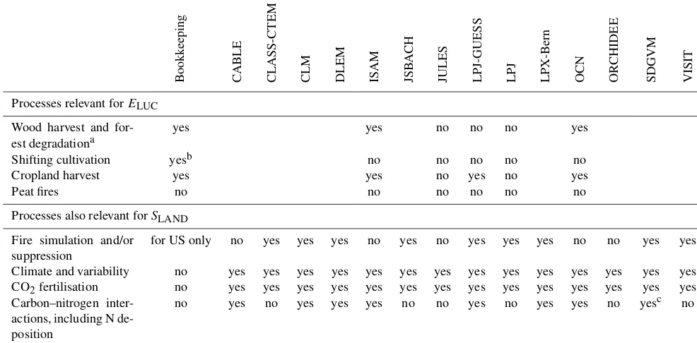
Table 5.Comparison of the processes included in the bookkeeping method and DGVMs in their estimates ofELUCandSLAND. See Table 6
for model references. All models include deforestation and forest regrowth after abandonment of agriculture (or from afforestation activities on agricultural land). Processes relevant forELUCare only described for the DGVMs used with land-cover change in this study (Fig. 6 top
panel).
Bookk
eeping
CABLE CLASS-CTEM CLM DLEM ISAM JSB
A
CH
JULES LPJ-GUESS LPJ LPX-Bern OCN ORCHIDEE SDGVM VISIT
Processes relevant forELUC
Wood harvest and for-est degradationa
yes yes no no no yes
Shifting cultivation yesb no no no no no
Cropland harvest yes yes no yes no yes
Peat fires no no no no no no
Processes also relevant forSLAND
Fire simulation and/or suppression
for US only no yes yes yes no yes no yes yes yes no no yes yes
Climate and variability no yes yes yes yes yes yes yes yes yes yes yes yes yes yes
CO2fertilisation no yes yes yes yes yes yes yes yes yes yes yes yes yes yes
Carbon–nitrogen inter-actions, including N de-position
no yes no yes yes yes no no yes no yes yes no yesc no
aRefers to the routine harvest of established managed forests rather than pools of harvested products.bNot in the recent update (Houghton and Nassikas, 2016).cVery
limited. Nitrogen uptake is simulated as a function of soil C, and Vcmax is an empirical function of canopy N. Does not consider N deposition.
on annual, national changes in cropland and pasture areas reported by the FAO Statistics Division (FAOSTAT, 2010). Land-use-change country data are aggregated by regions. The carbon stocks on land (biomass and soils), and their re-sponse functions subsequent to land-use change, are based on FAO data averages per land-cover type, per biome, and per region. Similar results were obtained using forest biomass carbon density based on satellite data (Baccini et al., 2012). The bookkeeping method does not include land ecosys-tems’ transient response to changes in climate, atmospheric CO2, and other environmental factors, and the growth/decay
curves are based on contemporary data that will implicitly reflect the effects of CO2and climate at that time. Published
results from the bookkeeping method are available from 1850 to 2010, with preliminary results available to 2015.
2.2.2 Fire-based interannual variability inELUC
CO2 emissions associated with land-use change calculated
from satellite-based fire activity in tropical forest areas (van der Werf et al., 2010) provide information on emissions due to tropical deforestation and degradation that are comple-mentary to the bookkeeping approach. They do not pro-vide a direct estimate ofELUCas they do not include
non-combustion processes such as respiration, wood harvest, wood products, or forest regrowth. Legacy emissions such
as decomposition from on-ground debris and soils are not included in this method either. However, fire estimates pro-vide some insight in the year-to-year variations in the sub-component of the totalELUC flux that result from
immedi-ate CO2emissions during deforestation caused, for example,
by the interactions between climate and human activity (e.g. there is more burning and clearing of forests in dry years) that are not represented by other methods. The “deforesta-tion fire emissions” assume an important role of fire in re-moving biomass in the deforestation process and thus can be used to infer gross instantaneous CO2emissions from
defor-estation using satellite-derived data on fire activity in regions with active deforestation. The method requires information on the fraction of total area burned associated with defor-estation vs. other types of fires, and this information can be merged with information on biomass stocks and the fraction of the biomass lost in a deforestation fire to estimate CO2
emissions. The satellite-based deforestation fire emissions are limited to the tropics, where fires result mainly from hu-man activities. Tropical deforestation is the largest and most variable single contributor toELUC.
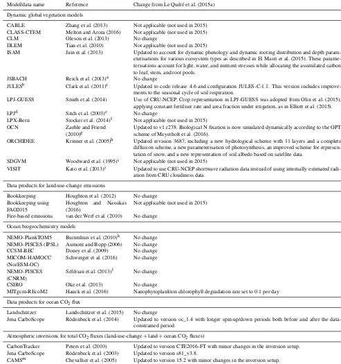
Table 6.References for the process models and data products included in Figs. 6–8. All models and products are updated with new data to end of year 2015.
Model/data name Reference Change from Le Quéré et al. (2015a) Dynamic global vegetation models
CABLE Zhang et al. (2013) Not applicable (not used in 2015) CLASS-CTEM Melton and Arora (2016) Not applicable (not used in 2015) CLM Oleson et al. (2013) No change
DLEM Tian et al. (2010) Not applicable (not used in 2015)
ISAM Jain et al. (2013) Updated to account for dynamic phenology and dynamic rooting distribution and depth param-eterisations for various ecosystem types as described in El Masri et al. (2015). These parame-terisations account for light, water, and nutrient stresses while allocating the assimilated carbon to leaf, stem, and root pools.
JSBACH Reick et al. (2013)a No change
JULESb Clark et al. (2011)c Updated to code release 4.6 and configuration JULES-C-1.1. This version includes improve-ments to the seasonal cycle of soil respiration.
LPJ-GUESS Smith et al. (2014) Use of CRU-NCEP. Crop representation in LPJ-GUESS was adopted from Olin et al. (2015), applying constant fertiliser rate and area fraction under irrigation, as in Elliott et al. (2015). LPJd Sitch et al. (2003)e No change
LPX-Bern Stocker et al. (2014)f Not applicable (not used in 2015) OCN Zaehle and Friend
(2010)g
Updated to v1.r278. Biological N fixation is now simulated dynamically according to the OPT scheme of Meyerholt et al. (2016).
ORCHIDEE Krinner et al. (2005)h Updated revision 3687, including a new hydrological scheme with 11 layers and a complete diffusion scheme, a new parameterisation of photosynthesis, an improved scheme for represen-tation of snow, and a new represenrepresen-tation of soil albedo based on satellite data.
SDGVM Woodward et al. (1995)i Not applicable (not used in 2015)
VISIT Kato et al. (2013)j Updated to use CRU-NCEP shortwave radiation data instead of using internally estimated radi-ation from CRU cloudiness data.
Data products for land-use-change emissions
Bookkeeping Houghton et al. (2012) No change Bookkeeping using
FAO2015
Houghton and Nassikas (2016)
Not applicable (not used in 2015) Fire-based emissions van der Werf et al. (2010) No change
Ocean biogeochemistry models
NEMO-PlankTOM5 Buitenhuis et al. (2010)k No change NEMO-PISCES (IPSL) Aumont and Bopp (2006) No change CCSM-BEC Doney et al. (2009) No change MICOM-HAMOCC
(NorESM-OC)
Schwinger et al. (2016) No change NEMO-PISCES
(CNRM)
Séférian et al. (2013)l No change CSIRO Oke et al. (2013) No change
MITgcm-REcoM2 Hauck et al. (2016) Nanophytoplankton chlorophyll degradation rate set to 0.1 per day Data products for ocean CO2flux
Landschützer Landschützer et al. (2015) No change
Jena CarboScope Rödenbeck et al. (2014) Updated to version oc_1.4 with longer spin-up/down periods both before and after the data-constrained period.
Atmospheric inversions for total CO2fluxes (land-use-change+land+ocean CO2fluxes)
CarbonTracker Peters et al. (2010) Updated to version CTE2016-FT with minor changes in the inversion setup. Jena CarboScope Rödenbeck et al. (2003) Updated to version s81_v3.8.
CAMSm Chevallier et al. (2005) Updated to version 15.2 with minor changes in the inversion setup.
aSee also Goll et al. (2015).bJoint UK Land Environment Simulator.cSee also Best et al. (2011).dLund–Potsdam–Jena.eCompared to published version, decreased LPJ wood harvest efficiency so
that 50 % of biomass was removed off-site compared to 85 % used in the 2012 budget. Residue management of managed grasslands increased so that 100 % of harvested grass enters the litter pool.
fCompared to published version: changed several model parameters, due to new tuning with multiple observational constraints. No mechanistic changes.gSee also Zaehle et al. (2011).hCompared to
published version: revised parameters values for photosynthetic capacity for boreal forests (following assimilation of FLUXNET data), updated parameters values for stem allocation, maintenance respiration and biomass export for tropical forests (based on literature), and CO2down-regulation process added to photosynthesis.iSee also Woodward and Lomas (2004). Changes from publications
include sub-daily light downscaling for calculation of photosynthesis and other adjustments.jSee also Ito and Inatomi (2012).kWith no nutrient restoring below the mixed layer depth.lUses winds from Atlas et al. (2011).mThe CAMS (Copernicus Atmosphere Monitoring Service) v15.2 CO2inversion system, initially described by Chevallier et al. (2005), relies on the global tracer transport
fires that are detected by satellite as thermal anomalies but not mapped by the burned-area approach (Randerson et al., 2012). The burned-area information is used as input data in a modified version of the satellite-driven Carnegie–Ames– Stanford Approach (CASA) biogeochemical model to esti-mate carbon emissions associated with fires, keeping track of what fraction of fire emissions was due to deforestation (see van der Werf et al., 2010). The CASA model uses differ-ent assumptions to compute decay functions compared to the bookkeeping method, and does not include historical emis-sions or regrowth from land-use change prior to the avail-ability of satellite data. Comparing coincident CO emissions and their atmospheric fate with satellite-derived CO concen-trations allows for some validation of this approach (e.g. van der Werf et al., 2008). Results from the fire-based method to estimate land-use-change emissions anomalies added to the bookkeeping mean ELUC estimate are available from 1997 to 2015. Our combination of land-use-change CO2emissions
where the variability in annual CO2deforestation emissions
is diagnosed from fires assumes that year-to-year variability is dominated by variability in deforestation.
2.2.3 Dynamic global vegetation models (DGVMs)
Land-use-change CO2emissions have been estimated using
an ensemble of DGVM simulations. New model experiments up to year 2015 have been coordinated by the project “Trends and drivers of the regional-scale sources and sinks of carbon dioxide” (TRENDY; Sitch et al., 2015). We use only models that have estimated land-use-change CO2emissions
follow-ing the TRENDY protocol (see Sect. 2.5.2). Models use their latest configurations, summarised in Tables 5 and 6.
Two sets of simulations were performed with the DGVMs, first forced with historical changes in land-cover distribution, climate, atmospheric CO2concentration, and N deposition,
and second, as further described below with a time-invariant pre-industrial land-cover distribution, allowing for estima-tion of, by difference with the first simulaestima-tion, the dynamic evolution of biomass and soil carbon pools in response to prescribed land-cover change. Because of the limited avail-ability of the land-use forcing (see below), 14 DGVMs per-formed historical simulations with time-invariant land-cover distribution, but only 5 DGVMs managed to simulate realis-tic simulations with time varying land-cover change. These latter DGVMs accounted for deforestation and (to some ex-tent) regrowth, the most important components ofELUC, but they do not represent all processes resulting directly from human activities on land (Table 5). All DGVMs represent processes of vegetation growth and mortality, as well as de-composition of dead organic matter associated with natural cycles, and include the vegetation and soil carbon response to increasing atmospheric CO2levels and to climate
variabil-ity and change. In addition, eight models explicitly simulate the coupling of C and N cycles and account for atmospheric N deposition (Table 5), with three of those models used for
land-use-change simulations. The DGVMs are independent of the other budget terms except for their use of atmospheric CO2concentration to calculate the fertilisation effect of CO2
on primary production.
For this global carbon budget, the DGVMs used the HYDE land-use-change data set (Klein Goldewijk et al., 2011), which provides annual, half-degree, fractional data on cropland and pasture. These data are based on annual FAO statistics of change in agricultural area available to 2012 (FAOSTAT, 2010). For the years 2013 to 2015, the HYDE data were extrapolated by country for pastures and cropland separately based on the trend in agricultural area over the pre-vious 5 years. The more comprehensive harmonised land-use data set (Hurtt et al., 2011), which also includes fractional data on primary vegetation and secondary vegetation, as well as all underlying transitions between land-use states, has not been made available yet for this year. Hence, the reduced en-semble of DGVMs that can simulate the LUC flux from the HYDE data set only. The HYDE data are independent of the data set used in the bookkeeping method (Houghton, 2003, and updates), which is based primarily on forest area change statistics (FAO, 2010). The HYDE land-use-change data set does not indicate whether land-use changes occur on forested or non-forested land; it only provides the changes in agri-cultural areas. Hence, it is implemented differently within each model (e.g. an increased cropland fraction in a grid cell can be at the expense of either grassland or forest, the latter resulting in deforestation; land-cover fractions of the non-agricultural land differ between models). Thus, the DGVM forest area and forest area change over time is not consis-tent with the Forest Resource Assessment of the FAO forest area data used for the bookkeeping model to calculateELUC. Similarly, model-specific assumptions are applied to convert deforested biomass or deforested area, and other forest prod-uct pools, into carbon in some models (Table 5).
The DGVM runs were forced by either 6-hourly CRU-NCEP or by monthly CRU temperature, precipitation, and cloud cover fields (transformed into incoming surface radi-ation) based on observations and provided on a 0.5◦×0.5◦ grid and updated to 2015 (Harris et al., 2014; Viovy, 2016). The forcing data include both gridded observations of cli-mate and global atmospheric CO2, which change over time
(Dlugokencky and Tans, 2016), and N deposition (as used in some models; Table 5). As mentioned before,ELUCis di-agnosed in each model by the difference between a model simulation with prescribed historical land-cover change and a simulation with constant, pre-industrial land-cover distribu-tion. Both simulations were driven by changing atmospheric CO2, climate, and, in some models, N deposition over the
period 1860–2015. Using the difference between these two DGVM simulations to diagnose ELUC is not fully
consis-tent with the definition ofELUCin the bookkeeping method
(Gasser and Ciais, 2013; Stocker and Joos, 2015). The DGVM approach to diagnose land-use-change CO2
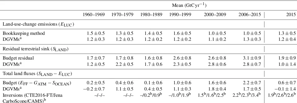
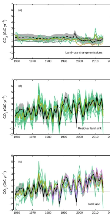
Table 7.Comparison of results from the bookkeeping method and budget residuals with results from the DGVMs and inverse estimates for the periods 1960–1969, 1970–1979, 1980–1989, 1990–1999, and 2000–2009, as well as the last decade and last year available. All values are in GtC yr−1. The DGVM uncertainties represent±1σof the decadal or annual (for 2015 only) estimates from the individual models; for the inverse models all three results are given where available.
Mean (GtC yr−1)
1960–1969 1970–1979 1980–1989 1990–1999 2000–2009 2006–2015 2015
Land-use-change emissions (ELUC)
Bookkeeping method 1.5±0.5 1.3±0.5 1.4±0.5 1.6±0.5 1.0±0.5 1.0±0.5 1.3±0.5
DGVMsa 1.2±0.3 1.2±0.3 1.2±0.2 1.2±0.2 1.1±0.2 1.3±0.3 1.2±0.4
Residual terrestrial sink (SLAND)
Budget residual 1.7±0.7 1.7±0.8 1.6±0.8 2.6±0.8 2.6±0.8 3.1±0.9 1.9±0.9
DGVMsa 1.2±0.5 2.2±0.5 1.7±0.6 2.3±0.5 2.8±0.6 2.8±0.7 1.0±1.4
Total land fluxes (SLAND−ELUC)
Budget (EFF−GATM−SOCEAN) 0.2±0.5 0.4±0.6 0.1±0.6 1.0±0.6 1.6±0.6 2.2±0.7 0.6±0.7
DGVMsa −0.2±0.7 1.1±0.5 0.4±0.5 1.1±0.3 1.8±0.4 1.7±0.5 −0.1±1.4
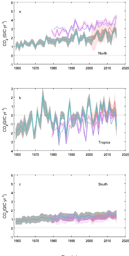
Inversions (CTE2016-FT/Jena CarboScope/CAMS)b
–/–/– –/–/– –/0.2b/0.9b –/1.0b/1.9b 1.5b/1.6b/2.5b 2.2b/2.3b/3.4b 1.9b/2.6b/2.6b
aNote that for DGVMs, the mean reported for the total land fluxes is not equal to the difference between the means reported forS
LANDandELUCas a different set of models contributed to these two estimates (see Sect. 2.2.3).bEstimates are not corrected for the influence of river fluxes, which would reduce the fluxes by 0.45 GtC yr−1when neglecting the anthropogenic influence on land (Sect. 2.7.2). See Table 6 for model references.
ELUCemissions than the bookkeeping approach if all the pa-rameters of the two approaches were the same, which is not the case (see Sect. 2.5.2).
2.2.4 Uncertainty assessment forELUC
Differences between the bookkeeping, the addition of fire-based interannual variability to the bookkeeping, and DGVM methods originate from three main sources: the land-cover-change data set, the different approaches used in models, and the different processes represented (Table 5). We examine the results from the DGVMs and of the bookkeeping method to assess the uncertainty inELUC.
The uncertainties in annualELUCestimates are examined
using the standard deviation across models, which averages 0.3 GtC yr−1from 1959 to 2015 (Table 7). The mean of the multi-modelELUCestimates is consistent with a combination
of the bookkeeping method and fire-based emissions (Ta-ble 7), with the multi-model mean and bookkeeping method differing by less than 0.5 GtC yr−1 over 85 % of the time. Based on this comparison, we determine that an uncertainty of ±0.5 GtC yr−1 provides a semi-quantitative measure of uncertainty for annual emissions and reflects our best value judgement that there is at least 68 % chance (±1σ) that the true land-use-change emission lies within the given range, for the range of processes considered here. This is consis-tent with the uncertainty analysis of Houghton et al. (2012), which partly reflects improvements in data on forest area change using data and partly more complete understanding and representation of processes in models.
The uncertainties in the decadalELUCestimates are also
examined using the DGVM ensemble, although they are
likely correlated between decades. The correlations between decades come from (1) common biases in system bound-aries (e.g. not counting forest degradation in some models), (2) common definition for the calculation ofELUCfrom the difference of simulations with and without land-use change (a source of bias vs. the unknown truth), (3) common and uncertain land-cover change input data which also cause a bias (though if a different input data set is used each decade, decadal fluxes from DGVMs may be partly decorrelated), and (4) model structural errors (e.g. systematic errors in biomass stocks). In addition, errors arising from uncertain DGVM parameter values would be random but they are not accounted for in this study, since no DGVM provided an en-semble of runs with perturbed parameters.
Prior to 1959, the uncertainty inELUCis taken as±33 %, which is the ratio of uncertainty to mean from the 1960s in the bookkeeping method (Table 7), the first decade avail-able. This ratio is consistent with the mean standard devia-tion of DGVMs land-use-change emissions over 1870–1958 (0.32 GtC) over the multi-model mean (0.9 GtC).
2.3 Growth rate in atmospheric CO2 concentration (GATM)
Global growth rate in atmospheric CO2concentration
The rate of growth of the atmospheric CO2