www.geosci-model-dev.net/9/1341/2016/ doi:10.5194/gmd-9-1341-2016
© Author(s) 2016. CC Attribution 3.0 License.
TerrSysMP–PDAF (version 1.0): a modular high-performance data
assimilation framework for an integrated land
surface–subsurface model
Wolfgang Kurtz1,2, Guowei He1,2, Stefan J. Kollet1,2, Reed M. Maxwell3, Harry Vereecken1,2, and Harrie-Jan Hendricks Franssen1,2
1Forschungszentrum Jülich GmbH, Institute of Bio- and Geosciences, IBG-3 (Agrosphere), Jülich, Germany 2Centre for High-Performance Scientific Computing in Terrestrial Systems (HPSC-TerrSys), Geoverbund ABC/J, Jülich, Germany
3Department of Geology and Geological Engineering and Integrated Groundwater Modeling Center, Colorado School of Mines, Golden, CO, USA
Correspondence to: Wolfgang Kurtz ([email protected])
Received: 14 September 2015 – Published in Geosci. Model Dev. Discuss.: 3 November 2015 Revised: 24 March 2016 – Accepted: 29 March 2016 – Published: 11 April 2016
Abstract. Modelling of terrestrial systems is continuously moving towards more integrated modelling approaches, where different terrestrial compartment models are combined in order to realise a more sophisticated physical descrip-tion of water, energy and carbon fluxes across compartment boundaries and to provide a more integrated view on terres-trial processes. While such models can effectively reduce cer-tain parameterisation errors of single compartment models, model predictions are still prone to uncertainties regarding model input variables. The resulting uncertainties of model predictions can be effectively tackled by data assimilation techniques, which allow one to correct model predictions with observations taking into account both the model and measurement uncertainties. The steadily increasing availabil-ity of computational resources makes it now increasingly possible to perform data assimilation also for computation-ally highly demanding integrated terrestrial system models. However, as the computational burden for integrated models as well as data assimilation techniques is quite large, there is an increasing need to provide computationally efficient data assimilation frameworks for integrated models that al-low one to run on and to make efficient use of massively par-allel computational resources. In this paper we present a data assimilation framework for the land surface–subsurface part of the Terrestrial System Modelling Platform (TerrSysMP). TerrSysMP is connected via a memory-based coupling ap-proach with the pre-existing parallel data assimilation library
PDAF (Parallel Data Assimilation Framework). This frame-work provides a fully parallel modular environment for per-forming data assimilation for the land surface and the subsur-face compartment. A simple synthetic case study for a land surface–subsurface system (0.8 million unknowns) is used to demonstrate the effects of data assimilation in the inte-grated model TerrSysMP and to assess the scaling behaviour of the data assimilation system. Results show that data as-similation effectively corrects model states and parameters of the integrated model towards the reference values. Scal-ing tests provide evidence that the data assimilation system for TerrSysMP can make efficient use of parallel computa-tional resources for >30 k processors. Simulations with a large problem size (20 million unknowns) for the forward model were also efficiently handled by the data assimilation system. The proposed data assimilation framework is useful in simulating and estimating uncertainties in predicted states and fluxes of the terrestrial system over large spatial scales at high resolution utilising integrated models.
1 Introduction
forcing terms and model parameters, which are, for example, related to the spatial and temporal variability of certain model input like precipitation, soil hydraulic properties or vegeta-tion parameters. In addivegeta-tion, the determinavegeta-tion of adequate initial conditions for terrestrial system simulations is of-ten highly uncertain. Ensemble-based data assimilation (DA) techniques are gaining increasing attention in the geoscien-tific community as a tool to merge such uncertain model pre-dictions with uncertain observation data. These techniques follow a Monte Carlo approach in which an ensemble of dif-ferent model realisations is integrated forward in time. The different model realisations can include various uncertainties in the model input, which then allows one to approximate the variability of model predictions for different model state vari-ables given the different uncertainty sources. These uncertain model predictions are then sequentially conditioned to avail-able observation data where predictions and data are opti-mally combined according to their uncertainties. This results in updated model states, which are merged closer towards the measurements and provide an improved model forecast for the following time steps. Data assimilation has already been applied to a wide variety of models in different compart-ments of the terrestrial system, including atmosphere, land surface and groundwater using various kinds of observation data. In this overview we focus on the water and energy cy-cles of the terrestrial system. The most commonly applied data assimilation algorithm in such systems is the ensemble Kalman filter (EnKF) (Evensen, 1994; Burgers et al., 1998) and its deterministic variants (e.g. Anderson, 2001; Bishop et al., 2001; Tippett et al., 2003). In groundwater hydrology, usually pressure head data are assimilated (Chen and Zhang, 2006; Hendricks Franssen and Kinzelbach, 2008; Nowak, 2009) and to a lesser extend also transport-related data, like solute concentrations (Liu et al., 2008; Li et al., 2012), mo-lar fractions of chemical constituents (Gharamti et al., 2014) or groundwater temperatures (Kurtz et al., 2014). Data as-similation has also been applied for variably saturated condi-tions in synthetic model set-ups (e.g. Erdal et al., 2014; Song et al., 2014; L. Shi et al., 2015) as well as for real-world data (e.g. Li and Ren, 2011; Wu and Margulis, 2011, 2013). Typ-ically in these cases, point measurements of pressure or soil moisture are assimilated. Data assimilation techniques were also used in the context of coupled surface–subsurface flow (Camporese et al., 2009; Bailey and Baù, 2012; Rasmussen et al., 2015) where the focus is mostly on the assimilation of pressure head and discharge data. In land surface data assimilation the most commonly assimilated data types are remotely sensed soil moisture products or brightness tem-peratures (Crow and Wood, 2003; De Lannoy et al., 2007; Han et al., 2013) but also land surface temperature (Kumar and Kaleita, 2003; Ghent et al., 2010; Reichle et al., 2010; Han et al., 2013), snow cover data (Andreadis and Letten-maier, 2006; Su et al., 2010; Xu and Shu, 2014) or leaf area index (Sabater et al., 2008; Ford and Quiring, 2013; Barbu et al., 2014). The assimilation of such observation data into
either land surface or subsurface models usually leads to an improvement of the predictive capability of the respec-tive model. Besides the correction of model state variables, it has become common especially in subsurface and land surface data assimilation to also correct model parameters jointly with model states. The reason is that the parametric uncertainty in such models is rather high compared to other compartments, like the atmosphere, where initial value prob-lems dominate the uncertainty. Examples for the joint cor-rection of model states and parameters in land surface and subsurface models are the correction of hydraulic subsurface parameters like hydraulic conductivity (Chen and Zhang, 2006; Hendricks Franssen and Kinzelbach, 2008; Rasmussen et al., 2015; Pasetto et al., 2015), porosity (Li et al., 2012, 2015), leakage coefficients (Kurtz et al., 2013; Rasmussen et al., 2015), van Genuchten parameters (Li and Ren, 2011; Montzka et al., 2011; Y. Shi et al., 2014; L. Shi et al., 2015), dispersion parameters (Li et al., 2015) or textural informa-tion (Han et al., 2014). Other examples in the context of land surface modelling include the estimation of vegetation pa-rameters like stomatal resistance and canopy water storage (Y. Shi et al., 2015) or the estimation of parameters related to land surface flux partitioning (Bateni and Entekhabi, 2012). In most cases, this joint updating of model states and model parameters leads to better simulation results than a correction of model states alone because the uncertainties coming from a wrong parameterisation are reduced.
ground-water and a regional climate model leads to different pre-cipitation and evapotranspiration estimates compared to the stand alone regional climate model especially during sum-mer time. Maxwell et al. (2011), Shrestha et al. (2014) and Rahman et al. (2015) provided further examples how sub-surface dynamics affect the development of the atmospheric boundary layer.
Due to these various feedbacks, there is a growing num-ber of modelling platforms that integrate different com-partment models for subsurface, land surface and atmo-sphere, e.g. ParFlow-CLM (Maxwell and Miller, 2005; Kol-let and Maxwell, 2008), ParFlow-WRF (Maxwell et al., 2011), COSMO-CLM2 (Davin et al., 2011), AquiferFlow-SiB2 (Tian et al., 2012), Terrestrial System Modelling Plat-form (TerrSysMP) (Shrestha et al., 2014) or HIRHAM-MIKESHE (Butts et al., 2014). Such models allow for a more integrated view of the terrestrial system and water cycle in particular and the coupling leads to a physically more con-sistent description of processes across compartment scales. However, while such integrated modelling approaches pro-vide a better description of model physics, which effectively reduces model structural errors that often occur in single compartment models through the parameterisation of lower or upper boundary conditions, the parameter and forcing un-certainty still remains in such models. Therefore, data assim-ilation methods may also help to quantify the uncertainties of integrated modelling approaches and to improve their fore-cast capability through the merging with observation data. Integrated models are usually computationally expensive and often need to be run on a high-performance computational infrastructure. Therefore, there is a need to establish data as-similation frameworks that can efficiently cope with the high computational burden of integrated terrestrial system models. This is especially relevant when simulations are performed at a high spatial resolution and when a relatively high number of model realisations are needed, which is typically the case for ensemble-based data assimilation with land surface and subsurface models.
A number of frameworks exist that can be used to per-form data assimilation for specific Earth system components. Land surface examples include the Canadian Land Data As-similation System (CaLDAS) (Carrera et al., 2015) or the Global Land Data Assimilation System (GLDAS) (Rodell et al., 2004). An example for an atmospheric data assimi-lation system is provided by Barker et al. (2012) who devel-oped this system for the numerical weather prediction model WRF (WRFDA). Ridler et al. (2014) developed an assimi-lation system for the hydrological model MIKE SHE. How-ever, these data assimilation systems usually rely on a sim-plified representation of groundwater dynamics because the process description in most land surface models does not in-clude lateral flows and surface water–groundwater interac-tions. Additionally, most data assimilation frameworks are unable to perform joint state–parameter estimation, which has been shown to be important in the context of subsurface
and land surface data assimilation. An exception is the data assimilation system for the groundwater model MIKE SHE, which includes lateral groundwater flow and surface water– groundwater exchange and also allows for a joint update of states and model parameters. However, unsaturated flow in MIKE SHE is still only calculated in 1-D.
Besides the above-mentioned data assimilation systems for certain Earth system compartments, there are also a num-ber of generic data assimilation frameworks, which are not tailored to a specific simulation model. Examples of such generic data assimilation frameworks are the Data Assimi-lation Research Testbed (DART) (Anderson et al., 2009), the Parallel Data Assimilation Framework (PDAF) (Nerger and Hiller, 2013) or the OpenDA framework (OpenDA, 2013). These different frameworks provide various data assimila-tion algorithms and the necessary computaassimila-tional infrastruc-ture to operate with any kind of simulation model. Ridler et al. (2014) demonstrated the use of the OpenDA framework to establish a data assimilation system for the hydrological model MIKE SHE. This was achieved by connecting both components with the Open Modelling Interface (OpenMI) software. This kind of interfacing is based on Java and .NET technology and can also be used for other OpenMI compli-ant models. However, the utilised communication approach between model and data assimilation may not be efficient enough to be applied for large data assimilation problems.
assimi-lation framework for a simple land surface–subsurface set-up with a focus on hydrological model states and fluxes. In this section also the scaling behaviour of the data assim-ilation framework and its applicability for high-resolution modelling problems is tested and presented in detail. Finally, Sect. 6 provides conclusions and an outlook on possible fur-ther developments.
2 Terrestrial System Modelling Platform
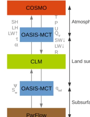
The recently developed TerrSysMP (Shrestha et al., 2014) is a modular scale-consistent terrestrial system model consist-ing of three already well-established models for the atmo-sphere, the land surface and the subsurface (see Fig. 1).
Atmospheric processes are simulated with COSMO-DE (Baldauf et al., 2011), which is the operational forecast model of the German weather service. COSMO-DE is con-vection permitting and utilises a terrain-following coordinate system with variable vertical layer thickness. For more de-tails on the model physics see Shrestha et al. (2014).
The land surface part of TerrSysMP consists of the CLM version 3.5 (Oleson et al., 2004, 2008). CLM calculates the transfer of energy, momentum and carbon between the surface, vegetation and the atmosphere. In CLM, the sub-surface is represented with 10 soil layers of variable thick-ness with a total extent of 3 m. Soil water and soil temper-ature dynamics are calculated only in a vertical direction; i.e. there is no lateral exchange between grid cells. Snow accumulation is represented with up to five snow layers on top of the soil layer. Vegetation is parameterised with up to 16 plant functional types providing the plant physiological parameters that are used to calculate the contribution of veg-etation to radiative transfer, land surface fluxes and carbon dynamics. CLM provides prognostic variables for the sub-surface (soil moisture, soil temperature, groundwater stor-age), surface water routing, land surface fluxes (evaporation from ground and vegetation, transpiration from vegetation, sensible heat fluxes from ground and vegetation), radiative transfer (adsorption/transmittance of solar radiation, adsorp-tion/emission of short-wave radiation) and carbon fluxes.
The subsurface part of TerrSysMP consists of the vari-ably saturated finite-difference groundwater model ParFlow (Ashby and Falgout, 1996; Jones and Woodward, 2001; Kol-let and Maxwell, 2006; Maxwell, 2013). ParFlow solves the 3-D Richards equation and includes a surface water routing scheme, which is based on the kinematic wave approxima-tion of overland flow coupling subsurface and overland flow in an integrated fashion (Kollet and Maxwell, 2006). The sys-tem of partial differential equations is solved with a Newton– Krylow method (Jones and Woodward, 2001). Additionally, ParFlow provides a terrain-following grid transform with variable vertical discretisation (Maxwell, 2013), which al-lows it to solve groundwater problems with high topographic gradients.
Figure 1. Coupling of the TerrSysMP component models ParFlow (subsurface), CLM (land surface) and COSMO-DE (atmosphere) by OASIS-MCT. The exchanged fluxes and state variables are:ψ
(subsurface pressure),Sw(subsurface saturation),qinf(net infiltra-tion flux), SH (sensible heat flux), LH (latent heat flux), LW↑ (out-going long-wave radiation),τ(momentum flux),α(albedo),P (air pressure),T (air temperature),U(wind velocity), SW↓(incoming short-wave radiation), LW↓(incoming long-wave radiation),QV (specific humidity) andR(precipitation).
CLM with its calculated subsurface pressure (ψ) and satura-tion (Sw) values for the first 10 subsurface layers and in return CLM provides the upper boundary condition for ParFlow, consisting of the recharge values (qinf) that are calculated based on the land surface fluxes of CLM (precipitation, in-terception, total evaporation, total transpiration). In the land surface–atmosphere part of TerrSysMP, CLM provides land surface fluxes (sensible heat flux SH and latent heat flux LH), outgoing long-wave radiation (LW↑), momentum flux (τ) and albedo (α) as a lower boundary condition to COSMO-DE. In turn, COSMO-DE provides forcing data to CLM in-cluding air pressure (P), air temperature (T), wind velocity (U), incoming short-wave (SW) and long-wave (LW↓) radi-ation, specific humidity (QV) and precipitation (R).
The advantages of this integrated modelling approach with TerrSysMP are twofold:
1. The coupling of the different component models im-proves the physical representation especially at the in-terfaces of the different geoscientific compartments. For example, ParFlow replaces the simplified soil hydrol-ogy (1-D only) and surface water routing (uncoupled) schemes in CLM by a fully integrated 3-D variably sat-urated surface–subsurface flow model. In COSMO the simplified land surface scheme TERRA is replaced with the more sophisticated land surface scheme of CLM, for example, concerning the representation of vegetation. 2. This modelling approach allows for an integrated view
of the terrestrial water, energy and carbon cycles be-cause the dynamic feedbacks of the different geoscien-tific compartments are explicitly taken into account. Another interesting feature of TerrSysMP is its modular-ity: apart from the fully coupled system (ParFlow, CLM and COSMO-DE) it is also possible to compile and run only the land surface–subsurface part (CLM and ParFlow) or the land surface–atmosphere part (CLM and COSMO-DE) or each of the component models individually. Regarding the paral-lel performance, TerrSysMP has already shown to be highly scalable on the massively parallel supercomputing environ-ment JUQUEEN (Jülich BlueGene/Q) (Gasper et al., 2014).
3 Parallel Data Assimilation Framework
The PDAF library (Nerger and Hiller, 2013) provides a generic framework for applying data assimilation with any kind of geoscientific model. PDAF provides parallel algo-rithms of already well-established data assimilation meth-ods like the ensemble Kalman filter (Evensen, 1994; Burgers et al., 1998) or the local ensemble transform Kalman filter (LETKF) (Hunt et al., 2007). Furthermore, PDAF provides the user with generic routines to interface the model with the data assimilation algorithms and it includes methods for establishing the parallel communication for the model and
the data assimilation algorithms. The data transfer (coupling) between the model and the data assimilation module can be handled in two ways:
– offline coupling: data exchange via the input/output files of the model;
– online coupling: data exchange via main memory. The first method (offline coupling) is more ad hoc and also applicable when the source code of the model is not avail-able. In this case, the user needs to take care of the execution of the model forward runs to the next assimilation cycle. An additional executable containing calls to PDAF routines is then used to perform the data assimilation. Within this ex-ecutable, PDAF reads the state vector from the model out-put files, performs the assimilation and writes out the assim-ilation results in the form of input files for the next model integration. One drawback is that this coupling method pro-duces a lot of I/O overhead because a huge number of files has to be read and written at each assimilation step. Another drawback of the offline coupling is that the model needs to be re-initialised after each assimilation step. In the second variant (online coupling), PDAF is directly integrated into the model source code. This enables a direct data transfer between the model and the data assimilation algorithms of PDAF via main memory. Additionally, the model only needs to be initialised once because the model integration is only paused for the data assimilation with PDAF within the time stepping loop of the model. This coupling variant is signif-icantly faster in terms of CPU time but requires more pro-gramming effort and the availability of the model source code.
The model coupling for both coupling variants (offline and online) is defined by the user through the aforementioned generic interface routines that are provided by PDAF. These routines include
– The definition of the state vector for PDAF, which has to be provided by the model either from the model output files or via exchange in main memory.
– The definition of the measurement vector and the cor-responding measurement uncertainties and error covari-ances (usually via observation files).
– Rules on how the updated state vector is transferred back to the model.
the application and several interface routines are provided by PDAF to construct this matrix.
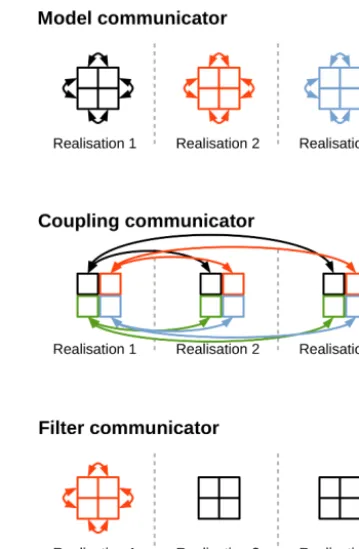
At the very beginning of the initialisation phase of the model, a PDAF routine needs to be called that establishes the parallel communication within the model and the data assim-ilation algorithms. This is especially important for fully par-allel models like the ones in TerrSysMP. In this phase, PDAF creates three parallel communicators: the model communi-cator, the coupling communicator and the filter communica-tor. The general layout of these communicators is depicted in Fig. 2 for a model set-up with three ensemble members and four processors per model realisation. The model communi-cator is created for each ensemble member separately and in the case of a parallel model it is equal to the models’ internal communicator (i.e. a replacement of MPI_COMM_WORLD). The filter communicator is used to perform the filter algo-rithms that are only applied on the processors of the first en-semble member (marked in red colour in Fig. 2), while the other processors remain idle during the filter update. Within the filter communicator, the processors exchange information about the simulation results at observation points and global ensemble statistics (ensemble mean and variance). The cou-pling communicator is the communicator for exchanging data between the processors in the filter communicator and the remaining ensemble members before and after the assim-ilation step. As noted by the arrows in Fig. 2, this data ex-change is according to the processor ranks in the model com-municator; i.e. the data exchange only takes place for each subdomain of the model and not on a global level. A global vector of model states is never used in this scheme.
4 TerrSysMP–PDAF
This section describes the implementation and usage of the data assimilation system for TerrSysMP, which is referred to as TerrSysMP–PDAF in the following.
4.1 Technical implementation
In order to establish a data assimilation system for the land surface–subsurface part of TerrSysMP (CLM and ParFlow) with the data assimilation framework PDAF, an interface be-tween the model and the data assimilation framework was created. As the forward model is already computationally very demanding and the source code of the model is read-ily available, we decided to follow the online coupling ap-proach (data exchange via main memory and not running the model as a single executable) in order to avoid frequent re-initialisations of the model and a significant overhead in I/O operations both of which degrade the performance of the constructed data assimilation system for TerrSysMP. In or-der to accomplish this, several changes in the source code and the building script of TerrSysMP had to be undertaken. First, the main program sections of the two component
mod-Figure 2. Communicators in PDAF for a parallel set-up with three ensemble members and four processors per ensemble member. Colours indicate the membership of the respective processors and arrows exemplify the parallel communication between the different processors.
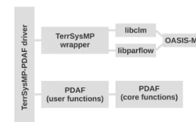
the model source code (and building procedure), it was pos-sible to combine the model libraries for CLM and ParFlow (including OASIS-MCT) with the data assimilation libraries provided by PDAF in one main program. Figure 3 sketches the different components of the TerrSysMP–PDAF frame-work. The TerrSysMP–PDAF driver (i.e. the main program) controls the whole framework. This includes the initialisa-tion and finalisainitialisa-tion of MPI, TerrSysMP and PDAF as well as the time stepping control for the model forward integration and the data assimilation. The TerrSysMP wrapper is used to interface the driver program with the individual model libraries (libclm and libparflow coupled via OASIS-MCT). The PDAF user(-defined) functions are specifically adapted to TerrSysMP and the desired assimilation scheme (EnKF in this case) and include, for example, the definition of the state vector, the observation vector and the observation error co-variance matrix. These data are either provided by the model directly (e.g. state vector) or are read from files or command line options (e.g. observations and observation errors). The PDAF core functions provide the algorithms for different fil-tering methods. This part of PDAF is not modified for the implementation of TerrSysMP–PDAF because the input for the PDAF core functions (e.g. state vector, observation vec-tor, observation error covariance matrix) is already provided by the PDAF user functions.
The TerrSysMP–PDAF driver program proceeds in the fol-lowing steps:
1. initialisation of MPI;
2. initialisation of the parallel communication by PDAF; 3. model initialisation for CLM and ParFlow;
4. initialisation of data structures in PDAF (state vector, measurement vector, etc.);
5. time loop over measurement time steps:
a. advance CLM and ParFlow to the next assimilation time step;
b. filter step by PDAF;
c. update of the relevant model variables in CLM and ParFlow;
6. finalisation of PDAF, CLM and ParFlow.
In steps 1 and 2, the global MPI communicator as well as the PDAF communicators (see Sect. 3 and Fig. 2) are ini-tialised. In step 3, all processors first read a common input file, which holds information about specific settings for the data assimilation run. This includes the number of processors for CLM and ParFlow for each model realisation, the num-ber of ensemble memnum-bers, time stepping information, speci-fication of the observation data and the model variables that should be updated as well as settings for the model output. Then, within each realisation (model communicator) each
Figure 3. Components of TerrSysMP–PDAF.
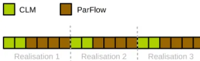
Figure 4. Example of the processor layout of TerrSysMP–PDAF for three model realisations where each realisations is simulated with two processors for CLM and four processors for ParFlow.
results at observation locations from the state vector. Note that by using grid cell indices, no interpolation or other kind of measurement operation is performed because the observa-tions are simply clipped to the nearest model grid cell. The measurement covariance matrix in the current implementa-tion is always diagonal (i.e. the measurement errors for the different observations are uncorrelated) and the measurement error can be different for the individual observations. After-wards, the filter update is performed. The choice of the data assimilation algorithm for TerrSysMP is currently restricted to the ensemble Kalman filter. After the filtering step, the up-dated state vector is transferred back to the corresponding model variables in step 5c and TerrSysMP–PDAF proceeds to the next assimilation cycle. When all assimilation cycles are finished, the data structures of the individual components of TerrSysMP–PDAF are deallocated in step 6 and the pro-gram is shut down.
Time stepping for the TerrSysMP component models as well as in the data assimilation loop is static; i.e. there is a constant time step for the model integration of TerrSysMP and a constant frequency for the assimilation steps, which is a multiple of the TerrSysMP time step.
As TerrSysMP is designed in a modular fashion, the same approach was also chosen for the data assimilation system for the land surface–subsurface part of TerrSysMP. That is, the data assimilation system can run only with ParFlow, only with CLM or for CLM and ParFlow coupled with OASIS-MCT. In the case of using a single model of TerrSysMP, the aforementioned changes of OASIS-MCT communicators for allowing an ensemble propagation are not applicable any more. Instead, the model communicator of PDAF is directly transferred to the internal model communicators of CLM or ParFlow.
In the coupled (ParFlow+CLM) and uncoupled (ParFlow stand alone) TerrSysMP configuration, measurements of pressure or soil moisture can be assimilated in ParFlow. The assimilation of both measurement types involves an update of pressure values in ParFlow because this is ParFlow’s prog-nostic variable and soil moisture (or saturation) is a derived quantity, which is not directly used as a state variable for the next time step. For the assimilation of pressure data, sim-ulated pressure values in ParFlow are directly modified by the pressure observations. For the assimilation of soil mois-ture data, two options are implemented in TerrSysMP–PDAF
to update pressure values with soil moisture observations: (1) the state vector consists of soil moisture and pressure values of ParFlow. In this case, pressure values in ParFlow are indirectly corrected with the incoming soil moisture mea-surements through the correlations between soil moisture and pressure. (2) The state vector solely contains soil moisture values and the updated soil moisture values are transformed back to pressure values via the “inverse” van Genuchten function before the next time step. Apart from the state up-date, it is also possible to include permeability values or Mannings coefficients of ParFlow in the state vector (both log-transformed) and thus to correct these model parameters with incoming pressure or soil moisture measurements. In case the data assimilation framework is only applied with the CLM component, the state vector is constructed with the soil moisture provided by CLM, which can be corrected with in-coming soil moisture measurements.
4.2 Installing and running TerrSysMP–PDAF
TerrSysMP–PDAF can be seen as an add-on to a regular TerrSysMP installation. A patch script is provided that ap-plies the necessary code changes in OASIS-MCT, ParFlow and the build script of TerrSysMP (see Sect. 4.1). All other routines (e.g. initialisation of parallel communication with PDAF, user specified routines to create the state vector for PDAF, wrapper functions for TerrSysMP) are additional components on top of a regular TerrSysMP installation. In order to run TerrSysMP–PDAF, the user needs to provide separate model input files for CLM and/or ParFlow for each single ensemble member following a certain naming conven-tion (hproblemname_xxxxxi), where xxxxx is the number of the realisation preceded by zeros. In each of these input files the user can specify a different input for initial conditions, forcing terms or parameters, which are used to approximate the variability of the model prediction in the data assimila-tion framework. These files have the same structure as the standard model input files for ParFlow and CLM except for the special naming convention. Additionally, an input file for the control of the data assimilation has to be provided, which includes information on the number of model realisations, the number of processors that are used for each model com-ponent, the timing information, information on the desired updating scheme (e.g. kind of observation data and addi-tional parameter update) and settings for the output profile of TerrSysMP–PDAF.
5 Illustrative example
●
0 m 2000 m 4000 m
0 m
2000 m
4000 m
No flow
No
f
lo
w
No
f
lo
w
Fixed head (p=−3m)
● ● ● ●
●
Observation point Verification point −1.0 cm −7.5 cm −23.5 cm −65.0 cm
●
0 m 2000 m 4000 m
0 m
2000 m
4000 m
Deciduous forest Crop
Grassland
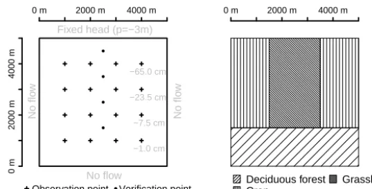
Figure 5. Synthetic set-up for the twin experiment. The left hand figure shows boundary conditions of the subsurface model (ParFlow) and the location of observation (crosses) and verification (filled circles) points. Grey numbers indicate the depth of observation and verification nodes, which are constant in west–east direction. The right hand figure shows the spatial distribution of plant functional types used in the land surface model (CLM).
is set up for the land surface–subsurface part of TerrSysMP (CLM+ParFlow). A synthetic reference run with prede-fined subsurface parameters (spatially distributed field of sat-urated hydraulic conductivityKs) provides virtual measure-ment data of soil moisture content for several observation locations. The ensemble for the data assimilation experi-ment consists of different realisations for spatially distributed saturated hydraulic conductivity and different precipitation rates. The synthetic soil moisture observation data are used to jointly update soil water content and saturated hydraulic conductivity with EnKF on a daily basis.
5.1 Experimental set-up
The domain of the virtual catchment has a horizontal exten-sion of 5000 m×5000 m and is discretised into 200×200 grid cells with a grid cell size of 25 m×25 m (see Fig. 5). The subsurface domain (modelled with ParFlow) has a verti-cal extension of 13 m, which is discretised into 20 cells with variable thickness. The uppermost 10 subsurface layers in ParFlow have an exponentially increasing profile with depth, corresponding to the soil layer thicknesses in CLM. These 10 layers sum up to a total thickness of 3 m. Note that for these 10 layers, pressure, saturation and land surface fluxes are ex-changed between CLM and ParFlow (see Sect. 2). The 10 re-maining subsurface layers have a constant thickness of 1 m. The topography of the model domain is flat, which means that there is no topographically driven overland flow within the domain. The porosity is set to a value of 0.4 m3m−3and the specific storage to 1×10⁻⁴m−1and both are spatially constant throughout the subsurface domain. Variably satu-rated flow was parameterised with the van Genuchten model (van Genuchten, 1980). The van Genuchten parameters α
andnwere both set to a spatially constant value of 2.0 m−1 and 2.0, respectively.
The land surface is covered by three vegetation types (i.e. plant functional types) in this example: deciduous forest,
cropland and grassland (see Fig. 5). The meteorological forc-ings (Fig. 6) are taken from reanalysis data of the German Weather Service (DWD) for the year 2013 for a grid cell close to Jülich (Germany) and the assigned meteorological forcings are spatially homogeneous within the virtual catch-ment. The boundary conditions for the subsurface domain are no flow in the southern, eastern and western faces and a con-stant head boundary condition (water table depth of−3 m) at the northern face. The initial groundwater table in all simula-tions is linearly decreasing from−2 m at the southern bound-ary to−3 m at the northern boundary.
For the data assimilation experiments a synthetic reference run was created with the model mentioned above. The syn-thetic reference field of log10(Ks)was generated with two di-mensional unconditioned sequential Gaussian simulation us-ing the gstat package (Pebesma, 2004) in the statistical soft-ware R (R Core Team, 2015). A spherical variogram with a nugget of 0.0 log10(m h−1), a sill of 0.1 log10(m2h−2)and a range of 70 model grid cells (1750 m) was used for the simulations. A constant value of−3 log10(m h−1)was added to the generated log10(Ks)field and the final field was as-signed to each model layer. The synthetic reference simula-tion was run for 6 months (January–June 2013, 181 days) with an hourly time step for both ParFlow and CLM. Obser-vation data (soil water content) from this reference run are collected at 16 observation points (Fig. 5), which are evenly distributed over the whole virtual catchment. Observations are taken at different depths ranging from the uppermost model layer (−1 cm) in the south to the sixth model layer (−65 cm) in the north. Additionally, four verification points are defined to assess the effect of soil moisture assimilation in between the observation points.
Figure 6. Hourly meteorological forcings for twin experiment from 1 January to 30 June 2013. Left panel shows 2 m air temperature and precipitation, middle panel shows incoming short-wave radiation and right panel shows incoming long-wave radiation.
for the reference field. Only the sill value was increased to 0.2 log10(m2h−2). The ensemble of meteorological forc-ings was generated by perturbing precipitation rates from the DWD reanalysis data with multiplicative noise sampled from a uniform distributionU (0.5,1.5). For each realisation, daily perturbation factors were sampled from the uniform distribu-tion and the hourly precipitadistribu-tion values were multiplied with the corresponding perturbation factor. The daily perturbation factors were randomly sampled; i.e. no temporal correlation was considered.
First, the ensemble was used to perform an open-loop simulation (i.e. no observation data are assimilated) for the whole simulation period (January–June 2013). This simula-tion serves as a spin-up and benchmark for the following data assimilation run. Data assimilation was performed for the second half of the simulation period (April–June 2013) after the ensemble was spun-up for the first 3 months (January– March). Observation data from the reference run (soil mois-ture content) were assimilated on a daily basis for all 16 observation points. The measurement error for all observa-tions was set to 0.02 m3m−3 and measurement errors were assumed to be spatially uncorrelated. The measurement data were used to jointly update the pressure and log10(Ks)fields in ParFlow with an augmented state vector approach, result-ing in 1.6 million unknowns for the data assimilation prob-lem.
5.2 Scaling behaviour of TerrSysMP–PDAF
In order to check the computational efficiency of TerrSysMP–PDAF in a high-performance computational environment, we performed a weak scaling study on the supercomputer JUQUEEN located at Forschungszentrum Jülich (Germany). JUQUEEN consists of 28 672 IBM Blue-Gene/Q compute nodes with a total of 458 752 processors and 448 TB main memory. Each compute node consists of 17 cores (16 for computation, 1 for operating system services) running at 1.6 GHz and 16 GB main memory. The compute nodes allow for simultaneous multi-threading (SMT) up to a factor of 4, which means that up to 64 processes can run on one node. JUQUEEN uses a static memory mapping
to processors, so one processor can utilise a maximum of 1 GB main memory (256 MB in case of four-way SMT). The whole system reaches a Linpack performance of 5.0 Petaflops. More details on the system architecture of JUQUEEN can be found in Gasper et al. (2014).
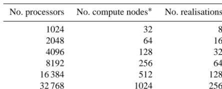
In a weak scaling study, which is typically performed for such kinds of systems, the workload per processor is held constant and the problem size linearly increases with the number of processors. As we are not interested in the scaling properties of TerrSysMP itself, which have been described in detail by Gasper et al. (2014), we keep the number of processors for each model realisation constant and increase the number of model realisations along with the number of processors. For the scaling study, the synthetic model set-up described in Sect. 5.1 is used but only the first 20 assimila-tion time steps (1–20 April 2013) are calculated. For each model realisation 128 processors were used, which keeps the workload per processor constant. The partitioning of proces-sors for one realisation was 96 for ParFlow and 32 for CLM, which was found to be the most optimal ratio for both mod-els in terms of simulation time and computational efficiency. Furthermore, preliminary tests suggested that using 32 pro-cessors per node (two-way SMT) on JUQUEEN was the best compromise between execution time and memory require-ments of ParFlow and CLM. For the weak scaling study, the number of realisations was increased from 8 to 256 and the corresponding number of processors ranged from 1024 to 32 768. Between each step of the scaling the number of re-alisations and processors was doubled (see Table 1 for infor-mation on all investigated scaling steps). The lowest number of realisations (processors) was set to 8 (1024) because this is the lowest possible job size on JUQUEEN given our cho-sen set-up (128 processors per model realisation, 32 ranks per compute node). The scaling behaviour can be assessed by calculating parallel efficiencyEfor weak scaling:
E(np)=
T1024
T (np)
, (1)
informa-Table 1. Number of processors, compute nodes and realisation used in the weak scaling study for TerrSysMP–PDAF on JUQUEEN. Each realisation was computed with a constant number of proces-sors for ParFlow (96) and CLM (32).
No. processors No. compute nodes∗ No. realisations
1024 32 8
2048 64 16
4096 128 32
8192 256 64
16 384 512 128
32 768 1024 256
∗A compute node on JUQUEEN consists of 16+1 physical cores but allows
for simultaneous multi-threading up to a factor of 4. For the weak scaling study 32 ranks per compute node were used for simulations.
tion for the weak scaling study was acquired by instrument-ing TerrSysMP–PDAF with the parallel performance tool Scalasca (Geimer et al., 2010) (version 2.2.1). Note that no special optimisation (such as critical path analysis) was per-formed to acquire the timing information with Scalasca.
A specific problem that occurs for assessing the paral-lel performance of ensemble methods like the EnKF in TerrSysMP–PDAF is that the simulation times for different ensemble members varies according to the assigned forcings and parameter sets. This, of course, can introduce some load balance issues because the filtering step introduces an effec-tive barrier for the parallel computation. This implicit barrier causes the processors, for which the computation of the spe-cific realisation is already finished for the current time step, to wait until the computation of the remaining model realisa-tions is finished before they can proceed to the filtering step. This is typically not the case when parallel performance is measured for a deterministic model (as for example in Kol-let et al., 2010; Gasper et al., 2014). In this case, the same model set-up is extended spatially for keeping a fixed work-load per processor, meaning that the internal model processes during the calculation stay the same when the weak scaling behaviour is assessed by simultaneously increasing the do-main size and the number of processors.
Therefore, the scalability of TerrSysMP–PDAF was first tested with a homogeneous ensemble where all ensemble members are identical to the reference run that was used to generate the observation data. This means that for all en-semble members the reference log10(Ks)field and the de-terministic (unperturbed) forcings were used. As a result, there is no variability in the ensemble for this set-up. Al-though this idealised set-up is not meaningful from a method-ological perspective (as all ensemble members are identical) this will provide information about the scaling of TerrSysMP in a pure technical sense and helps to gain insight into the computational limits for performing data assimilation with TerrSysMP in a massively parallel environment. In a second step, the scaling was investigated for the heterogeneous
en-semble that is described in Sect. 5.1. For this set-up, also the load imbalance caused by variable forcing and parameter sets is taken into account in the scaling results. Note that re-sults from this scaling set-up heavily depend on the chosen uncertainty description and the model dynamics of the cho-sen assimilation time period. Furthermore, the settings of the solver and the time stepping that is used to solve the transient variably saturated groundwater flow equations in ParFlow influence the scaling behaviour in this case. Therefore, re-sults from this study are only meant to provide an example on how the scaling could look like for a typical application of TerrSysMP–PDAF for a coupled land surface–subsurface environment. In this study, no attempt was made to optimise the time stepping and solver settings of ParFlow in order to decrease load imbalance issues.
Aside from the above-mentioned effect of ensemble het-erogeneities, another important issue that influences the par-allel performance of data assimilation algorithms are the in-put/output (I/O) settings of the model code. Compared to a deterministic model run, the I/O operations multiply with the number of realisations in a data assimilation run. This can create a certain bottle neck for the code performance when large amounts of output data are written to disk si-multaneously. Usually, in data assimilation applications the model output is restricted to the most important variables and mostly include the assimilated state variable and pos-sibly other state variables or parameters that are jointly up-dated with measurement data or provide diagnostic informa-tion on the model performance. In some cases, detailed in-formation on the distribution of certain variables is required, which means that output files from all ensemble members are needed for this variable. In other cases, knowledge on the statistics (e.g. mean and standard deviation) of a certain vari-able is sufficient. As ensemble output might be of importance for the parallel efficiency, we also compared three scenarios with a varying degree of model output:
– no model output;
– mean and standard deviation of simulated pressure and updated log10(Ks) fields are calculated during model execution and are written to file by the filter commu-nicator;
– output files for simulated pressure and updated log10(Ks)fields are written for all ensemble members. These three I/O scenarios were compared for the idealised test case (homogeneous ensemble) as well as the test case with a heterogeneous ensemble. This gives a total of six scal-ing scenarios. For each of these scenarios, the parallel effi-ciency was calculated with Eq. (1) separately meaning that the parallel efficiency is always normalised to the respective simulation with 1024 processors (T1024).
Figure 7. Scaling behaviour (left) and timing information (right) for TerrSysMP–PDAF for a weak scaling test on JUQUEEN. Black lines show results for an idealised test case (identical ensemble members) and grey lines show results for a heterogeneous ensemble. The number of ensemble members is increased from 8 to 256. Each ensemble member used 32 processors for CLM and 96 processors for ParFlow.
(heterogeneous ensemble) scaling runs. The parallel effi-ciency for the ideal test case stays very high (>0.8) for all output scenarios within the investigated range of resources. The scenarios with model output show a slight reduction of parallel efficiency for a higher number of processors (>
8192). From the absolute timing information one can see that the scenario with full ensemble output requires systemati-cally more time than the scenarios with no model output and statistical output only. The scenario with statistical output re-quires approximately the same simulation time as the no I/O scenario for a lower number of processors but then levels off for higher processor numbers (>8192).
The parallel efficiency with the more realistic setting (het-erogeneous ensemble) in Fig. 7 generally shows a stronger and faster decrease with increasing resource allocation. The differences to the ideal test case are of the order of 10– 20 %, which is mainly caused by the load imbalance within the heterogeneous ensemble. Nevertheless, the parallel effi-ciency for the heterogeneous set-up is still around 0.6 for the largest tested processor allocation. From the timing informa-tion in Fig. 7 one can see that the scenario with full ensem-ble output requires more CPU time than the other scenarios for a lower number of processors. For a higher resource al-location, the differences between the I/O scenarios tend to vanish, which is a significant difference to the idealised test case. This behaviour is probably related to the load imbal-ance within the ensemble, which leads to a certain time delay in the writing of output files. On the contrary, in the idealised test case all ensemble members finish the model forward in-tegration at approximately the same time meaning that all ensemble members tend to write output files synchronously. Note that for the heterogeneous case, an offline coupling be-tween TerrSysMP and PDAF would also lead to a certain time overhead due to I/O operations because the writing and reading of restart files after the assimilation step would also occur simultaneously before the next model integration.
More detailed information on the timing of individual components of TerrSysMP–PDAF for the idealised scenario
Figure 8. Timing information for individual components of TerrSysMP–PDAF for three I/O scenarios for the ideal test case.
end of the assimilation phase (updated Ks). In the finalisa-tion phase there is also a certain offset for the scenario with full ensemble output but the required computation time is in general very low compared to the other parts of the program. The scaling results for the idealised set-up are in gen-eral very good as the parallel efficiency stays above 0.8 even for a large number of processors. This is an indica-tion that the coupling between TerrSysMP and PDAF is working very well in a technical sense. Furthermore, the re-sults show that the filter algorithms implemented in PDAF scale well to an even higher number of processors than re-ported before in Nerger and Hiller (2013). The bottleneck of the parallel performance is mainly the initialisation phase (reading operations and set-up of OASIS-MCT communica-tion) and the output operations. Here, parallel I/O concepts could help to further improve the parallel performance of TerrSysMP–PDAF. The scaling results for the more realistic heterogeneous ensemble are also promising for the applica-tion of TerrSysMP–PDAF for more complex land surface– subsurface data assimilation problems. Generally, for any given model set-up, the scaling behaviour of the data as-similation problem will particularly depend on the numer-ical robustness of the deterministic forward model towards ensemble perturbations. Critical situations with respect to convergence could occur, e.g. for strong heterogeneities in the subsurface parameterisation (e.g. hydraulic conductivi-ties) or for the coupling of overland and subsurface flow. For the latter case, especially the computationally demanding on-set and offon-set of overland flow at particular grid cells (e.g. due to heavy rainfall or recession events) can have a negative influence on the scaling behaviour of the deterministic for-ward model (Kollet and Maxwell, 2006; Osei-Kuffuor et al.,
2014). If only a subset of realisations is affected by such convergence problems, also the scalability of the ensemble propagation might be influenced negatively. Therefore, it is important to configure the deterministic forward model well with respect to numerical stability and execution time. This can be achieved, for example, through the correct choice of solver parameters, an adequate spatio-temporal discretisation of the problem and a proper choice of model parameters and ensemble perturbations.
5.3 Data assimilation results
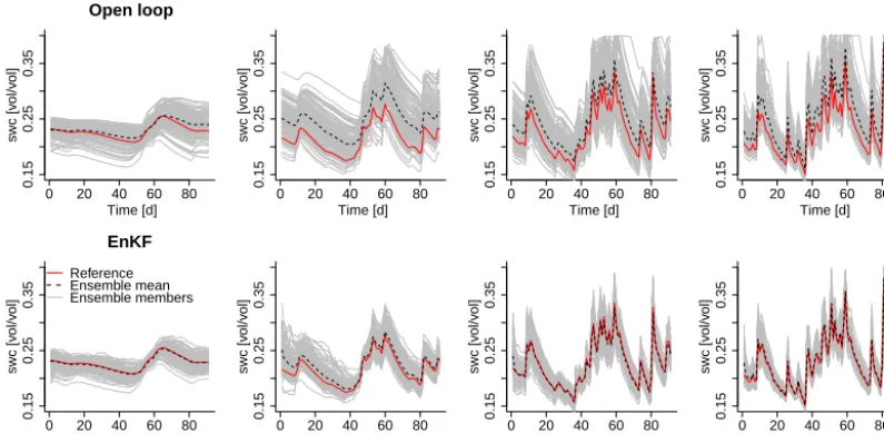
Figure 9 shows time series of simulated soil water content at four verification points (see Fig. 5) along the south–north direction for both the open loop (upper row) and the assimi-lation run (lower row). Results for the open-loop simuassimi-lations already show that the temporal dynamics of the reference run are well represented by the ensemble and that the changes in soil moisture very much depend on the dynamics of the me-teorological forcing data. Assimilation of soil moisture data leads to a reduction of the ensemble spread and a reduction of the mismatch between the ensemble mean of forecasted soil moisture and the reference values. Additionally the ab-solute average error (AAE) of soil moisture contentθis used to assess the model performance of the open loop and the assimilation run:
AAEθ =
1
Nt Nt X
i
| ¯θisim−θiref|, (2)
whereθ¯sim is the ensemble mean of simulated soil mois-ture, θref is the reference soil moisture content and Nt is
0 20 40 60 80
0.15
0.25
0.35
Open loop
Time [d]
swc [v
ol/v
ol]
0 20 40 60 80
0.15
0.25
0.35
EnKF
Time [d]
swc [v
ol/v
ol]
Reference Ensemble mean Ensemble members
0 20 40 60 80
0.15
0.25
0.35
Time [d]
swc [v
ol/v
ol]
0 20 40 60 80
0.15
0.25
0.35
Time [d]
swc [v
ol/v
ol]
0 20 40 60 80
0.15
0.25
0.35
Time [d]
swc [v
ol/v
ol]
0 20 40 60 80
0.15
0.25
0.35
Time [d]
swc [v
ol/v
ol]
0 20 40 60 80
0.15
0.25
0.35
Time [d]
swc [v
ol/v
ol]
0 20 40 60 80
0.15
0.25
0.35
Time [d]
swc [v
ol/v
ol]
Figure 9. Simulated soil water content at the four verification nodes in Fig. 5 (from north to south) for April–June 2013 (91 days). Upper row shows results for open-loop simulations and lower row for assimilation.
the uppermost 10 model layers reduced from 0.0135 m3m−3 (open-loop simulation) to 0.0096 m3m−3 (assimilation ex-periment) through the assimilation of soil moisture data (the 10 lower model layers were excluded from this calculation because they are constantly saturated during the whole sim-ulation period). In Fig. 10 AAEθ is shown for one specific
model layer at −65 cm depth. It can be seen from Fig. 10 that AAEθ is reduced in large parts of the model domain,
which means that data assimilation was not only effective at the observation locations but also significantly improved the model performance in the surrounding grid cells. Sev-eral spots in the model domain, e.g. at the southern bound-ary and in the north-east, show less improvement, which may be related to the assigned boundary conditions and the fact that the distance to observation points is larger at the model boundaries reducing the correlation between obser-vation points and those grid cells. The effect of soil mois-ture assimilation on land surface fluxes (latent and sensible heat flux) was also analysed for this set-up. The total AAE values (averaged over all grid cells and time steps) in the open-loop run were 1.003 W m−2for sensible heat flux and 1.212 W m−2for latent heat flux. The spatial pattern of errors in land surface fluxes is closely related to those of AAEθ in
Fig. 10. In principal, the calculation of land surface fluxes within TerrSysMP can be affected by (1) plant physiological parameters, (2) meteorological forcings that affect stomatal conductance and (3) the availability of water in the subsur-face. In the chosen set-up neither plant physiological param-eters nor meteorological forcings (with the exception of pre-cipitation) were perturbed, so the variability of land surface fluxes is mainly influenced by the availability of water in the rooting zone. The relatively low errors in the open-loop sim-ulation indicate that the variability of soil moisture content
only had a limited effect on land surface fluxes in the cho-sen set-up and that most of the model domain is not affected by water limitation. With the assimilation of soil moisture contents, the total AAE values of sensible (latent) heat fluxes were reduced to 0.730 (0.876) W m−2, which is a relative im-provement of about 27 %. Nevertheless, the absolute magni-tude of land surface flux errors and the improvements by data assimilation are relatively low due to the fact that the system was not affected by water limitation throughout the simula-tion period.
In the presented data assimilation experiment, soil mois-ture data from the reference run are also used to simultane-ously update the log10(Ks)fields of the ensemble. In Fig. 11 the reference field of log10(Ks)is compared with the aver-age log10(Ks)field of the initial ensemble and the average log10(Ks)field after the assimilation period. It becomes ob-vious that the correction of log10(Ks)values through the as-similation of soil moisture observations leads to a significant improvement of the estimated average log10(Ks)field. Com-pared to the initial estimate of log10(Ks), the updated average log10(Ks)field includes the main structural features of the reference field, e.g. the higher log10(Ks)values in the east-ern part and the lower values in the westeast-ern part. Again, as for AAEθ, the improvement is less pronounced at the model
boundaries especially in the southern part. This can again be related to the lower observation density at the model borders. 5.4 Applicability at hyper-resolution
con-Figure 10. Absolute average error of soil water content AAEθfor open loop (left) and assimilation (right) at a depth of−65 cm from April
to June 2013.
Figure 11. Log-transformed saturated hydraulic conductivity fields of the reference (left), the initial ensemble mean (middle) and the updated ensemble mean at the end of the assimilation period (right).
tinuously moving forward towards higher model resolutions (e.g. Maxwell et al., 2015), which was identified as one of the forthcoming challenges in Earth system modelling (e.g. Wood et al., 2011; Bierkens et al., 2014). Therefore, it was also tested whether the TerrSysMP–PDAF data assimilation framework is applicable for models with a much bigger prob-lem size.
For this purpose, the problem size of the forward model was increased by a factor of 25 by increasing the horizontal model resolution to 5 m (1000×1000 grid cells) leading to 20 million grid cells for the subsurface part of TerrSysMP.
The model input for the synthetic reference and the en-semble was re-gridded to this higher model resolution. The log10(Ks)fields for the synthetic reference and the individual ensemble members were additionally perturbed with small-scale noise, which was introduced to resemble a certain sub-scale variability within the original 25 m grid cells. The small-scale perturbation fields were generated with the par-allel Gaussian simulation algorithm implemented in ParFlow with a horizontal correlation length of 20 m and a standard deviation of 0.2 log units. The reference log10(Ks)fields for
the 25 and 5 m resolution models are shown in Figs. 11 and 12, respectively. The set-up for the data assimilation experi-ment for the high-resolution model was identical to the 25 m resolution case, i.e. 90 days of model spin-up and daily as-similation of 16 soil moisture observations for 91 days with a joint state–parameter estimation.
Figure 12. Log-transformed saturated hydraulic conductivity fields of the reference (left), the initial ensemble mean (middle) and the updated ensemble mean at the end of the assimilation period (right) for the 5 m resolution model.
Of course, the model set-up that was used here is rel-atively simple in terms of model dynamics compared to typical real-world applications of integrated Earth system models. Topography, heterogeneous land surface parame-ters and spatially distributed meteorological forcings usually lead to a much more complex model behaviour, which also leads to far longer simulation times compared to the model set-up used in this study. This will make data assimilation with high-resolution integrated models for real-world appli-cations very challenging with respect to the amount of nec-essary computational resources. Nevertheless, these simula-tions with a relatively simple high-resolution model set-up show that the TerrSysMP–PDAF framework is technically able to cope with data assimilation problems where the prob-lem size of the forward model is in the range of tens of millions grid cells. Such problem sizes will become more common especially in the context of integrated hydrologi-cal modelling on the catchment shydrologi-cale (e.g. to better resolve small-scale variabilities in hydraulic parameters) as well as for large-scale applications in order to improve hydrological and meteorological forecasts on the basin and the continental scale.
6 Conclusions and outlook
In this paper, we presented a modular high-performance data assimilation framework for the land surface–subsurface part of the integrated terrestrial system modelling platform TerrSysMP. In TerrSysMP, land surface processes are mod-elled with CLM 3.5 and subsurface processes with ParFlow where both models are coupled via the exchange of states and fluxes with the coupling software OASIS-MCT. The data assimilation system for this model was established with the Parallel Data Assimilation Framework (PDAF), which pro-vides a suite of efficient and scalable data assimilation algo-rithms. The coupling between TerrSysMP and PDAF is done in a fully integrated fashion meaning that the model ensem-ble as well as the infrastructure for data assimilation is only
initialised once and the data assimilation system is continu-ously integrated forward in time without the need of system calls to the model or re-initialisation of any of the system components. The data exchange between TerrSysMP and PDAF is done completely via main memory, which avoids the need for a frequent reading and writing of model restart files. TerrSysMP as well as PDAF are fully parallelised and the data exchange between the two components makes ef-fective use of the domain decomposition in the models. This significantly reduces the memory requirements of the system because the global state(-parameter) vector does not need to be stored completely in any part of the filter algorithm. In addition to the parallelism in the model integration (provided by the component models of TerrSysMP) and in the filter-ing step (provided by PDAF) also the ensemble propagation is running fully parallel. The data assimilation system for TerrSysMP is designed in a modular fashion; i.e. assimila-tion can either run with the coupled land surface–subsurface model (ParFlow+CLM coupled via OASIS-MCT) or with one of the stand alone models (ParFlow or CLM). This pro-vides the user with some flexibility regarding the model choice because for certain modelling purposes the use of a single compartment model (subsurface or land surface) may be sufficient in the context of data assimilation, whereas in other situations a fully coupled approach may be more adequate. Currently, pressure and soil moisture data can be assimilated in ParFlow. These data are used in ParFlow for a state update of the 3-D pressure field but they can also be used for a joint update of saturated hydraulic conductivities or Mannings coefficients. If the assimilation system is only running with CLM, soil moisture data can be assimilated di-rectly into CLM.
high-resolution models, which require a huge amount of compu-tational resources and therefore also benefit from an efficient implementation of the ensemble propagation and the filter-ing step. Additional tests with a high-resolution model set-up where 20 million states and 20 million parameters were up-dated simultaneously (as compared to 0.8 million states and 0.8 million parameters in the scaling study) revealed that the infrastructure of the proposed TerrSysMP–PDAF framework is well suited for such large problem sizes. Results from the scaling study also showed that the output strategy (ensemble output vs. statistical output) as well as load balancing issues between the different ensemble members can have a certain influence on the parallel efficiency, which should be carefully taken into consideration when data assimilation is performed with a large amount of computational resources.
In further work we plan to include also the atmospheric compartment model of TerrSysMP (COSMO-DE) in the as-similation system. This will allow us to investigate the effect of data assimilation in a fully coupled system from the sub-surface to the atmosphere. It is also planned to extend the data assimilation system to make full use of the functionality of PDAF with respect to filter variants and assimilation op-tions (e.g. localisation and smoothing). Furthermore, the data assimilation system will be extended with additional mea-surement operators for soil moisture assimilation including measurement operators for active and passive radar remote sensing data and cosmic ray sensors.
Code availability
The source code of TerrSysMP–PDAF is added as a supple-ment to this article.
The Supplement related to this article is available online at doi:10.5194/gmd-9-1341-2016-supplement.
Author contributions. Guowei He and Wolfgang Kurtz developed
the model code. Harrie-Jan Hendricks Franssen, Stefan J. Kollet and Wolfgang Kurtz designed the simulation experiments and Wolf-gang Kurtz carried them out. Reed M. Maxwell and Stefan J. Kollet provided consultancy for the ParFlow and TerrSysMP model code. Wolfgang Kurtz prepared the manuscript with contributions from all co-authors. Harrie-Jan Hendricks Franssen, Stefan J. Kollet and Harry Vereecken provided guidance for the work and acquired the necessary project funding.
Acknowledgements. The authors gratefully acknowledge the
computing time granted by the JARA-HPC Vergabegremium and provided on the JARA-HPC partition part of the supercomputer JUQUEEN at Forschungszentrum Jülich. This work was supported by SFB-TR32 “Patterns in soil–vegetation–atmosphere systems:
monitoring, modelling and data assimilation” funded by the German Science Foundation (DFG). Further support was provided by the Helmholtz Alliance on “Remote Sensing and Earth System Dynamics”. The authors also wish to thank three anonymous reviewers for their constructive comments and suggestions, which greatly improved the quality of the manuscript.
The article processing charges for this open-access publication were covered by a Research
Centre of the Helmholtz Association.
Edited by: M.-H. Lo
References
Anderson, J. L.: An ensemble adjustment Kalman filter for data assimilation, Mon. Weather Rev., 129, 2884–2903, doi:10.1175/1520-0493(2001)129<2884:AEAKFF>2.0.CO;2, 2001.
Anderson, J., Hoar, T., Raeder, K., Liu, H., Collins, N., Torn, R., and Avellano, A.: The data assimilation research testbed: a community facility, B. Am. Meteorol. Soc., 90, 1283–1296, doi:10.1175/2009bams2618.1, 2009.
Andreadis, K. M. and Lettenmaier, D. P.: Assimilating re-motely sensed snow observations into a macroscale hydrology model, Adv. Water Resour., 29, 872–886, doi:10.1016/j.advwatres.2005.08.004, 2006.
Ashby, S. and Falgout, R.: A parallel multigrid preconditioned conjugate gradient algorithm for groundwater flow simulations, Nucl. Sci. Eng., 124, 145–159, 1996.
Bailey, R. T. and Baù, D.: Estimating geostatistical parameters and spatially-variable hydraulic conductivity within a catchment sys-tem using an ensemble smoother, Hydrol. Earth Syst. Sci., 16, 287–304, doi:10.5194/hess-16-287-2012, 2012.
Baldauf, M., Seifert, A., Förstner, J., Majewski, D., Raschendor-fer, M., and Reinhardt, T.: Operational convective-scale nu-merical weather prediction with the COSMO model: descrip-tion and sensitivities, Mon. Weather Rev., 139, 3887–3905, doi:10.1175/mwr-d-10-05013.1, 2011.
Barbu, A. L., Calvet, J.-C., Mahfouf, J.-F., and Lafont, S.: Integrat-ing ASCAT surface soil moisture and GEOV1 leaf area index into the SURFEX modelling platform: a land data assimilation application over France, Hydrol. Earth Syst. Sci., 18, 173–192, doi:10.5194/hess-18-173-2014, 2014.
Barker, D., Huang, X.-Y., Liu, Z., Auligné, T., Zhang, X., Rugg, S., Ajjaji, R., Bourgeois, A., Bray, J., Chen, Y., Demirtas, M., Guo, Y.-R., Henderson, T., Huang, W., Lin, H.-C., Michalakes, J., Rizvi, S., and Zhang, X.: The Weather Research and Fore-casting Model’s Community Variational/Ensemble Data Assim-ilation System: WRFDA, B. Am. Meteorol. Soc., 93, 831–843, doi:10.1175/bams-d-11-00167.1, 2012.
Bateni, S. and Entekhabi, D.: Surface heat flux estimation with the ensemble Kalman smoother: joint estimation of state and parameters, Water Resour. Res., 48, W08521, doi:10.1029/2011WR011542, 2012.