CHIMERE 2013: a model for regional atmospheric composition modelling

(1)

Geosci. Model Dev., 6, 981–1028, 2013 www.geosci-model-dev.net/6/981/2013/ doi:10.5194/gmd-6-981-2013

EGU Journal Logos (RGB)

Advances in

Geosciences

Open Access

Natural Hazards

and Earth System

Sciences

Open Access

Annales

Geophysicae

Open Access

Nonlinear Processes

in Geophysics

Open Access

Atmospheric

Chemistry

and Physics

Open Access

Atmospheric

Chemistry

and Physics

Open Access

Discussions

Atmospheric

Measurement

Techniques

Open Access

Atmospheric

Measurement

Techniques

Open Access

Discussions

Biogeosciences

Open Access Open Access

Biogeosciences

Discussions

Climate

of the Past

Climate

of the Past

Discussions

Earth System

Dynamics

Earth System

Dynamics

Discussions

Geoscientific

Instrumentation

Methods and

Data Systems

Open Access

_{Geoscientific}

Instrumentation

Methods and

Data Systems

Open Access

Discussions

Geoscientific

Model Development

Geoscientific

Model Development

Discussions

Hydrology and

Earth System

Sciences

Open Access

Hydrology and

Earth System

Sciences

Open Access

Discussions

Ocean Science

Discussions

Solid Earth

Discussions

The Cryosphere

Discussions

Natural Hazards

and Earth System

Sciences

Open Access

Discussions

CHIMERE 2013: a model for regional atmospheric

composition modelling

L. Menut1, B. Bessagnet2, D. Khvorostyanov1, M. Beekmann3, N. Blond4, A. Colette2, I. Coll3, G. Curci5, G. Foret3, A. Hodzic6, S. Mailler1, F. Meleux2, J.-L. Monge1, I. Pison7, G. Siour3, S. Turquety1, M. Valari1, R. Vautard7, and M. G. Vivanco8

1_{Laboratoire de M´et´eorologie Dynamique, IPSL, CNRS, UMR8539, 91128 Palaiseau Cedex, France}

2_{Institut national de l’environnement industriel et des risques, Parc technologique ALATA, 60550 Verneuil en Halatte, France} 3_{Laboratoire Interuniversitaire des Systèmes Atmosphériques, IPSL, CNRS, UMR 7583, Université Paris Est Créteil (UPEC)}

and Universit´e Paris Diderot (UPD), Cr´eteil, France

4_{Laboratoire Image Ville Environnement, CNRS/UDS, UMR7362, Strasbourg, France}

5_{Dipartimento di Scienze Fisiche e Chimiche – CETEMPS, Universita degli Studi dell’Aquila, L’Aquila, Italy} 6_{NCAR Atmospheric Chemistry Division, 3450 Mitchell Lane, Boulder, Colorado, USA}

7_{Laboratoire des Sciences du Climat et de l’Environnement, IPSL, CEA-CNRS-UVSQ, UMR8212, Gif sur Yvette, France} 8_{Environment Department, CIEMAT, Madrid, Spain}

Correspondence to: L. Menut ([email protected])

Received: 23 November 2012 – Published in Geosci. Model Dev. Discuss.: 21 January 2013 Revised: 11 June 2013 – Accepted: 12 June 2013 – Published: 22 July 2013

Abstract. Tropospheric trace gas and aerosol pollutants have adverse effects on health, environment and climate. In order to quantify and mitigate such effects, a wide range of pro-cesses leading to the formation and transport of pollutants must be considered, understood and represented in numer-ical models. Regional scale pollution episodes result from the combination of several factors: high emissions (from anthropogenic or natural sources), stagnant meteorological conditions, kinetics and efficiency of the chemistry and the deposition. All these processes are highly variable in time and space, and their relative contribution to the pollutants budgets can be quantified with chemistry-transport models. The CHIMERE chemistry-transport model is dedicated to regional atmospheric pollution event studies. Since it has now reached a certain level a maturity, the new stable ver-sion, CHIMERE 2013, is described to provide a reference model paper. The successive developments of the model are reviewed on the basis of published investigations that are ref-erenced in order to discuss the scientific choices and to pro-vide an overview of the main results.

1 Introduction

The rapid growth of urban areas and increased industriali-sation have created the need for air quality assessment and motivated the first regional-scale studies on anthropogenic pollution in the early 1990s (Fenger, 2009, among others). The first systematic measurements have been implemented by the air quality agencies in the source regions, which often coincided with the most densely populated areas. One of the first targeted pollutants was sulphur dioxide due to its effects on acid rain and forest ecosystems.

(2)

982 L. Menut et al.: CHIMERE: a model for regional atmospheric composition modelling

Even if air pollution was considered as a local and mostly urban problem, it has been shown that ozone and its precur-sors may be transported over long distances. Therefore, to study local pollution and represent effects of anthropogenic and biogenic emissions, chemistry and transport on the lo-cal pollution budget, models need to integrate processes over large spatial scales. While early models were based on statis-tical assumptions and could not account for sporadic changes in the atmospheric forcing, the past two decades have seen the development of deterministic and Eulerian models. Some of these models are very complex and dedicated to field or idealised studies of a few days, over specific regions. Others are dedicated to long-range transport only. In addition, some models allow fast simulations and are thus suitable for daily forecast, Monks (2009).

The CHIMERE model has been in development for more than fifteen years and is intended to be a modular framework available for community use. It includes the necessary state-of-the-art parameterisations to simulate reasonable pollutant concentrations, but remains also computationally efficient for forecast applications. CHIMERE is also frequently used for field experiment analysis studies, long-range transport and trend quantification over continental scales. Designed for both the research community and operational agencies, the CHIMERE model needs to be computationally stable and provide robust results. This means that the model needs to be able to estimate pollution peaks at the right time and loca-tion, but also to be able to diagnose low pollution conditions and avoid false alerts. As a research tool, the model needs to be modular enough to allow adding new processes or testing specific physico–chemical interactions. In the present paper we describe the parameterisations included in the CHIMERE model and the results of recent studies explaining the ratio-nale of the last model improvements.

This paper represents the reference model description for CHIMERE version 2013. An overview of the CHIMERE model structure is given in Sect. 2. The domains defini-tion and the boundary condidefini-tions are described in Sect. 3. The meteorological forcings and their preprocessing are pre-sented in Sect. 4 and the implementation of transport and mixing is discussed in Sect. 5. The emissions taken into ac-count in the model (anthropogenic, biogenic, mineral dust, fires and the local resuspension of particulate matter) are de-scribed in Sect. 6. The gaseous and aerosol chemistries are presented in Sect. 7. The dry and wet deposition processes are presented in Sect. 8 and the cloud impacts in Sect. 9. The CHIMERE model results evaluations are discussed in Sect. 10. The hybridation between model and observations (for sensitivity, inverse modelling and data assimilation) are presented in Sect. 11. The experimental and operational fore-casts operated with CHIMERE are described in Sect. 12. Fi-nally, a summary and new research directions are presented in Sect. 14.

The main goal of this paper is to describe in detail all the numerical and scientific choices and to explain the main

reasons for these choices. In addition, ongoing and planned developments and application studies are presented.

2 CHIMERE model overview

2.1 Main characteristics

CHIMERE is an Eulerian off-line chemistry-transport model (CTM). External forcings are required to run a simula-tion: meteorological fields, primary pollutant emissions, and chemical boundary conditions. Using these input data, CHIMERE calculates and provides the atmospheric concen-trations of tens of gas-phase and aerosol species over local to continental domains (from 1 km to 1 degree resolution). The key processes affecting the chemical concentrations repre-sented in CHIMERE are emissions, transport (advection and mixing), chemistry and deposition, as presented in Fig. 1. Note that forcings have to be on the same grid and time step as the CTM simulation. In this sense, CHIMERE is not only a chemical model but a suite of numerous preprocess-ing programs able to prepare the simulation. The model is now used for pollution event analysis, scenario studies, op-erational forecast and more recently for impact studies of pollution on health (Valari and Menut, 2010) and vegetation (Anav et al., 2011).

The first model version was released in 1997 and was a box model covering the Paris area and included only gas-phase chemistry (Honoré and Vautard, 2000; Vautard et al., 2001). In 1998, the model was implemented for its first forecast ver-sion (Pollux) during the ESQUIF (Etude et Simulation de la QUalité de l’air en Ile de France) experiment (Menut et al., 2000b), again over the Paris area (Vautard et al., 2000). At the same time, the adjoint model was developed to estimate the sensitivity of concentrations to all parameters (Menut et al., 2000a). In 2001, the geographical domain was extended over Europe with a cartesian mesh (Schmidt et al., 2001) and the new experimental forecast platform (PIONEER) was set up. In 2003, the experimental forecast became operational with the PREV’AIR (French air quality forecasting and mapping system) system operated at INERIS (National Institute for In-dustrial Environment and Risks) (Honoré et al., 2008; Rou¨ıl et al., 2009). The aerosol module was implemented in 2004 (Bessagnet et al., 2004) with further improvements concern-ing the dust natural emissions and resuspension over Europe (Vautard et al., 2005, Hodzic et al., 2006a; Bessagnet et al., 2008) and evaluated against long-term and field measure-ments (Hodzic et al., 2005, 2006b). The development of the mineral dust version started in 2005 (Menut et al., 2005b). Chemistry was not included in that version and a new hori-zontal domain had to be designed to cover the whole north-ern Atlantic and Europe, including the Sahara and down-wind regions. In 2006, an important step was achieved with the development of the parallel version of the model and its first implementation on a massively parallel computer

(3)

L. Menut et al.: CHIMERE: a model for regional atmospheric composition modelling 983

Menut L.et al.: CHIMERE: a model for regional atmospheric composition modelling 3

Fig. 1. General principle of a chemistry-transport model such as CHIMERE. In the box ’Meteorology’,u∗stands for the friction velocity,

Q0the surface sensible heat flux,Lthe Monin-Obukhov length and BLH the boundary layer height. cmodandcobsare for the chemical

concentrations fields for the model and the observations, respectively.

on a web sitewww.lmd.polytechnique.fr/chimere. The docu-mentation is both technical and scientific. It includes a chap-ter dedicated to the set-up of a test case simulation that allows

175

new users to easily carry out a CHIMERE simulation: model configuration and data (meteorology and emissions files) are provided to simulate the 2003 heat wave in western Europe.

CHIMERE is a National Tool of the French Insti-tut des Sciences de l’Univers, meaning that support has

180

to be provided to the users of model. Two mailing lists exist for this support: [email protected] to send questions to the model developers and [email protected] to initiate discussions, ex-change programs or data between users. In addition,

two-185

day training courses are organised twice a year. Each training course is free of charge for participants and offers a complete training to be able to install the code, launch a simulation and change surface emissions or other parameters in the code.

The code is completely written in Fortran90, and running

190

scripts are written in shell (using gnu-awk for input datafiles processing). The required software is a Fortran 95 compiler (g95 and gfortran are both free and efficient, but Makefiles with Intel’s ifort compiler options are also provided). The re-quired libraries are NetCDF (either 3.6.x or 4.x.x), MPI (see

195

below), and GRIB API (associated to the use of the ECMWF meteorological datasets). The model includes tools that can help the user to configure the model’s Makefiles for the li-braries already installed.

The model computation time for one AMDx64 node of

200

16 CPUs is 1h30min for 1 month of simulation for the Paris

area, at 15 km resolution, the domain size being 45x48x8 with a time step of 360 seconds on average. CHIMERE uses the distributed memory scheme, and MPI message passing library. It is maintened for Open MPI (recommended) and

205

LAM/MPI, but works, with minor changes in the scripts, with MPICH or other MPI compatible parallel environ-ments. The model parallelism results from a Cartesian di-vision of the main geographical domain into several sub-domains, each one being processed by a worker process.

210

Each worker performs the model integration in its geographi-cal sub-domain as well as boundary condition exhanges with its neighbours. In addition a master process performs initial-isations and file input/output. To configure the parallel sub-domains, the user has to specify two parameters in the model

215

parameter file: the number of sub-domains for the zonal and meridional directions. The total number of CPUs used is therefore the product of these two numbers, plus one CPU for the master process.

For graphical postprocessing, simple interfaces are

avail-220

able using either the GMT 5 or the GrADS 6 free software. Also an additional graphical user interface (GUI) software CHIMPLOT is provided. It allows making various 1D or 2D plots (e.g., longitude-latitude or time-altitude maps, vertical slices, time series, vertical profiles). One can also overlay

225

multiple fields (e.g., O3 concentrations, wind vectors, and

pressure contours) and perform simple operations such as calculating daily maxima, daily means, vertical or horizon-tal averaging or integrations.

Fig. 1. General principle of a chemistry-transport model such as CHIMERE. In the box “Meteorology”,u∗stands for the friction velocity,

Q0the surface sensible heat flux,Lthe Monin–Obukhov length and BLH the boundary layer height.cmodandcobsare the modelled and the observed chemical concentrations fields, respectively.

(the ECMWF (European Centre for Medium-Range Weather Forecasts) computer within the framework of the FP6/GEMS (Global and regional Earth-system Monitoring using Satellite and in situ data) project).

The CHIMERE model is now considered a state-of-the-art model. It has been involved in numerous inter-comparison studies focusing mainly on ozone and PM10 from the urban

scale (Vautard et al., 2007; Van Loon et al., 2007; Schaap et al., 2007) to continental scale (Solazzo et al., 2012b; Zyryanov et al., 2012). The model has been mainly applied over Europe, and more recently over Africa and the North Atlantic for dust simulations, over Central America dur-ing the MILAGRO (Megacity Initiative: Local and Global Research Observations) project to study organic aerosols (Hodzic et al., 2009, 2010a,b), and over the US within the AQMEII (Air Quality Model Evaluation International Initia-tive) project (Solazzo et al., 2012b).

Finally, the development of CHIMERE follows three main rules. First, concentrations of main pollutants are calculated with the best possible accuracy using well evaluated and state-of-the-art parameterisations. Second, a modular frame-work is maintained to allow updates to the code by devel-opers and also all interested users. Third, the code is kept computationally efficient to allow long-term simulations, cli-matological studies and operational forecast.

2.2 The CHIMERE software

In order to facilitate software distribution, CHIMERE is pro-tected under the General Public License. This paper presents the latest model version release called CHIMERE 2013. The source code and the associated documentation is available on the website www.lmd.polytechnique.fr/chimere. The docu-mentation is both technical and scientific. It includes a chap-ter dedicated to the set-up of a test case simulation that allows new users to easily carry out a CHIMERE simulation: model configuration and data (meteorology and emissions files) are provided to simulate the 2003 heatwave in western Europe.

CHIMERE is a National Tool of the French Institut National des Sciences de l’Univers, meaning that support has to be provided to the users of model. Two mailing lists exist for this support: [email protected] to send questions to the model developers and [email protected] to initiate discussions, ex-change programs or data between users. In addition, two-day training courses are organised twice a year. Each training course is free of charge for participants and offers complete training to be able to install the code, launch a simulation and change surface emissions or other parameters in the code.

(4)

below), and GRIB API (associated to the use of the ECMWF meteorological datasets). The model includes tools that can help the user to configure the model’s Makefiles for the li-braries already installed.

The model computation time for one AMDx64 node of 16 CPUs is 1 h 30 min for 1 month of simulation for the Paris area, at 15 km resolution, the domain size being 45×48×8 with a time step of 360 s on average. CHIMERE uses the distributed memory scheme, and MPI message passing li-brary. It is maintained for Open MPI (recommended) and LAM/MPI, but works, with minor changes in the scripts, with MPICH or other MPI compatible parallel environ-ments. The model parallelism results from a Cartesian di-vision of the main geographical domain into several sub-domains, each one being processed by a worker process. Each worker performs the model integration in its geograph-ical sub-domain as well as boundary condition exchanges with its neighbours. In addition a master process performs initialisations and file input/output. To configure the paral-lel sub-domains, the user has to specify two parameters in the model parameter file: the number of sub-domains for the zonal and meridional directions. The total number of CPUs used is therefore the product of these two numbers, plus one CPU for the master process.

For graphical postprocessing, simple interfaces are avail-able using either the GMT 5 or the GrADS 6 free software. Also, an additional graphical user interface (GUI) software CHIMPLOT is provided. It allows making various 1-D or 2-D plots (e.g. longitude, latitude or time, altitude maps; ver-tical slices; time series; verver-tical profiles). One can also over-lay multiple fields (e.g. O3concentrations, wind vectors, and

pressure contours) and perform simple operations such as calculating daily maxima, daily means, vertical or horizon-tal averaging or integrations.

2.3 The CHIMERE code organisation

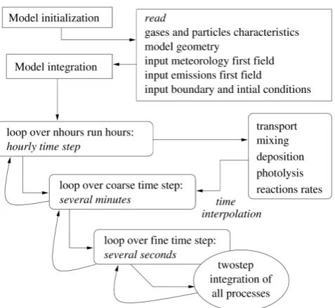
Apart from the preprocessing, i.e. the preparation of the forc-ing, the CHIMERE model is split into two main parts: an initialisation phase and the model integration phase (Fig. 2). The initialisation phase consists in reading all input param-eters as well as the preparation of the initial meteorological and chemical field.

The model integration phase is split into three stages: – An hourly time step that corresponds to the provision of

forcings, i.e. meteorological fields, emission fluxes and chemical boundary conditions.

– A user’s defined coarse time step “nphour”, correspond-ing to the time interpolation of “physical” parameters, such as wind, temperature, reactions rates, etc. In paral-lel, to optimise the time simulation and prevent issues associated to the violation of the Courant–Friedrich– Levy (CFL) criteria, a “physical” time step is dynam-ically estimated in the meteorological preprocessor,

4 Menut L.et al.: CHIMERE: a model for regional atmospheric composition modelling

2.3 The CHIMERE code organisation

230

Fig. 2.General CHIMERE structure for time integration of all pro-cesses

Apart from the pre-processing, i.e., the preparation of the forcing, the CHIMERE model is split into two main parts: an initialisation phase and the model integration phase ( Figure 2 ).

The initialisation phase consists in reading all input

param-235

eters as well as the preparation of the initial meteorological and chemical field.

The model integration phase is split into three stages:

– A hourly time-step that corresponds to the provision of forcings,i.e meteorological fields, emission fluxes and

240

chemical boundary conditions.

– A user’s defined coarse time step ’nphour’, correspond-ing to the time interpolation of ”physical” parameters, such as wind, temperature, reactions rates etc. In paral-lel, to optimise the time simulation and prevent issues

245

associated to the violation of the Courant-Friedrich-Levy (CFL) criteria, a ”physical” time step is dynami-cally estimated in the meteorological pre-processor tak-ing into account horizontal and vertical winds and deep convective updraft, as presented in Figure 3 . During

250

the run, if the specified time step is longer than the rec-ommended time step, the recrec-ommended time step will be used in model integrations. If the user’s defined time-step is shorter as the recommended one, the user’s choice is applied (even if this is not the optimal choice).

255

– A user’s defined fine time step ’ichemstep’: this corre-sponds to the integration of the chemical mechanism,

including concentration’s increments due to all pro-cesses. This is achieved by the two-step scheme. Due to the stiffness of the chemical system to solve, this time

260

step must be at least 30s (or less if possible). In prac-tice, for large domains, such as Western Europe, a ”very quick formulation” with a 10-minute physical step and no sub-chemical steps, i.e. all processes are stepped to 10 minutes, is realistic. It is possible to select one or two

265

Gauss-Seidel iterations, but the use of two iterations is strongly recommended even if it increases the computer time by two.

Fig. 3. Calculation of the number of integration steps per hour to respect the Courant-Friedrich-Levy (CFL) number over a complete 120 hours simulation. The CFL is estimated using three parame-ters: the mean wind speed|U|, the vertical wind speed in the envi-ronmentwand the vertical velocity in the updraft in case of active deep convection.

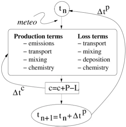
The numerical integration of all processes follows a production-loss budget approach as presented in Figure 4 .

270

This means that all production and loss terms, for each chemical species are calculated simultaneously to avoid error propagation generally created with operator-splitting tech-niques (the concentration evolution being dependent on the several terms order, McRae et al. (1982)). Further

advan-275

tages of the scheme are 1) its stability even for quite long time steps due to the implicitness of the formulation and 2) the simplicity of the code which facilitates the development of secondary models (adjoint, tangent linear).

The numerical method used to estimate the temporal

so-280

lution of the stiff system of partial differential equations is adapted from the second-order TWOSTEP algorithm orig-inally proposed by Verwer (1994)for gas phase chemistry only. It is based on the application of a Gauss-Seidel iter-ation scheme to the 2-step implicit backward differentiiter-ation

285

(BDF2) formula:

cn+1=4 3c

n₋1

3c

n−1₊2 3∆tR(c

n+1₎ ₍₁₎

Fig. 2. General CHIMERE structure for time integration of all

pro-cesses.

taking into account horizontal and vertical winds and deep convective updraft, as presented in Fig. 3. Dur-ing the run, if the specified time step is longer than the recommended time step, the recommended time step will be used in model integrations. If the user’s defined time step is shorter as the recommended one, the user’s choice is applied (even if this is not the optimal choice). – A user’s defined fine time step “ichemstep”: this cor-responds to the integration of the chemical mechanism, including concentration increments due to all processes. This is achieved by the two-step scheme. Due to the stiffness of the chemical system to solve, this time step must be at least 30 s (or less if possible). In practice, for large domains, such as western Europe, a “very quick formulation” with a 10 min physical step and no sub-chemical steps, i.e. all processes are stepped to 10 min, is realistic. It is possible to select one or two Gauss– Seidel iterations, but the use of two iterations is strongly recommended even if it increases the computer time by two.

The numerical integration of all processes follows a production-loss budget approach, as presented in Fig. 4. This means that all production and loss terms for each chemical species are calculated simultaneously to avoid error propaga-tion generally created with operator-splitting techniques (the concentration evolution being dependent on the several terms order; McRae et al., 1982). Further advantages of the scheme are (1) its stability even for quite long time steps due to the implicitness of the formulation and (2) the simplicity of the

(5)

L. Menut et al.: CHIMERE: a model for regional atmospheric composition modelling 985 4 Menut L.et al.: CHIMERE: a model for regional atmospheric composition modelling

2.3 The CHIMERE code organisation

230

Fig. 2.General CHIMERE structure for time integration of all pro-cesses

Apart from the pre-processing, i.e., the preparation of the forcing, the CHIMERE model is split into two main parts: an initialisation phase and the model integration phase ( Figure 2 ).

The initialisation phase consists in reading all input

param-235

eters as well as the preparation of the initial meteorological and chemical field.

The model integration phase is split into three stages:

– A hourly time-step that corresponds to the provision of forcings,i.e meteorological fields, emission fluxes and

240

chemical boundary conditions.

– A user’s defined coarse time step ’nphour’, correspond-ing to the time interpolation of ”physical” parameters, such as wind, temperature, reactions rates etc. In paral-lel, to optimise the time simulation and prevent issues

245

associated to the violation of the Courant-Friedrich-Levy (CFL) criteria, a ”physical” time step is dynami-cally estimated in the meteorological pre-processor tak-ing into account horizontal and vertical winds and deep convective updraft, as presented in Figure 3 . During

250

the run, if the specified time step is longer than the rec-ommended time step, the recrec-ommended time step will be used in model integrations. If the user’s defined time-step is shorter as the recommended one, the user’s choice is applied (even if this is not the optimal choice).

255

– A user’s defined fine time step ’ichemstep’: this corre-sponds to the integration of the chemical mechanism,

including concentration’s increments due to all pro-cesses. This is achieved by the two-step scheme. Due to the stiffness of the chemical system to solve, this time

260

step must be at least 30s (or less if possible). In prac-tice, for large domains, such as Western Europe, a ”very quick formulation” with a 10-minute physical step and no sub-chemical steps, i.e. all processes are stepped to 10 minutes, is realistic. It is possible to select one or two

265

Gauss-Seidel iterations, but the use of two iterations is strongly recommended even if it increases the computer time by two.

Fig. 3. Calculation of the number of integration steps per hour to respect the Courant-Friedrich-Levy (CFL) number over a complete 120 hours simulation. The CFL is estimated using three parame-ters: the mean wind speed|U|, the vertical wind speed in the envi-ronmentwand the vertical velocity in the updraft in case of active deep convection.

The numerical integration of all processes follows a production-loss budget approach as presented in Figure 4 .

270

This means that all production and loss terms, for each chemical species are calculated simultaneously to avoid error propagation generally created with operator-splitting tech-niques (the concentration evolution being dependent on the several terms order,McRae et al. (1982)). Further

advan-275

tages of the scheme are 1) its stability even for quite long time steps due to the implicitness of the formulation and 2) the simplicity of the code which facilitates the development of secondary models (adjoint, tangent linear).

The numerical method used to estimate the temporal

so-280

lution of the stiff system of partial differential equations is adapted from the second-order TWOSTEP algorithm orig-inally proposed by Verwer (1994)for gas phase chemistry only. It is based on the application of a Gauss-Seidel iter-ation scheme to the 2-step implicit backward differentiiter-ation

285

(BDF2) formula:

cn+1=4 3c

n₋1

3c

n−1₊2 3∆tR(c

n+1₎ ₍₁₎

Fig. 3. Calculation of the number of integration steps per hour to

respect the Courant–Friedrich–Levy (CFL) number over a complete 120 h simulation. The CFL is estimated using three parameters: the mean wind speed|U|, the vertical wind speed in the environment

w, and the vertical velocity in the updraft in case of active deep convection.

code, which facilitates the development of secondary models (adjoint, tangent linear).

The numerical method used to estimate the temporal so-lution of the stiff system of partial differential equations is adapted from the second-order TWOSTEP algorithm orig-inally proposed by Verwer (1994) for gas-phase chemistry only. It is based on the application of a Gauss–Seidel itera-tion scheme to the 2-step implicit backward differentiaitera-tion (BDF2) formula:

cn+1=4 3c

n₋1

3c

n−1₊2

31t R(c

n+1₎ ₍₁₎

withcnbeing the vector of chemical concentrations at time

tn,1tthe time step leading from timetntotn+1, andR(c)=

˙

c=P (c)−L(c)c the temporal evolution of the concentra-tions due to chemical production and emissions (P) and chemical loss and deposition (L). Note that L is a diagonal matrix here. After rearranging and introducing the produc-tion and loss terms this equaproduc-tion reads

cn+1=

I+2 31t L(c

n+1₎

−1

×

₄

3c

n₋1

3c

n−1₊2

31t P (c

n+1₎

(2) The implicit nonlinear system obtained can be solved per-tinently with a Gauss–Seidel method (Verwer, 1994).

In CHIMERE the production and loss termsP andL in Eq. (2) are replaced by the modified terms P˜=P+Ph+

PvandL˜=L+Lh+Lv, respectively.PhandPvdenote the

temporal evolution of the concentrations due to horizontal

with cn _{being the vector of chemical concentrations at} timetn,∆tthe time step leading from timetntotn+1and R(c) = ˙c=P(c)−L(c)cthe temporal evolution of the

con-290

centrations due to chemical production and emissions (P) and chemical loss and deposition (L). Note thatLis a di-agonal matrix here. After rearranging and introducing the production and loss terms this equation reads:

cn+1=

I+2 3∆tL(c

n+1 ) −1 295 × 4 3c

n₋1

3c

n−1

+2 3∆tP(c

n+1

)

(2)

The implicit nonlinear system obtained can be solved per-tinently with a Gauss-Seidel method (Verwer (1994)).

Fig. 4.Principle of ’operator-splitting’ versus Chimere integration

In CHIMERE the production and loss termsP andLin equation 2 are replaced by the modified terms P˜=P+

300

Ph+PvandL˜=L+Lh+Lv, respectively. PhandPv de-note the temporal evolution of the concentrations due to hori-zontal (only advection) and vertical (advection and diffusion) inflow into a given grid box,LhandLvgives the temporal evolution due to the respective outflow divided by the

con-305

centration itself.

3 Domains and boundary conditions

3.1 Domains geometry

Model domains are defined by their grid cell centres. The user controls the model grid through a simple longitude /

lat-310

itude ASCII file, in decimal degrees. The input meteorolog-ical fields are automatmeteorolog-ically interpolated on the CHIMERE grid. Each pair of coordinates stands for a grid cell centre, described (from the top to the bottom of the file) from West to East then from South to North.

315

In the definition of a new CHIMERE domain, the user must check carefully whether the domain is quasi-rectangular. Most projections work, including a regular grid in geographic coordinates (longitude-latitude), provided the resolution is not too coarse (more than≈2 degrees). The

320

model grid can be any quasi-rectangular grid with a slowly varying spatial step. In case of use of the Parabolic Piecewise Method for horizontal transport, the grid size being consid-ered as constant in each direction locally (over 5 consecutive cells), it is recommended to define a rectangular grid. The

325

sphericity effects, although taken into account, are therefore linearized.

The model uses any number of vertical layers described in hybrid sigma-pressure (σ−p) coordinates. The pressure,pk, in hPa at the top of each layerkis given by the following

330

formula:

pk=akp0+bkpsurf (3) wherepsurf is the surface pressure,p0a reference state pressure (p0=1000 hPa). akand bkare the hybrid coefficients and can be provided by the user (to manually force the depth

335

of each model vertical layer) or is calculated by the model. In this latter case, the user has only to provide the number of vertical levels, the pressure values at the top of the first and last layers. The vertical resolution varies upward in a geometric progression.

340

Table 1 gives examples of domains on which CHIMERE has been run and/or evaluated. These domains range from hemispheric scale for the simulation of long-range dust trans-port with a horizontal resolution of 50km to simulations at the scale of the urban area (Valari et al. (2011),Menut et al.

345

(2013)) with a resolution of about 5km. The most frequently used vertical discretisation consists of 8 vertical levels, from sigma-level 0.995 to the 500hPa pressure level, indepen-dently of the horizontal resolution, which is the configura-tion of the PREVAIR operaconfigura-tional forecast systemRou¨ıl et al.

350

(2009). For other applications, such as long-range transport of dust or volcano ashes, which require a better representa-tion of the free troposphere, more levels are used (15 levels up to 200 hPa inMenut et al. (2009a), 18 levels up to 200 hPa inBoichu et al. (2013)). However, regarding the modelling

355

of anthropogenic pollution, it has been shown that increasing the number of levels from 8 to 20 levels does not modify sub-stantially the modelled concentration at ground levels. The

Fig. 4. Principle of “operator-splitting” versus CHIMERE

integra-tion.

(only advection) and vertical (advection and diffusion) inflow into a given grid box;LhandLvgive the temporal evolution

due to the respective outflow divided by the concentration itself.

3 Domains and boundary conditions

3.1 Domains geometry

Model domains are defined by their grid cell centres. The user controls the model grid through a simple lon-gitude/latitude ASCII file, in decimal degrees. The input meteorological fields are automatically interpolated on the CHIMERE grid. Each pair of coordinates stands for a grid cell centre, described (from the top to the bottom of the file) from west to east then from south to north.

In the definition of a new CHIMERE domain, the user must check carefully whether the domain is quasi-rectangular. Most projections work, including a regular grid in geographic coordinates (longitude, latitude), provided the resolution is not too coarse (more than ≈2 degrees). The model grid can be any quasi-rectangular grid with a slowly varying spatial step. In the use of piecewise parabolic method for horizontal transport, the grid size being considered as constant in each direction locally (over 5 consecutive cells), it is recommended to define a rectangular grid. The sphericity effects, although taken into account, are therefore linearised. The model uses any number of vertical layers described in hybrid sigma–pressure (σ−p) coordinates. The pressure,

(6)

pk=akp0+bkpsurf, (3)

wherepsurfis the surface pressure, andp0is a reference state

pressure (p0=1000 hPa). ak andbk are the hybrid

coeffi-cients and can be provided by the user (to manually force the depth of each model vertical layer) or is calculated by the model. In this latter case, the user has only to provide the number of vertical levels, the pressure values at the top of the first and last layers. The vertical resolution varies upward in a geometric progression.

Table 1 gives examples of domains for which CHIMERE has been run and/or evaluated. These domains range from hemispheric scale for the simulation of long-range dust trans-port with a horizontal resolution of 50 km to simulations at the urban area scale (Valari et al., 2011; Menut et al., 2013) with a resolution of about 5 km. The most frequently used vertical discretisation consists of 8 vertical levels, from sigma level 0.995 to the 500 hPa pressure level, indepen-dently of the horizontal resolution, which is the configuration of the PREV’AIR operational forecast system (Rou¨ıl et al., 2009). For other applications, such as long-range transport of dust or volcano ashes, which require a better representation of the free troposphere, more levels are used (15 levels up to 200 hPa in Menut et al., 2009a, 18 levels up to 200 hPa in Boichu et al., 2013). However, regarding the modelling of an-thropogenic pollution, it has been shown that increasing the number of levels from 8 to 20 levels does not modify sub-stantially the modelled concentration at ground levels. The thickness of the first model layer is however a critical pa-rameter, and adding a new vertical layer close to the surface at the sigma-level 0.999 (instead of 0.995) significantly im-pacts the modelled concentrations, particularly during night-time in the case of very stable boundary layers (Menut et al., 2013).

3.2 Land use types

Land use types, or categories, are needed by CHIMERE to calculate a number of processes, such as deposition, bio-genic emissions, or surface layer momentum and heat trans-fer. Land use files need to be constructed only once per model domain. There are currently 9 land use categories in CHIMERE. Those categories are calculated from available global land use databases, which can contain different num-bers of classes. The source code version comes with land use data and interfaces for two databases: the Global Land Cover Facility (GLCF) and the GlobCover Land Cover (LC).

GLCF is a 1 km×1 km resolution database from the Uni-versity of Maryland, following the methodology of Hansen and Reed (2000). This global land cover classification is based on the imagery from the AVHRR satellites analysed to distinguish 14 land cover classes. The GlobCover LC is a global land cover map at 10 arc second (300 m) resolu-tion (Bicheron et al., 2011). It contains 22 global land cover

thickness of the first model layer is however a critical param-eter, and adding a new vertical layer close to the surface at

360

the sigma-level 0.999 (instead of 0.995) significantly impacts the modelled concentrations, particularly during nightime in the case of very stable boundary layersMenut et al. (2013).

3.2 Landuse types

Land use types, or categories, are needed by CHIMERE to

365

calculate a number of processes, such as deposition, bio-genic emissions, or surface layer momentum and heat trans-fer. Land use files need to be constructed only once per model domain. There are currently 9 land use categories in CHIMERE. Those categories are calculated from available

370

global land use databases, which can contain different num-ber of classes. The source code version comes with land use data and interfaces for two databases: the Global Land Cover Facility (GLCF) and the GlobCover Land Cover (LC).

GLCF is a 1 km×1 km resolution database from the

Uni-375

versity of Maryland, following the methodology ofHansen and Reed (2000). This global land cover classification is based on the imagery from the AVHRR satellites analysed to distinguish 14 land cover classes. The GlobCover LC is a global land cover map at 10 arc second (300 meter)

res-380

olution (Bicheron et al. (2011)). It contains 22 global land cover classes defined within the UN Land Cover Classifica-tion System (LCCS). GlobCover database is based on the ENVISAT satellite mission’s MERIS sensor (Medium Res-olution Image Spectrometer) Level 1B data acquired in Full

385

Resolution (FR) mode with a spatial resolution of 300 me-ters. GlobCover LC was derived from an automatic and regionally-tuned classification of a time series of MERIS FR composites covering the period december 2004-june 2006. The global land cover NetCDF files are provided along with

390

the CHIMERE distribution.

The nine CHIMERE land use types are described in Table 2 . The correspondance table between the database landuse types and the CHIMERE landuse types is provided with the model. The user can choose either GLCF or

Glob-395

Cover by simply selecting a flag; a dedicated sequence of scripts and programs prepares the landuse file in the CHIMERE format. An additional class ”inland water” has been added to the classifications in both land cover databases to distinguish between the sea water and fresh water. This

400

feature was required to avoid model emissions of the sea salt over the fresh water surfaces. The distinction was per-formed using a land-sea mask. So instead of the original 14 GLCF and 22 GlobCover classes, the CHIMERE lan-duse pre-processor relies on 15 and 23 classes for GLCF and

405

GlobCover, respectively. An example of CHIMERE regrid-ded landuse is displayed in Figure 5 .

Fig. 5.Example of GLCF landuse regridded over a CHIMERE do-main: the western European domain used for the GEMS project with a horizontal resolution of 0.5×0.5 degrees. For each cell the dominant landuse is shown. The color code correspond to the lan-duse number (with 1 between 0.5 and 1.5, for example). The codes are: 1. Agricultural land / crops, 2. grassland, 3. barren land, 4. inland water, 5. urban, 6 shrubs, 7 needleleaf forest, 8 broadleaf forest, 9 ocean.

3.3 Boundary and initial conditions

As a limited area model, CHIMERE requires chemical ini-tial and boundary conditions. The boundary conditions are

410

three-dimensional fields covering the whole simulation pe-riod. These fields provide the concentrations of chemical species (gaseous and particulate) at the lateral and upper lay-ers of the CHIMERE simulation domain. Some CTMs use tabulated vertical profiles derived from observational

clima-415

tologies. Considering that observation-based boundary con-ditions are too restrictive in terms of available species, as temporal and spatial coverage, CHIMERE get its boundary conditions from global CTMs. The sensitivity studySzopa et al. (2009)illustrates the importance of using a domain that

420

is large enough to minimize boundary effects and allow for recirculations within the CHIMERE domain.

To ensure the best possible simulation quality, a common practice is to use the nesting option of CHIMERE, with a coarse domain to provide the most consistent boundary

con-425

ditions for the smaller nested domains. An example of such a configuration is displayed in Figure 6 for a specific study in the Paris area with the horizontal resolution∆x = 5 km. The local simulation is nested into a larger domain with∆x=15 km, which itself is nested into a domain with ∆x=45 km.

430

Only the largest domain makes use of external boundary con-ditions ( Figure 6 ).

Szopa et al. (2009)also investigated the sensitivity of the model to the temporal increment of the boundary conditions.

Fig. 5. Example of GLCF land use regridded over a CHIMERE

domain: the western European domain used for the GEMS project with a horizontal resolution of 0.5×0.5 degrees. For each cell the dominant land use is shown. The colour code correspond to the land use number (with 1 between 0.5 and 1.5, for example). The codes are: (1) Agricultural land/crops, (2) grassland, (3) barren land, (4) inland water, (5) urban, (6) shrubs, (7) needleleaf forest, (8) broadleaf forest, (9) ocean.

classes defined within the UN Land Cover Classification Sys-tem (LCCS). GlobCover database is based on the ENVISAT satellite mission’s MERIS sensor (Medium Resolution Im-age Spectrometer) level 1B data acquired in full resolution (FR) mode with a spatial resolution of 300 m. GlobCover LC was derived from an automatic and regionally-tuned classi-fication of a time series of MERIS FR composites covering the period December 2004–June 2006. The global land cover NetCDF files are provided along with the CHIMERE distri-bution.

The nine CHIMERE land use types are described in Ta-ble 2. The correspondence taTa-ble between the database land use types and the CHIMERE land use types is provided with the model. The user can choose either GLCF or GlobCover by simply selecting a flag; a dedicated sequence of scripts and programs prepares the land use file in the CHIMERE format. An additional class “inland water” has been added to the classifications in both land cover databases to distin-guish between sea water and fresh water. This feature was required to avoid model emissions of sea salt over fresh wa-ter surfaces. The distinction was performed using a land–sea mask. So instead of the original 14 GLCF and 22 GlobCover classes, the CHIMERE land use preprocessor relies on 15 and 23 classes for GLCF and GlobCover, respectively. An example of CHIMERE regridded land use is displayed in Fig. 5.

(7)

Table 1. Examples of some domains for which CHIMERE simulations have been performed, with their horizontal resolution,1xand1y, their number of vertical levels,nvand the domain top,ptop, in hPa.

Domain description Purpose Domain scale 1x×1y nv ptop Reference

North Atlantic Dust transport Hemispheric 1◦×1◦ 15 200 Menut et al. (2009a)

Europe Operational forecast Continental 0.5◦×0.5◦ 8 500 Rou¨ıl et al. (2009)

Europe Models comparisons Continental 25 km×25 km 9 200 Solazzo et al. (2012b)

North America Models comparisons Continental 36 km×36 km 9 200 Solazzo et al. (2012b)

France Operational forecast National 0.15◦×0.1◦ 8 500 Rou¨ıl et al. (2009)

Western Europe Sensitivity study Continental 45 km×45 km 8, 9, 20 500 Menut et al. (2013)

Northern France Sensitivity study Regional 15 km×15 km 8, 9, 20 500 Menut et al. (2013)

Ile-de-France region Sensitivity study Urban area 5 km×5 km 8 500 Valari et al. (2011)

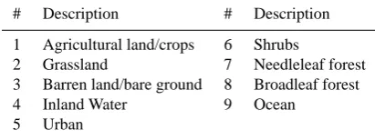
Table 2. Land use categories used in CHIMERE.

# Description # Description

1 Agricultural land/crops 6 Shrubs

2 Grassland 7 Needleleaf forest

3 Barren land/bare ground 8 Broadleaf forest

4 Inland Water 9 Ocean

5 Urban

3.3 Boundary and initial conditions

As a limited area model, CHIMERE requires chemical ini-tial and boundary conditions. The boundary conditions are three-dimensional fields covering the whole simulation pe-riod. These fields provide the concentrations of chemical species (gaseous and particulate) at the lateral and upper layers of the CHIMERE simulation domain. Some CTMs use tabulated vertical profiles derived from observational climatologies. Considering that observation-based boundary conditions are too restrictive in terms of available species, i.e. temporal and spatial coverage, CHIMERE gets its bound-ary conditions from global CTMs. The sensitivity study by Szopa et al. (2009) illustrates the importance of using a do-main that is large enough to minimise boundary effects and allow for recirculations within the CHIMERE domain.

To ensure the best possible simulation quality, a common practice is to use the nesting option of CHIMERE, with a coarse domain to provide the most consistent boundary con-ditions for the smaller nested domains. An example of such a configuration is displayed in Fig. 6 for a specific study in the Paris area with the horizontal resolution1x=5 km. The local simulation is nested into a larger domain with1x= 15 km, which itself is nested into a domain with1x=45 km. Only the largest domain makes use of external boundary con-ditions (Fig. 6).

Szopa et al. (2009) also investigated the sensitivity of the model to the temporal increment of the boundary con-ditions. They found that using a time-variable large-scale forcing improves the variability at the boundary of the

Domain description Purpose Domain scale ∆x×∆y nv ptop Reference

North-Atlantic Dust transport Hemispheric 1◦×1◦ 15 200 Menut et al. (2009a)

Europe Operational forecast Continental 0.5◦×0.5◦ 8 500 Rou¨ıl et al. (2009)

Europe Models comparisons Continental 25km×25km 9 200 Solazzo et al. (2012b)

North-America Models comparisons Continental 36km×36km 9 200 Solazzo et al. (2012b)

France Operational forecast National 0.15◦×0.1◦ 8 500 Rou¨ıl et al. (2009)

Western Europe Sensitivity study Continental 45km×45km 8, 9, 20 500 Menut et al. (2013)

Northern France Sensitivity study Regional 15km×15km 8, 9, 20 500 Menut et al. (2013)

Ile-de-France region Sensitivity study Urban area 5km×5km 8 500 Valari et al. (2011)

Table 1. Examples of some domains for which CHIMERE simulations have been performed, with their horizontal resolution,∆xand∆y, their number of vertical levels, nvand the domain top,ptop, in hPa.

# Description # Description

1 Agricultural land / crops 6 Shrubs

2 Grassland 7 Needleleaf forest

3 Barren land/bare ground 8 Broadleaf forest

4 Inland Water 9 Ocean

5 Urban

Table 2.Landuse categories used in CHIMERE

Fig. 6. Example of simulation domains for CHIMERE, and corre-sponding surface ozone concentrations maps. The largest domain (dx=45km) uses a global model climatology for boundary condi-tions, and forces itself the medium domain, dx=15km over the North of France, itself forcing the small domain, dx=5km, over the Paris area.

They found that using a time-variable large scale forcing

im-435

proves the variability at the boundary of the domain com-pared to the monthly average, but the magnitude of the sen-sitivity decreases towards the centre of the domain. Schere et al. (2012)confirmed this finding during the AQMEII in-tercomparison exercise. Colette et al. (2011)argued that the

440

selection of the large scale model had a larger impact than its temporal resolution.

Depending on the research projects that have been

con-ducted in the past, preprocessing tools have been imple-mented to build boundary conditions from a variety of

445

global models. The most widely employed is LMDz-INCA (Folberth et al. (2006)), for which a climatology (average monthly fields) is available on the CHIMERE website. Al-ternatively, the MOZART model was also used, for instance for the GEMS (Hollingsworth et al. (2008)), MACC II, and

450

AQMEII (Rao et al. (2011)) projects, and an interface with OsloCTM2 (Sovde et al. (2008)) was also developed for the CityZen project. For the specific case of mineral dust, the GOCART (Ginoux et al. (2001)) monthly average fields are also available. The current version of the model includes in

455

its namelist a series of flags in order to define which model is to be used for the following three groups of species: gases, dust aerosols, and non-dust aerosols. For each of them either climatological or time-varying fields can be used.

The initial conditions are a three-dimensional field

corre-460

sponding to the starting date of the simulation. The same global model fields used for boundary conditions can be used to initiate the simulation. If there are no global model fields available, it is also possible to start a simulation with zero concentrations for all species. In this case, the spin-up time

465

of the simulation has to be adjusted to the domain size: from a few days for a local domain to one month for a continen-tal domain (to take into account the long-range transport and possible recirculations).

4 Meteorology

470

CHIMERE is an off-line chemistry-transport model driven by meteorological fields, e.g., from a weather forecast model, such as WRF or MM5. CHIMERE contains a meteorologi-cal pre-processor that prepares standard meteorologimeteorologi-cal vari-ables to be read by the model core.

475

The input meteorological data are processed in two stages, as presented in Figure 7 . This choice constitutes a strength of the CHIMERE model: the user can use CHIMERE pro-viding only very basic meteorological variables: wind speed, temperature, humidity and pressure. In this case, a complete

480

suite of diagnostic tools for all other mandatory variables (turbulent fluctuations and fluxes) may be used. On the other

Fig. 6. Example of simulation domains for CHIMERE, and

corre-sponding surface ozone concentrations maps. The largest domain (dx=45 km) uses a global model climatology for boundary condi-tions, and forces itself the medium domain, dx=15 km, over the North of France, itself forcing the small domain, dx=5 km, over the Paris area.

domain compared to the monthly average, but the magni-tude of the sensitivity decreases towards the centre of the domain. Schere et al. (2012) confirmed this finding during the AQMEII inter-comparison exercise. Colette et al. (2011) argued that the selection of the large-scale model had a larger impact than its temporal resolution.

(8)

Fig. 7. Treatment of meteorological fields: two options are avail-able (i) using a meteorological dataset restricted to the mean pa-rameters (u,v,T,q,P, precipitation) and (ii) using a complete meteo-rological dataset that includes turbulent parameters.

hand, if the meteorological model provides all the necessary meteorological variables, the meteorological interface only interpolates data on the CHIMERE grid, with an hourly time

485

step. The diagnostic interface may also be used even if tur-bulent parameters are provided with the meteo model. The user can decide to bypass turbulent parameterisations of the input meteorological model and make use of the CHIMERE diagnostics in order to increase the consistency of the forcing

490

fields accross a range of input models.

The meteorological interface first transforms original vari-ables from any input spatial grid and temporal frequency onto standard variables given on the CHIMERE horizontal grid as hourly values. The operations performed include: horizontal

495

and temporal interpolation, wind vector rotation, temporal deaccumulation of precipitations, transformation from per-turbation and mean values to full values, etc. The vertical in-terpolation is performed at a later stage, since a higher verti-cal resolution might be required for the turbulence and fluxes

500

diagnostics. In the current CHIMERE version, meteorolog-ical interfaces are provided for ECMWF (ERA-INTERIM, IFS), WRF (Skamarock et al. (2007)) and MM5 models.

If not all required fields are provided, the pre-processor di-agnostic model is used. It takes meteorological variables and

505

transforms them into variables necessary for the CHIMERE core. These parameters are (i) the radiation attenuation, (ii) the boundary layer height, (iii) the friction velocity u∗, the aerodynamical resistance ra, the sensible heat flux Q0, the

Monin-Obukhov lengthLand the convective velocity w∗.

510

For the photochemistry, the cloud liquid water content is necessary to estimate the radiative attenuation. If rain water

or ice are available, they are added to the cloud water for the attenuation effects. Note that for gaseous species (such as HNO3) and aerosols calculations, additional parameters

re-515

lated to convective and large-scale precipitation are required for the scavenging.

Finally, and since most large-scale weather models do not include any ”urban parameterisation”, the possibility of cor-recting the wind speed in the surface layer (due to increased

520

roughness) in urban areas is offered. This will automatically be balanced by a vertical wind component calculated in the mass balance (see vertical transport below). This correction has however no effect at continental scale where the frac-tion of urban areas in the model grid cells are limited (see

525

Figure 5 for example, where the Paris city, a urban site, is not a ’dominant’ landuse for the corresponding cell). This ur-ban parameterisation has however a strong impact on urur-ban versions of the model, mostly for primary pollutants.

4.1 Diagnostic of turbulent parameters

530

The turbulent parameters may be read form the meteoro-logical driver or diagnosed in CHIMERE, as explained in Figure 7 . In case of a CHIMERE diagnostic, the following variables are calculated: the friction velocityu∗, the surface sensible heat fluxQ0, the vertical convective velocityw∗, the

535

boundary layer heighth, the bulk Richardson numberRiB,

the Monin-Obukhov lengthLand the vertical diffusivity pro-fileKz.

The friction velocity u∗ is used for the deposition and calculation of diffusivities. It is a particularly sensitive

pa-540

rameter for ozone in summer through the calculation of the aerodynamic resistance ra. Friction velocity is thus

sensi-tive to the land use type, which is critical to deposition. In large scale meteorological models, roughness lengths are of-ten too coarse for the implementation of high-resolution

de-545

position. Therefore an update of u∗is proposed following the

Louis et al. (1982)formulation which is particularly robust. We recommend to use this alternative formulation, no matter whether u∗ is available in the input fields, in order to have a deposition that is consistent with the high-resolution land

550

use.

u∗=

q C2

DNFm|U|2 (4)

with|U|the mean wind speed at 10 m above ground level,

Fmis theLouis et al. (1982)stability function andCDN the

momentum transfer coefficient as:

555

CDN=

k

ln

_z

z0m

(5)

withk=0.41 the Karman constant,zthe altitude where the wind speed|U|is known andz0m, the momentum roughness

length. The momentum stability function Fm is estimated

Fig. 7. Treatment of meteorological fields; two options are

avail-able: (i) using a meteorological dataset restricted to the mean pa-rameters (u, v, T , q, P ,precipitation) and (ii) using a complete me-teorological dataset that includes turbulent parameters.

Chemistry Aerosol Radiation and Transport) (Ginoux et al., 2001) monthly average fields are also available. The current version of the model includes in its name list a series of flags in order to define which model is to be used for the follow-ing three groups of species: gases, dust aerosols, and non-dust aerosols. For each of them either climatological or time-varying fields can be used.

The initial conditions are included in a three-dimensional field corresponding to the starting date of the simulation. The same global model fields used for boundary conditions can be used to initiate the simulation. If there are no global model fields available, it is also possible to start a simulation with zero concentrations for all species. In this case, the spin-up time of the simulation has to be adjusted to the domain size: from a few days for a local domain to one month for a conti-nental domain (to take into account the long-range transport and possible recirculations).

4 Meteorology

CHIMERE is an off-line chemistry-transport model driven by meteorological fields, e.g. from a weather forecast model, such as WRF or MM5. CHIMERE contains a meteorological preprocessor that prepares standard meteorological variables to be read by the model core.

The input meteorological data are processed in two stages, as presented in Fig. 7. This choice constitutes a strength of the CHIMERE model: the user can use CHIMERE providing only very basic meteorological variables such as wind speed,

temperature, humidity and pressure. In such a case, a com-plete suite of diagnostic tools for all other mandatory vari-ables (turbulent fluctuations and fluxes) may be used. On the other hand, if the meteorological model provides all the nec-essary meteorological variables, the meteorological interface only interpolates data on the CHIMERE grid, with an hourly time step. The diagnostic interface may also be used even if turbulent parameters are provided with the meteo model. The user can decide to bypass turbulent parameterisations of the input meteorological model and make use of the CHIMERE diagnostics in order to increase the consistency of the forcing fields across a range of input models.

The meteorological interface first transforms original vari-ables from any input spatial grid and temporal frequency into standard variables on the CHIMERE horizontal grid as hourly values. The operations performed include horizontal and temporal interpolation, wind vector rotation, temporal deaccumulation of precipitations, transformation from per-turbation and mean values to full values, etc. The vertical interpolation is performed at a later stage, since a higher vertical resolution might be required for the turbulence and fluxes diagnostics. In the current CHIMERE version 2013, meteorological interfaces are provided for ECMWF (ERA-INTERIM, IFS), WRF (Skamarock et al., 2007) and MM5 models.

If not all required fields are provided, the preproces-sor diagnostic model is used. It takes meteorological vari-ables and transforms them into varivari-ables necessary for the CHIMERE core. These parameters are (i) the radiation atten-uation, (ii) the boundary layer height, (iii) the friction veloc-ityu∗, (iv) the aerodynamical resistancera, (v) the sensible

heat fluxQ0, (vi) the Monin–Obukhov lengthLand (vii) the

convective velocityw∗.

For the photochemistry, the cloud liquid water content is necessary to estimate the radiative attenuation. If rain water or ice are available, they are added to the cloud water for the attenuation effects. Note that for gaseous species (such as HNO3) and aerosols calculations, additional parameters

re-lated to convective and large-scale precipitation are required for the scavenging.

Finally, and since most large-scale weather models do not include any “urban parameterisation”, the possibility of cor-recting the wind speed in the surface layer (due to increased roughness) in urban areas is offered. This will automatically be balanced by a vertical wind component calculated in the mass balance (see vertical transport below). This correction has however no effect at continental scale where the frac-tion of urban areas in the model grid cells are limited (see Fig. 5 for example, where the Paris city, an urban site, is not a “dominant” land use for the corresponding cell). This ur-ban parameterisation has however a strong impact on urur-ban versions of the model, mostly for primary pollutants.

(9)

4.1 Diagnostic of turbulent parameters

The turbulent parameters may be read from the meteorologi-cal driver or diagnosed in CHIMERE, as explained in Fig. 7. In the case of a CHIMERE diagnostic, the following vari-ables are calculated: the friction velocityu∗, the surface sen-sible heat fluxQ0, the vertical convective velocity w∗, the

boundary layer heighth, the bulk Richardson numberRiB,

the Monin–Obukhov length L, and the vertical diffusivity profileKz.

The friction velocity u∗ is used for the deposition and calculation of diffusivities. It is a particularly sensitive pa-rameter for ozone in summer through the calculation of the aerodynamic resistance ra. Friction velocity is thus

sensi-tive to the land use type, which is critical to deposition. In large-scale meteorological models, roughness lengths are of-ten too coarse for the implementation of high-resolution de-position. Therefore an update ofu∗is proposed following the Louis et al. (1982) formulation, which is particularly robust. We recommend using this alternative formulation, no matter whetheru∗ is available in the input fields, in order to have a deposition that is consistent with the high-resolution land use.

u∗=

q

C_DN2 Fm|U|2, (4)

with|U|the mean wind speed at 10 m above ground level,

Fmis the Louis et al. (1982) stability function andCDN the

momentum transfer coefficient as

CDN=

k

ln

z z0m

, (5)

withk=0.41 the Karman constant,zthe altitude where the wind speed|U|is known andz0m, the momentum roughness

length. The momentum stability functionFmis estimated

ac-cording to the bulk Richardson number,Rib, value.Rib is

estimated at each altitudezas

Rib(z)= g z θv(z)

θv(z)−θv(z0)

|U (z)|2 , (6)

with g=9.81 m2s−2 the gravitational acceleration and θv

the virtual potential temperature in Kelvin. – In unstable cases, ifRib<0:

Fm=1−

2b Rib

1+3b c C_DN2 .

r _z

z0m p

|Rib|

. (7)

– In stable cases, ifRib>0:

Fm=

1 1+√2b Rib

1+d Rib

(8)

with the constant b=c=d=5. In the neutral case, i.e

Rib=0,Fm=1.

The surface sensible heat flux,Q0, is used to computew∗

and therefore mixing, and the height of the boundary layer. In fact, only the virtual heat flux is required, which can be re-computed from an empirical formula (Priestley, 1949) using temperatures in the first model layers. However, this formula is not very accurate and it is strongly advised to use heat fluxes from the meteorological model, if available. If the sur-face sensible heat fluxQ0is provided by the meteorological

model, it is directly used for the computation of the convec-tive velocityw∗:

w∗= g Q0h

ρ Cpθv !1/3

, (9)

wherehis the convective boundary layer height,Cpthe

spe-cific heat of air at constant pressure, andθvthe mean virtual

potential temperature in the first model vertical level. The Monin–Obhukov length is estimated as

L=−θvu

3

∗ k g Q0

. (10)

The boundary layer height (h) is derived from different formulation, depending on the atmospheric static stability. When stable, i.e whenL >0, his estimated as the altitude when the Richardson number reaches a critical number here chosen asRic=0.5, following Troen and Mahrt (1986).

In unstable situations (i.e. convective),his estimated us-ing a convectively-based boundary layer height calculation. This is based on a simplified and diagnostic version of the approach of Cheinet and Teixeira (2003) which consists in the resolution of the (dry) thermal plume equation with dif-fusion. The in-plume vertical velocity and buoyancy equa-tions are solved and the boundary layer top is taken as the height where calculated vertical velocity vanishes. Thermals are initiated with a non-zero vertical velocity and potential temperature departure, depending on the turbulence similar-ity parameters in the surface layer.

Once the depth of the boundary layer is computed, ver-tical turbulent mixing can be applied by following the K-diffusion framework, which follows the parameterisation of Troen and Mahrt (1986), but without counter-gradient term. In each model column, the diffusivity coefficient profileKz

(m2s−1) is calculated as

Kz=kws

z h

1−z

h

2

(11) wherewsis a vertical scale given by similar formulas:

– In the stable case (when the surface sensible heat flux is negative)

ws=

u∗