Geosci. Model Dev., 7, 211–224, 2014 www.geosci-model-dev.net/7/211/2014/ doi:10.5194/gmd-7-211-2014
© Author(s) 2014. CC Attribution 3.0 License.
Geoscientific
Model Development
Open Access
An improved parameterization of tidal mixing for ocean models
A. Schmittner and G. D. Egbert
College of Earth, Ocean and Atmospheric Sciences, Oregon State University, Corvallis OR, USA
Correspondence to: A. Schmittner ([email protected])
Received: 13 August 2013 – Published in Geosci. Model Dev. Discuss.: 4 September 2013 Revised: 13 December 2013 – Accepted: 17 December 2013 – Published: 28 January 2014
Abstract. Two modifications to an existing scheme of tidal mixing are implemented in the coarse resolution ocean com-ponent of a global climate model. First, the vertical distribu-tion of energy flux out of the barotropic tide is determined using high resolution bathymetry. This shifts the levels of mixing higher up in the water column and leads to a stronger mid-depth meridional overturning circulation in the model. Second, the local dissipation efficiency for diurnal tides is assumed to be larger than that for the semi-diurnal tides pole-ward of 30◦. Both modifications are shown to improve agree-ment with observational estimates of diapycnal diffusivities based on microstructure measurements and circulation in-dices. We also assess impacts of different spatial distribu-tions of the barotropic energy loss. Estimates based on satel-lite altimetry lead to larger diffusivities in the deep ocean and hence a stronger deep overturning circulation in our climate model that is in better agreement with observation based es-timates compared to those based on a tidal model.
1 Introduction
Mixing processes on scales smaller than the grid cell size substantially influence the resolved large-scale flow in global, coarse resolution general circulation ocean models (Bryan and Lewis, 1979) with implications for heat and tracer fluxes, climate and biological productivity. Vertical, or more accurately, diapycnal mixing is particularly important in determining the strength of the global meridional overturn-ing circulation (MOC; Bryan, 1987). Duroverturn-ing the last decade progress has been made in better understanding processes that lead to diapycnal mixing. One such process is flow, of-ten due to tides, over rough topography that generates inter-nal waves. Wave breaking can lead to turbulence and mixing. Parameterizations of tidal mixing have been developed (St
Laurent et al., 2002) and successfully implemented in various ocean general circulation models (Jayne, 2009; Montenegro et al., 2007; Saenko, 2006; Saenko and Merryfield, 2005; Schmittner et al., 2005; Simmons et al., 2004b).
Most of these studies use a two-dimensional map of en-ergy loss by the external (surface) tide based on the hy-drodynamic, barotropic tide model of Jayne and St Lau-rent (2001; JS01), who parameterize the internal wave drag as a linear function of tidal velocities modulated by bottom roughness (Fig. 1). Quadratic bottom drag is also included in JS01, but this effect is important only in the shallow ocean along continental margins where tidal velocities are large. In JS01 almost all (1.41 out of a total of 1.51 TW) dissipation due to bottom drag occurs above 178 m depth, whereas all (1.99 TW) dissipation due to internal wave drag occurs be-low 178 m (Table 1). Thus bottom drag has little effect on the large-scale circulation, which is controlled by mixing in the thermocline.
Typically coarse resolution climate models have smoothed bathymetry and do not resolve many narrow features of the real sea floor such as island chains or sea mounts. Here we show that using a global two-dimensional map of the energy flux averaged on the coarse resolution climate model grid, as done in previous studies, can bias the depths where mixing takes place, with impacts on the simulated MOC. One goal of this study is to develop a modified scheme that considers re-alistic, high-resolution bathymetry, and to evaluate its effects on the distribution of mixing and simulated MOC.
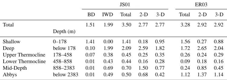
Table 1. Energy flux (TW) out of the barotropic tide estimated by JS01 and ER03 for different depth ranges. Note that JS01 provides separation between bottom drag (BD) and internal wave drag (IWD), whereas ER03 does not. The subcolumns on the left are based on calculations on the original 1/2◦grid for JS01 and on a 1/6◦grid for ER03. The subcolumns on the right denote fluxes averaged on the climate model grid without (2-D) and with (3-D) the consideration of subgrid-scale bathymetry. The depth levels are based on the climate model grid.
JS01 ER03
BD IWD Total 2-D 3-D Total 2-D 3-D
Total 1.51 1.99 3.50 2.77 2.77 3.28 2.92 2.92
Depth (m)
Shallow 0–178 1.41 0.00 1.41 0.18 0.95 1.56 0.27 0.88
Deep below 178 0.10 1.99 2.09 2.59 1.82 1.72 2.65 2.04
Upper Thermocline 178–458 0.07 0.38 0.45 0.25 0.35 0.26 0.24 0.29 Lower Thermocline 458–858 0.01 0.43 0.44 0.16 0.28 0.09 0.18 0.16 Mid-Depth 858–2383 0.01 0.69 0.70 1.50 0.77 0.24 0.85 0.45 Abbys below 2383 0.01 0.49 0.50 0.68 0.42 1.12 1.37 1.14
the barotropic tide (E) is dissipated locally for all tidal con-stituents. Although this assumption may be warranted for the semi-diurnal tides over most of the globe (equatorward of 70◦; Simmons et al., 2004a), it may not be appropriate for diurnal tides, which are trapped to topography poleward of 30◦, and may thus be relatively more effective at driving local mixing. A second objective of this paper is to consider this fundamental difference between the tidal constituents and evaluate its effects on the distribution of mixing and MOC.
Alternative parameterizations of E have been proposed (Nycander, 2005; Zaron and Egbert, 2006) and shown to lead to different spatial distributions (Green and Nycander, 2013). Inversions of satellite altimeter data do not rely on specific parameterizations and thus provide independent, empirical estimates of E (Egbert and Ray, 2003; ER03; Fig. 1). As shown in detail in Egbert and Ray (2001) averages ofEover large (500–1000 km scale) patches of open ocean are con-strained well by altimetry data, while finer scales (especially near coastlines or in areas of rough topography) are more poorly determined (Zaron and Egbert, 2006). Thus the de-tailed spatial distribution ofEis unknown. A third objective of our study will be exploration of these uncertainties and their effects on ocean mixing and the simulated MOC.
2 Methods
2.1 Model description
The University of Victoria (UVic) Earth System Model (Weaver et al., 2001), here we use version 2.8 with pa-rameters as reported in Schmittner et al. (2008), has been widely used in climate and paleoclimate applications. It includes a three-dimensional ocean circulation compo-nent, dynamic-thermodynamic sea ice, a one-layer, two-dimensional energy–moisture balance atmosphere, as well as land (Meissner et al., 2003) and ocean (Schmittner et al.,
2008) biogeochemistry. Wind velocities are prescribed us-ing a repeatus-ing mean annual cycle of monthly data from the NCEP (National Centers for Environmental Prediction) re-analysis. All model components have a resolution of 3.6◦ in longitude×1.8◦ in latitude, and the ocean has 19 verti-cal levels with 50 m grid spacing near the surface increas-ing to 500 m at 5.5 km depth. Due to the simple energy– moisture balance atmospheric model and the prescribed wind velocities, the model does not simulate weather and its inter-nal variability on interannual to decadal timescales is much smaller than observed. The UVic model is computationally efficient and it includes the tidal mixing parameterization of St. Laurent et al. (2002; S02) as implemented by Simmons et al. (2004b), which calculates the spatially varying diapycnal diffusivity according to
kv=kbg+
0ε
N2, (1)
wherekbg=0.15×10⁻⁴m2s−1is the global constant
back-ground diffusivity,N is the buoyancy frequency,0=0.2 is the mixing efficiency and the turbulent energy dissipation rate
ε=qE(x, y)F (z, H )
ρ (2)
is a function of the local tidal dissipation efficiencyq, the energy flux out of the barotropic tideE(x, y), which depends on longitudexand latitudey, densityρ, and
F (z, H )= e
−(H−z)/ζ
A. Schmittner and G. D. Egbert: An improved parameterization of tidal mixing 213
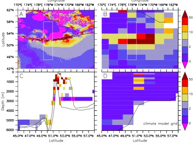
Fig. 1. Logarithm of total energy flux out of the barotropic tideE(W m−2)estimated from satellite altimetry (ER03, left) and a tide model (JS01, right). Top: data on high resolution grid. Bottom: data averaged on climate model grid. Negative values for ER03 are shown in white and have been set to zero on the climate model grid.
that turbulence is generated through tidal currents interact-ing with topography and decays exponentially above the sea floor. The fraction ofE that is locally dissipated is repre-sented byq. In the original S02 schemeq=0.33, with the remaining two-thirds of the energy assumed to radiate away and dissipate at an unknown location, effectively contribut-ing tokbgin Eq. (1).N2is limited to be larger than 10−8s−1
and kv may not exceed 10−2m2s−1, in order to prevent numerical instabilities. Diffusivities in the Southern Ocean south of 40◦S and below 500 m are limited to values greater than 10−4m2s−1in order to account for observations of en-hanced mixing there (Naveira Garabato et al., 2004). Note that Eq. (1) considers explicitly only tidally driven mixing, whereas all other sources of mixing are folded intokbg.
2.2 Energy flux from the barotropic tide
We use two-dimensional maps of energy lossesETC2-D(x, y)
from the surface tide from two sources. First, the four ma-jor tidal constituents (TCs), the semidiurnal lunar and so-lar tides, M2 and S2, respectively, and the diurnal K1 and O1 tides, estimated from assimilation of satellite altimetry data into a 1/6◦×1/6◦hydrodynamic model as in ER03 are used. Second,E simulated by a barotropic tide model with parameterized internal wave drag, and without data assimila-tion at 1/2◦×1/2◦resolution for a larger set of constituents
(JS01) as described in Montenegro et al. (2007) are used. Figure 1 shows the total (sum over all TCs) energy flux. The general spatial patterns are similar between JS01 and ER03 showing regions of high dissipation associated with major topographic features such as the Mid-Atlantic Ridge and the Hawaiian Islands chain. However, there are also im-portant differences in the maps, which are consistent with their derivation. The empirical map from ER03 is smoother, less sharply focused on specific features, and has generally higher values in the interior of the ocean basins. Energy fluxes in JS01 are more concentrated along the margins and over rough topography, consistent with this model’s parame-terization of internal wave drag.
Fig. 2. Horizontally integrated energy loss from the barotropic tide for ER03 (E) and JS01 (J) as a function of depth. The climate model’s vertical grid of 19 levels is used for the depth axis. High resolution levels below the deepest model level are added to the bottom box. Shown are original data using high horizontal resolu-tion (blue) and data regridded on the climate model grid with (red) and without (black) subgrid-scale bathymetry scheme. The surface (50 m) values for the blue lines are 1.3 TW for bothEandJ.
Averaging on the UVic climate model grid and masking out grid points that are designated land in the climate model leads to a reduction of the global energy flux. Note that this depends on the climate model grid and resolution used. In our version of the the UVic model this reduction is larger for JS01 (0.73 TW) since more energy is lost around the conti-nental margins compared with ER03 (0.36 TW). Thus mod-els using ER03 have slightly more global energy available for mixing (2.92 TW) than those using JS01 (2.77 TW). ER03 results in negative dissipation estimates in certain regions (white areas in top left panel of Fig. 1). Although conver-sion from baroclinic to barotropic tides could occur in the real ocean (as it does in the model of Simmons et al., 2004a) for our parameterization this would result in unphysical neg-ative diffusivities. Therefore, after averaging on the model grid we set all negative values to zero.
Simmons et al. (2004a), using a 10-layer global model with 8 tidal constituents, estimate that 1.34 TW is converted from the barotropic tide to internal waves, significantly less than ER03 and JS01. This discrepancy supports the suspi-cion of Simmons et al. (2004a) that their results are biased low in regions such as the Mid-Atlantic Ridge, where con-version increases with increased resolution as more higher mode waves are included. Arbic et al. (2010) show that even at 1/12◦ horizontal resolution (the highest currently possi-ble) global baroclinic models resolve well only the two low-est modes, whereas mode numbers greater than 10 are not resolved at all.
2.3 Innovations
We introduce two innovations to the S02 scheme. First, we consider diurnal and semi-diurnal tidal constituents sepa-rately, allowing for differences in wave propagation, and sec-ond, we employ a new scheme for subgrid-scale bathymetry, to allow a more realistic vertical distribution of tidal mixing. With these extensions the total energy dissipation rate (Eq. 2)
ε= 1
ρ
H X
z0>z X
TC
qTCETC(x, y, z0)F (z, z0) (4)
is expressed as a sum of contributions from TC (i.e., M2, S2, K1, O1) and the treatment of subgrid scale bathymetry from all levelsz0 belowzand above the climate model sea floor
H.F (z, z0)in Eq. (4) is the vertical decay function in Eq. (3) whereHhas been replaced byz0.
2.3.1 Semi-diurnal and diurnal tidal constituents
Since there are no free gravity waves over a flat bottom pole-ward of the critical latitude (i.e., for subinertial frequencies,
ω<f; e.g., Wunsch, 1975) we assume complete local dissi-pation of tidal energy for the diurnal tides poleward of 30◦ (qD=qK1=qO1=1) and incomplete local dissipation for
the semi-diurnal tides (qM2=qS2=0.33) for ER03. This
re-finement is not possible for JS01, as only total dissipation maps were available (and thus we takeq=0.33 for all TCs). A sensitivity experiment with ER03 andq=0.33 for all TCs quantifies the effects of qD on the results. For ER03 the
global dissipation for the different tidal constituents is 2.42, 0.40, 0.30, and 0.16 TW for M2, S2, K1, and O1, respec-tively. Below 178 m the diurnal tides K1 and O1 contribute about 16 % to the total dissipation at high resolution, whereas this fraction increases to 24 % if averaged on the model grid using the subgrid-scale bathymetry scheme described below and to 27 % if the subgrid-scale scheme is not used.
2.3.2 Subgrid-scale bathymetry
A. Schmittner and G. D. Egbert: An improved parameterization of tidal mixing 215
Fig. 3. Illustration of subgrid-scale scheme using the Aleutian Islands chain as an example. (A): energy fluxE(10−3W m−2)out of the K1 barotropic tide from ER03. (B): as (A) but averaged on the climate model grid. The white boxes in (A) and (B) denote a section of one climate model grid box zonal width (3.8◦) shown in (C) and (D). Black lines in (A) and (B) show the 500 m isobath from a high resolution bathymetric data set (etopo20) and the model, respectively. (C):Efrom (A) averaged on a 1/3◦horizontal grid of etopo20 at the corresponding levels of the climate model. On this grid there is only one level of nonzero data. Displayed are zonally averaged values ofE
within the white box shown in panel (A), which leads to some latitudes having more than one nonzero values in the figure. In cases where the deepest climate model grid box is shallower than the deepest high resolution bathymetryEis shifted up on the level of the deepest climate model grid box (e.g., at 56◦N). Lines show the zonal maxima and minima of the high resolution bathymetry. (D):Efrom (C) horizontally averaged on the climate model grid. Model bathymetry is shown as the black line. Note that the sum over all vertical levels in (D) equals (B).
Edwards, 1986). Next we assignE (on the high-resolution grid) to a vertical climate model level that corresponds to the actual (high-resolution) sea floor (Fig. 3c). (We use veloc-ity grid levels since the UVic model uses a staggered grid and diffusivities and tracer fluxes are calculated on the ve-locity grid, which corresponds to the grid box boundaries of the tracer grid.) High-resolution bathymetry below the deep-est model grid box is assigned to the deepdeep-est model grid box. This leads to a three-dimensional (3-D) map at high horizontal (0.3◦×0.3◦) and coarse vertical (the 19 climate model levels) resolution, where only one vertical level has a value different from zero. Subsequently this field is av-eraged horizontally onto the coarse resolution model grid and negative values are set to zero. This results in a three-dimensional field ETS(x, y, z) on the climate model grid,
which is used in Eq. (4) to computeε. Note thatETC2-D(x, y)= H
P
z0=0
ETC(x, y, z0); i.e., the total amount of energy available
for mixing remains the same, but is distributed over a range of depths.
2.4 Numerical experiments
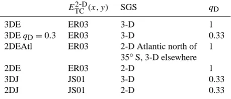
In the following we present results from six different exper-iments (Table 2). Acronyms beginning with 3-D indicate the use of the subgrid-scale bathymetry scheme, whereas exper-iment acronyms starting with 2-D do not. The subsequent letter (EorJ) indicates which estimate for the barotropic en-ergy flux is used (ER03 vs. JS01). One experiment has been performed, in which the 3-D scheme is used everywhere ex-cept in the Atlantic north of 35◦S, where the 2-D scheme is
used (2DEAtl). This will allow us to quantify the influence of mixing changes in the Atlantic only on the global MOC. Ex-periment 3DEqD=0.3 explores the effects of different
Table 2. Acronyms of climate model experiments performed with different estimates of the barotropic tide energy fluxETC2-D(x, y), with (3-D) or without (2-D) the subgrid-scale (SGS) bathymetry scheme, and the value for the local dissipation efficiency of the di-urnal tidesqD.
E2TC-D(x, y) SGS qD
3DE ER03 3-D 1
3DEqD=0.3 ER03 3-D 0.33
2DEAtl ER03 2-D Atlantic north of 1 35◦S, 3-D elsewhere
2DE ER03 2-D 1
3DJ JS01 3-D 0.33
2DJ JS01 2-D 0.33
All simulations have been run for 4000 yr to equilibrium and results averaged over the last 10 yr are presented. In or-der to assess the different schemes we will compare resulting diffusivities with estimates based on observations. However, stratification evolves in the simulations and will affect dif-fusivities. In order to separate the effect of variations inN2
from those due to the subgrid-scale scheme andEestimates we have also conducted short (10 d) simulations initialized from identical initial conditions of zero velocities and tem-perature and salinity from observations. This leads to essen-tially identicalN2close to observations. We will show time averaged results from these short runs as thick lines and re-sults from equilibrium (at model year 4000) as thin lines in Figs. 5, 9, 10, 11, and 12.
3 Results
3.1 Effects on the vertical distribution of energy fluxes
RegriddingEon the climate model grid without considering subgrid-scale bathymetry (black vs. blue lines in Fig. 2 and 2-D vs. “Total” columns in Table 1) leads to a shift of dissi-pation from the upper to the deep ocean. Below 858 m depth dissipation increases by 82 (JS01) and 63 % (ER03), whereas this bias is strongly reduced (to<1 % and 17 %) if subgrid-scale bathymetry is considered (3-D columns in Table 1). The root mean of squared errors RMSE calculated from the horizontally integrated vertical profiles shown in Fig. 2 re-duces dramatically from 0.19 TW for both 2-D schemes to 0.09 (3DJ) and 0.10 TW (3DE), strong evidence that the ver-tical distribution of the energy transfer is considerably more realistic for the 3-D experiments.
3.2 Effects on mixing and circulation
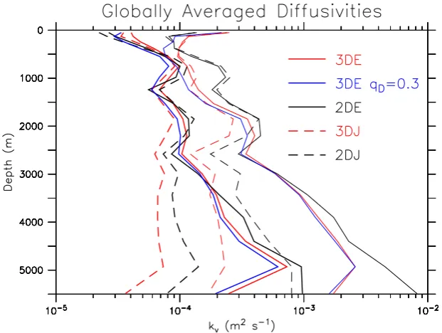
ER01 dissipates more energy in the abyssal plains than JS01 as illustrated in Fig. 4 for the North Pacific. Our parameter-ization of subgrid-scale bathymetry (3-D experiments) leads to a considerable amount of dissipation at much shallower
depths than the model sea floor in regions of narrow and steep topographic features (Figs. 3d, 4) and generally to a shift of mixing higher up in the water column compared with the 2-D experiments (Figs. 2–5). This is true for both ER01 and JS01. However, global mean diffusivities are generally lower in the 3-D scheme (Fig. 5). In 3DE, e.g., it is 1.3×10⁻⁴m2s−1 at model day 10 compared with 1.6×10⁻⁴m2s−1 in 2DE despite identical global mean dissipation andN2. This fol-lows from Eq. (1), according to which an upward shift in dissipation leads to a decrease in global meankvsinceN2is larger at shallower depth andkvis proportional to dissipation
εweighted by the inverse ofN2.
For the same reason (more dissipation at shallower depths) global mean diffusivities for JS01 are smaller (6.1×10⁻⁵ and 8.0×10⁻⁵m2s−1 for 3DJ and 2DJ, respectively) than those for ER03. Whereas ER03 and JS01 result in similar globally averaged diffusivities in the upper ocean, ER03 pro-duces substantially larger values in the deep ocean (Fig. 5) consistent with more dissipation there (Figs. 1, 2).
The effect ofqDon globally averaged diffusivities is small.
In experiment 3DEqD=0.3 the mean is 1.1×10⁻⁴m2s−1
and horizontal averages are slightly smaller at all depths compared with experiment 3DE.
As the experiments approach equilibrium N2 decreases and generally is lower than observed below about 1 km depth (not shown). This leads to higher diffusivities in the deep ocean at equilibrium compared with model day 10 (Fig. 5).
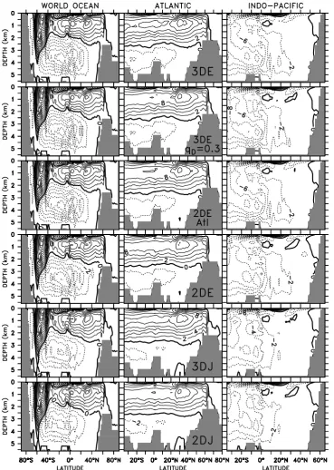
The equilibrium MOC is similar in all experiments (Fig. 6). However, the 3-D experiments simulate a slightly stronger (∼10 %) Atlantic MOC (AMOC) and higher rates of Circumpolar Deep Water (CDW) inflow into the Indian and Pacific oceans (Table 3). This may be surprising since global diffusivities were smaller in these experiments. How-ever, shifting mixing to shallower depth leads to more mixing in the thermocline, which is more important for the circula-tion than mixing in the weakly stratified bottom layers.
The sensitivity experiment with the 2-D scheme in the At-lantic (2DEAtl) and 3-D elsewhere shows bottom water cir-culation corresponding to the local mixing scheme; that is AABW in the Atlantic is identical to 2DE, whereas CDW flow into the Indian and Pacific oceans is identical to 3DE. However, the AMOC is in between experiments 2DE and 3DE, indicating that the AMOC increase in experiment 3DE compared with 2DE is about equally caused by local changes in mixing in the Atlantic as well as remote changes else-where.
A. Schmittner and G. D. Egbert: An improved parameterization of tidal mixing 217
Fig. 4. Effect of the subgrid-scale parameterization on vertical diffusivities along 178◦W in the North Pacific. The northern part of the section corresponds to the one shown in Fig. 3. All experiments were initialized from observations for temperature and salinity and integrated for 10 d, which leads to almost identicalN2.
Fig. 6. Meridional overturning stream function in Sverdrups (1 Sv = 106m3s−1)at equilibrium (model year 4000) for the global (left), the Atlantic (center), and the Indo-Pacific (right) for experiments (from top to bottom) 3DE, 3DEqD=0.3, 2DE Atl, 2DE, 3DJ, and 2DJ.
Isolines are shown every 2 Sv with positive (negative, dashed) values indicating clockwise (counter-clockwise) flow.
The effect of complete local dissipation of tidal energy for the diurnal tides (3DE vs. 3DEqD=0.3) is small. The
largest effect is simulated for the AMOC, which increases by 0.8 Sv.
3.3 Comparison with observation-based estimates
3.3.1 Circulation
A. Schmittner and G. D. Egbert: An improved parameterization of tidal mixing 219
26.5◦N, and the deep overturning, which are outside the
ob-servational error estimates for all experiments. Most exper-iments are within the observational error estimates for the other indices, with the exception of experiments 2DJ and 3DJ, which are inconsistent with the CDW flow into the Pa-cific as well. The RMSE indicates that experiments using ER03 are slightly better compared with JS01 based on the six indices considered. Including total local dissipation for diurnal tides poleward of 30◦improves the agreement with the observed circulation indices slightly, as indicated by the smaller RMSEs for experiment ER03 compared with experi-ment ER03qD=0.3.
In Table 3 we use only a subset of indices based on a global inversion of World Ocean Circulation Experiment data from the 1990s by Lumpkin and Speer (2007) and observational estimates of the AMOC at 26.5◦N from the RAPID
pro-gram (McCarthy et al., 2012). The choice of indices is sub-jective but based on a set that minimizes redundancy and cross-correlation. All experiments underestimate the AMOC both at 26.5◦N and at 32◦S. The fact that the differences between model and observations is larger at 26.5◦N than at 32◦S suggests that all experiments underestimate upwelling within the Atlantic between those latitudes. Elevated levels of mixing due to the subgrid-scale bathymetry within the At-lantic (2DE Atl vs. 2DE) and outside of the AtAt-lantic (3DE vs. 2DE Atl) contribute equally (0.6 Sv) to the increased AMOC at 26.5◦N between experiments 3DE and 2DE.
Overall, the simulated circulation of experiment 3DE ap-pears to fit best with observational circulation indices as indi-cated by the lowest RMSE of all experiments. However, the circulation is influenced by many factors other than vertical diffusivities; e.g., horizontal diffusivities, surface and bottom buoyancy and momentum forcing, and model bathymetry. Thus better agreement with observational estimates of circu-lation alone is no proof that one particular parameterization is superior. In the following we attempt to assess the simu-lated diffusivities and resulting heat fluxes and heat flux con-vergence using observational estimates based on microstruc-ture measurements. Differences between the 2-D and 3-D ex-periments are presumably the largest in regions of narrow bathymetric features that are unresolved in the model. Mi-crostructure measurements are few and far between but we have found data from the Hawaiian and Kuril island chains and elsewhere, which will be discussed next.
3.3.2 Hawaiian Ridge
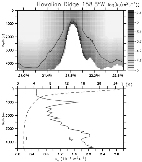
Measurements along the Hawaiian Ridge show large spatial and temporal variability. In order to calculate spatial aver-ages that correspond to the climate model grid scale we have to extrapolate the measurements. We use empirical formu-las as a function of height above the sea floor and distance from the ridge developed previously (Klymak et al., 2006). Resulting diffusivities for the Kauai Channel are high over the ridge and close to the sea floor (upper panel in Fig. 7)
Fig. 7. Estimates ofkvbased on microstructure observations from the Hawaiian Ridge during the HOME experiment. Top: extrap-olation on a typical climate model grid box of 1.8◦ meridional width using Eq. (2) of Klymak et al. (2006) applied to a section at 158.8◦W (Kauai Channel). A 1 min grid for the bathymetry and a vertical resolution of 100 m is used. Solid lines show contours at 10−3and 10−4m2s−1. Bottom: horizontally averaged profiles of
kv (solid) and climatological temperature (dashed; from WOA05, Locarnini et al., 2006) used to calculate heat fluxes.
Table 3. Ocean circulation indices in Sverdrups. “Mid global” denotes the strength of the mid-depth global meridional overturning cell. In the model it was calculated as the global maximum stream function below 400 m and north of the Equator. “Deep global” is the deep overturning cell calculated as the (negative) minimum of the global stream function below 1.5 km depth. “AMOC 32◦S” is the maximum stream function below 300 m in the Atlantic at 32◦S, “AABW Atl” is the (negative) minimum stream function in the Atlantic below 1 km at 35◦S. CDW represents inflow of Circumpolar Deep Water in the Indian and Pacific oceans at 32◦S. The first row shows independent estimates from an inverse model solution that uses observations (first 5 columns; Lumpkin and Speer, 2007; mid and deep global from their Fig. 2; others from Fig. 4) and, in the column labeled AMOC 26◦N observational estimates from the RAPID array. RAPID transport time series data were downloaded data from http://www.rapid.ac.uk/rapidmoc on 26 July 2013. Eight annual means were calculated from April 2004 to March 2012, as in McCarthy et al. (2012) but with one additional year. The value of 17.5 Sv reported in the table is the average over all eight years, the error estimate represents the standard deviation of the annual values. Bold numbers are within the observational error estimates and underlined and italic numbers are the best and worst matches for that particular index, respectively. The last column (RMSE) presents the root mean of squared errors of the other columns in Sverdrups.
deep AMOC AABW CDW CDW AMOC
global 32◦S Atl Ind 32◦S Pac 32◦S 26.5◦S RMSE
obs 20.9±6.7 12.0±3.1 5.6±3.0 9.2±2.7 11.0±5.1 17.5±2.0
3DE 14.0 10.6 4.2 5.2 7.4 11.3 4.5
3DEqD=0.3 14.0 9.8 4.1 5.1 7.1 10.6 4.7
2DEAtl 14.1 9.9 3.8 5.2 7.4 10.7 4.6
2DE 12.5 9.3 3.8 4.8 6.6 10.1 5.4
3DJ 8.6 10.8 2.9 5.8 5.3 11.4 6.3
2DJ 9.2 9.6 3.0 5.3 5.5 10.2 6.4
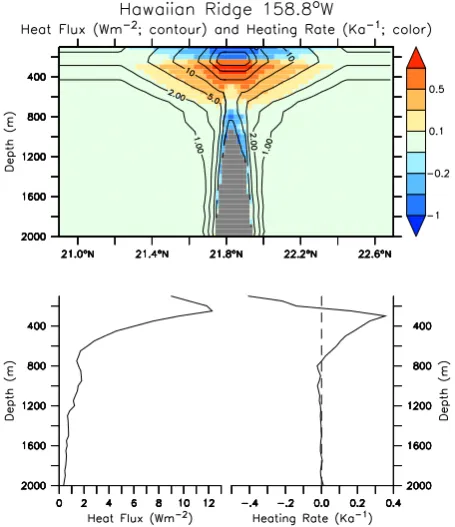
Fig. 8. As Fig. 7 but for the diffusive vertical heat flux (contour lines at 1, 2, 5, 10, 20, 30, and 40 W m−2shown in the upper panel) and heat flux convergence (color; units are Kelvin per year). Bottom panels show horizontally averaged values.
The details of these distributions depend on the local bathymetry. In order to get a rough uncertainty estimate we calculated diffusivities along three sections across the
Hawaiian Ridge, at 158.8, 162.6, and 166.5◦W using the same formulae (Klymak et al., 2006) based on observa-tions from the Kauai Channel (158.8◦W) and French Frigate Shoals (166.5◦W). Resulting horizontally averaged diffusiv-ities show relatively constant values between 5×10⁻⁵m2s−1 at the surface and 2×10⁻⁴m2s−1at 4 km depth (Fig. 9). All experiments overestimate the observed vertical variations. However, the 3-D experiments show larger values in the up-per ocean and smaller values at depth and are clearly in better agreement with the observations than the 2-D experiments.
Averaged heat fluxes based on the observations show max-ima of∼8 W m−2around 200 m and rapidly decreasing val-ues below that, whereas none of the experiments predicts a pronounced subsurface maximum and all experiments under-estimate heat fluxes in the upper 1 km (Fig. 10). Observed heating rates show maxima between 200 and 600 m consis-tent with the experiments. Heat fluxes in the 3-D experiments are in better agreement with the observation-based estimates for the short runs, whereas heating rates are not much differ-ent between the experimdiffer-ents.
3.3.3 Kuril Straits
A. Schmittner and G. D. Egbert: An improved parameterization of tidal mixing 221
Fig. 9. Comparison of simulated (lines)kv with observations (symbols) for Hawaii. Lines in main panel are horizontal averages of the nonwhite grid points in the inset maps. Both 10 d (thick) and equilibrium (model year 4000, thin) solutions are shown. Dotted line indicates the model’s background diffusivity. Insets show horizontal maps of simulated diffusivities at 1 km depth. Contour lines show the 3 km isobath from a 20 min resolution data set. Observational estimates were averaged over 2.7◦of latitude in order to correspond to the latitudinal averaging of the climate model results (see insets); 2.7◦was chosen because it is the average latitudinal width of the nonwhite model grid points.
lower values. Using a smaller value for the local dissipa-tion efficiency for the diurnal tides (qD=qK1=qO1=0.33)
leads to similar profiles for 3DE and 3DJ suggesting that the assumption of complete local dissipation (qD=1) of energy
from the diurnal tides in experiment 3DE is the most impor-tant difference between the experiments 3DE and 3DJ here. Better agreement with observations of experiment 3DE with
qD=1 compared withqD=0.33 supports the idea that most
energy extracted from the diurnal barotropic tide around the Kuril Islands is dissipated locally.
3.3.4 Other microstructure observations
Observations from elsewhere are not as clear in distinguish-ing between the different experiments. ER03 experiments predict higher diffusivities in the deep Brazil Basin, which appear to be in better agreement than JS01 (Fig. 12). Be-tween 2 and 3 km depth experiment 3DE is superior to 2DE but below∼4 km depth experiment 2DE fits the observations better. All experiments underestimate diffusivities between 1 and 2 km depth. Over the Mid-Atlantic Ridge at 37◦N the 3-D experiments match better elevated diffusivities at the base of the thermocline between 1 and 1.5 km depth than the 2-D experiments.
Fig. 10. As Fig. 9 but for the heat flux and heat flux convergence.
4 Discussion and conclusions
Fig. 11. Comparison of simulated (lines)kvwith observations for the Kuril Straits (151◦E, 46.5◦N). Green arrows denote the range of diffusivity estimates from microstructure measurements during spring and neap tides (Itoh et al., 2010, 2011) and the blue square shows an estimate of the time mean (Nakamura et al., 2006). The observational estimates represent the upper 500 m of the water col-umn. The blue line is experiment 3DE with reduced local dissi-pation of diurnal tide energy (qD=qK1=qO1=0.33). Both 10 d
(thick) and equilibrium (model year 4000, thin) solutions are shown.
for mixing towards shallower depths and intensifies the mid-depth meridional overturning circulation. Increased over-turning in the Atlantic is caused by shoaling of mixing lev-els both within and outside the Atlantic. Our modifications to the S02 parameterization improves the agreement with observation-based estimates of diffusivities and circulation. However, simulated vertical diffusivity gradients in Hawaii are still too large and the MOC is too low. We speculate that using an even higher resolution bathymetry may lead to further improvements. Another reason for the overesti-mated vertical gradient in diffusivities in Hawaii may be that the decay of turbulence above the sea floor is less in the real ocean than assumed in the model (e-folding depth of
ς=500 m; Eq. 3). Polzin (2009) suggests that turbulence does not decay exponentially but only as(1+(H−z)/z0)−2,
wherez0=150 m. This would decrease diffusivities in the
deep ocean and increase them in the upper ocean. Olbers and Eden (2013) propose a new interactive scheme of ver-tical (without a fixed depth scale) and horizontal transfer and dissipation of internal wave energy. Exploring this issue fur-ther will be an important task for future research.
Assuming complete local energy dissipation for diurnal tides improves agreement with observed circulation indices and microstructure measurements of diffusivities from the Kuril Straits. The spatial distribution of barotropic energy loss from satellite altimetry (ER03) leads to more mixing
Fig. 12. Comparison of simulated (red, black) kv with observa-tions (blue) from the Brazil Basin (St Laurent et al., 2001; BBTRE, top left), the subtropical Mid-Atlantic Ridge crest (St Laurent and Thurnherr, 2007; GRAVILUCK, top right), the tropical eastern Pa-cific (LADDER, Thurnherr and St Laurent 2011, bottom left), the North Atlantic subtropical gyre (NATRE, St Laurent and Schmitt, 1999, center right), and the Bahamas (TOTO, bottom right). All observations are based on microstructure measurements and were downloaded on 15 March 2013 from http://www.whoi.edu/science/ PO/turbulence/data.php.
in the deep ocean and thus a stronger deep MOC cell that is in better agreement with observational estimates com-pared with energy transfer estimates based on a tide model (JS01). The empirical estimates of ER03 are likely more ac-curate at large scales than purely model-based estimates of barotropic energy loss. However, the ER03 estimate is likely to be smoothed spatially (Zaron and Egbert, 2006); energy fluxes in the ocean are almost certainly more sharply focused as in JS01. Indeed in all other parameterizations tested in Green and Nycander (2013) as well as in direct simulations of the barotropic-to-baroclinic energy conversion (Arbic et al., 2010; Simmons et al., 2004a) energy fluxes are even more focused. It is possible that the improved agreement of the simulated circulation in ER03 is at least in part due to a com-pensation of errors. The complex pathways from baroclinic conversion to actual mixing, which are not explicitly repre-sented in the S02 scheme, may be expected to smooth theε
A. Schmittner and G. D. Egbert: An improved parameterization of tidal mixing 223
Our results are likely model dependent and may be influ-enced by systematic biases in, e.g., surface or bottom buoy-ancy fluxes, other parameterizations or resolution of the UVic model. Thus, the improved circulation in ER03 is not proof that the detailed spatial distribution of the energy flux is more realistic in ER03 than in JS01. Nevertheless, the sensitivity of the deep ocean circulation that we document here may mo-tivate efforts to improve estimates of the spatial distribution of barotropic tidal energy loss.
The model code, input data and ferret scripts that can be used to calculate three dimensional fields of barotropic tide energy dissipation are available as a Supplement to this manuscript.
Supplementary material related to this article is available online at http://www.geosci-model-dev.net/7/ 211/2014/gmd-7-211-2014-supplement.zip.
Acknowledgements. We thank Jennifer MacKinnon, Amy
Water-house, Louis St Laurent, and Eric Kunze for helpful discussions during and after the Climate Process Team meeting in Boulder on 23–25 January 2013. We’re also grateful to Jim Moum for suggest-ing how to extrapolate the Hawaiian microstructure measurements. This work was funded by the National Science Foundation’s Physical Oceanography program through grant OCE-1260680.
Edited by: R. Redler
References
Arbic, B. K., Wallcraft, A. J., and Metzger, E. J.: Concurrent sim-ulation of the eddying general circsim-ulation and tides in a global ocean model, Ocean Model., 32, 175–187, 2010.
Bryan, F.: Parameter Sensitivity of Primitive Equation Ocean General-Circulation Models, J. Phys. Oceanogr., 17, 970–985, 1987.
Bryan, K. and Lewis, L. J.: Water Mass Model of the World Ocean, J. Geophys. Res.-Ocean Atm., 84, 2503–2517, 1979.
Edwards, M. H.: Digital image processing and interpretation of lo-cal and global bathymetric data, M.S. thesis. Department of En-gineering, Washington University, 212 pp., 1986.
Egbert, G. D. and Ray, R. D.: Estimates of M-2 tidal energy dissi-pation from TOPEX/Poseidon altimeter data, J. Geophys. Res.-Oceans, 106, 22475–22502, 2001.
Egbert, G. D. and Ray, R. D.: Semi-diurnal and diurnal tidal dissi-pation from TOPEX/Poseidon altimetry, Geophys. Res. Lett., 30, 1907, doi:10.1029/2003GL017676, 2003.
Green, J. A. M. and Nycander, J.: A Comparison of Tidal Conver-sion Parameterizations for Tidal Models, J. Phys. Oceanogr., 43, 104–119, 2013.
Itoh, S., Yasuda, I., Nakatsuka, T., Nishioka, J., and Volkov, Y. N.: Fine- and microstructure observations in the Urup Strait, Kuril Islands, during August 2006, J. Geophys. Res.-Oceans, 115, C08004, doi:10.1029/2009JC005629, 2010.
Itoh, S., Yasuda, I., Yagi, M., Osafune, S., Kaneko, H., Nish-ioka, J., Nakatsuka, T., and Volkov, Y. N.: Strong vertical mixing in the Urup Strait, Geophys. Res. Lett., 38, L16607, doi:10.1029/2011GL048507, 2011.
Jayne, S. R.: The Impact of Abyssal Mixing Parameterizations in an Ocean General Circulation Model, J. Phys. Oceanogr., 39, 1756– 1775, 2009.
Jayne, S. R. and St Laurent, L. C.: Parameterizing tidal dissipation over rough topography, Geophys. Res. Lett., 28, 811–814, 2001. Klymak, J. M., Moum, J. N., Nash, J. D., Kunze, E., Girton, J. B., Carter, G. S., Lee, C. M., Sanford, T. B., and Gregg, M. C.: An estimate of tidal energy lost to turbulence at the Hawaiian Ridge, J. Phys. Oceanogr., 36, 1148–1164, 2006.
Locarnini, R. A., Mishonov, A. V., Antonov, J. I., Boyer, T. P., and Garcia, H. E.: World Ocean Atlas 2005, Volume 1: Temperature, edited by: Levitus, S., NOAA Atlas NESDIS 61, US Government Printing Office, Washington, DC, 182 pp., 2006.
Lumpkin, R. and Speer, K.: Global ocean meridional overturning, J. Phys. Oceanogr., 37, 2550–2562, 2007.
McCarthy, G., Frajka-Williams, E., Johns, W. E., Baringer, M. O., Meinen, C. S., Bryden, H. L., Rayner, D., Duchez, A., Roberts, C., and Cunningham, S. A.: Observed interannual variability of the Atlantic meridional overturning circulation at 26.5 degrees N, Geophys. Res. Lett., 39, L19609, doi:10.1029/2012GL052933, 2012.
Meissner, K. J., Weaver, A. J., Matthews, H. D., and Cox, P. M.: The role of land surface dynamics in glacial inception: a study with the UVic Earth System Model, Clim. Dynam., 21, 515–537, 2003.
Montenegro, A., Eby, M., Weaver, A. J., and Jayne, S. R.: Response of a climate model to tidal mixing parameterization under present day and last glacial maximum conditions, Ocean Model., 19, 125–137, 2007.
Moum, J. N., Caldwell, D. R., Nash, J. D., and Gunderson, G. D.: Observations of boundary mixing over the continental slope, J. Phys. Oceanogr., 32, 2113–2130, 2002.
Nakamura, T., Toyoda, T., Ishikawa, Y., and Awaji, T.: Effects of tidal mixing at the Kuril Straits on North Pacific ventila-tion: Adjustment of the intermediate layer revealed from nu-merical experiments, J. Geophys. Res.-Oceans, 111, C04003, doi:10.1029/2005JC003142, 2006.
Naveira Garabato, A. C., Polzin, K. L., King, B. A., Heywood, K. J., and Visbeck, M.: Widespread intense turbulent mixing in the Southern Ocean, Science, 303, 210–213, 2004.
Nycander, J.: Generation of internal waves in the deep ocean by tides, J. Geophys. Res.-Oceans, 110, C10028, doi:10.1029/2004JC002487, 2005.
Olbers, D. and Eden, C.: A Global Model for the Diapycnal Dif-fusivity Induced by Internal Gravity Waves, J. Phys. Oceanogr., 2013.
Polzin, K. L.: An abyssal recipe, Ocean Model., 30, 298–309, 2009. Saenko, O. A.: The effect of localized mixing on the ocean circula-tion and time-dependent climate change, J. Phys. Oceanogr., 36, 140–160, 2006.
Saenko, O. A. and Merryfield, W. J.: On the effect of topographi-cally enhanced mixing on the global ocean circulation, J. Phys. Oceanogr., 35, 826–834, 2005.
simulations: Sensitivity to ocean mixing, buoyancy forcing, par-ticle sinking, and dissolved organic matter cycling, Global Bio-geochem. Cy., 19, GB3004, doi:10.1029/2004GB002283, 2005. Schmittner, A., Oschlies, A., Matthews, H. D., and Galbraith, E. D.: Future changes in climate, ocean circulation, ecosystems, and biogeochemical cycling simulated for a business-as-usual CO2
emission scenario until year 4000 AD, Global Biogeochem. Cy., 22, GB1013, doi:10.1029/2007gb002953, 2008.
Simmons, H. L., Hallberg, R. W., and Arbic, B. K.: Internal wave generation in a global baroclinic tide model, Deep-Sea Res. Pt. II, 51, 3043–3068, 2004a.
Simmons, H. L., Jayne, S. R., St Laurent, L. C., and Weaver, A. J.: Tidally driven mixing in a numerical model of the ocean general circulation, Ocean Model., 6, 245–263, 2004b.
St Laurent, L. C. and Schmitt, R. W.: The contribution of salt fin-gers to vertical mixing in the North Atlantic Tracer Release Ex-periment, J. Phys. Oceanogr., 29, 1404–1424, 1999.
St Laurent, L. C. and Thurnherr, A. M.: Intense mixing of lower thermocline water on the crest of the Mid-Atlantic Ridge, Nature, 448, 680–683, 2007.
St Laurent, L. C., Toole, J. M., and Schmitt, R. W.: Buoyancy forc-ing by turbulence above rough topography in the abyssal Brazil Basin, J. Phys. Oceanogr., 31, 3476–3495, 2001.
St Laurent, L. C., Simmons, H. L., and Jayne, S. R.: Estimating tidally driven mixing in the deep ocean, Geophys. Res. Lett., 29, 2106, doi:10.1029/2002GL015633, 2002.
Thurnherr, A. M. and St Laurent, L. C.: Turbulence and diapycnal mixing over the East Pacific Rise crest near 10◦N, Geophys. Res. Lett., 38, L15612, doi:10.1029/2011GL048207, 2011.
Weaver, A. J., Eby, M., Wiebe, E. C., Bitz, C. M., Duffy, P. B., Ewen, T. L., Fanning, A. F., Holland, M. M., MacFadyen, A., Matthews, H. D., Meissner, K. J., Saenko, O., Schmittner, A., Wang, H. X., and Yoshimori, M.: The UVic Earth System Cli-mate Model: Model description, climatology, and applications to past, present and future climates, Atmos. Ocean., 39, 361–428, 2001.
Wunsch, C.: Internal Tides in Ocean, Rev. Geophys., 13, 167–182, 1975.