www.geosci-model-dev.net/5/289/2012/ doi:10.5194/gmd-5-289-2012
© Author(s) 2012. CC Attribution 3.0 License.
Geoscientific
Model Development
Set-up and preliminary results of mid-Pliocene climate simulations
with CAM3.1
Q. Yan1,2, Z. S. Zhang3,1, H. J. Wang1,4, Y. Q. Gao5,1, and W. P. Zheng6
1Nansen-Zhu International Research Centre, Institute of Atmospheric Physics, Chinese Academy of Sciences,
Beijing 100029, China
2Graduate School of Chinese Academy of Sciences, Beijing 100049, China 3Bjerknes Centre for Climate Research, UniResearch, Bergen 5007, Norway
4Climate Change Research Center, Chinese Academy of Sciences, Beijing 100029, China
5Nansen Environmental and Remote Sensing Center/Bjerknes Centre for Climate Research, Bergen 5006, Norway 6State Key Laboratory of Numerical Modeling for Atmospheric Sciences and Geophysical Fluid Dynamics,
Institute of Atmospheric Physics, Chinese Academy of Sciences, Beijing 100029, China
Correspondence to: Z. S. Zhang ([email protected])
Received: 8 November 2011 – Published in Geosci. Model Dev. Discuss.: 5 December 2011 Revised: 8 February 2012 – Accepted: 8 February 2012 – Published: 9 March 2012
Abstract. The mid-Pliocene warm period (∼3.264 to 3.025 Ma) is a potential analogue for future climate under global warming. In this study, we use an atmospheric gen-eral circulation model (AGCM) called CAM3.1 to simu-late the mid-Pliocene climate with the PRISM3D boundary conditions. The simulations show that the global annual mean surface air temperature (SAT) increases by 2.0◦C in the mid-Pliocene compared with the pre-industrial tempera-ture. The greatest warming occurs at high latitudes of both hemispheres, with little change in SAT at low latitudes. The equator-to-pole SAT gradient is reduced in the mid-Pliocene simulation. The annual mean precipitation is enhanced by 3.6 % of the pre-industrial value. However, the changes in precipitation are greater at low latitudes than at high lati-tudes.
1 Introduction
Mid-Pliocene, spanning from 3.264 to 3.025 Ma (Dowsett et al., 2010), was the most recent period with sustained warmth during Earth’s history. This period has been a focus of data synthesis (e.g. Dowsett and Poore, 1991; Dowsett et al., 1992, 1996, 1999, 2009, 2010) and paleoclimate mod-eling (e.g. Chandler et al., 1994; Haywood and Valdes, 2004; Haywood et al., 2000; Lunt et al., 2010) efforts for the last two decades. The period has been characterized as hav-ing an increased sea surface temperature (SST) in mid-high
latitudes resulting in seasonally ice-free conditions, greatly reduced ice sheets leading to a sea level rise of 25 m, and an obvious expansion of warmth/moisture loving vegetation in the northern high latitudes (Dowsett et al., 2010). The mid-Pliocene warm period is considered the most accessi-ble example of a world analogous to the predicted warming at the end of this century, as the mean global temperatures are estimated to be 2–3◦C above pre-industrial temperatures (Jansen et al., 2007). Mid-Pliocene also provides a chance to assess the reliability of climate models for projecting fu-ture climates. Understanding the climate of the mid-Pliocene offers the potential for us to understand the future climate change better.
Data synthesis and modeling studies for the mid-Pliocene started in the 1990s. The first reconstruction work, PRISM0 (Pliocene Research Interpretation and Synoptic Mapping, version 0) (Dowsett et al., 1994), was completed in 1994. Then, the PRISM1 (Dowsett et al., 1996) and PRISM2 (Dowsett et al., 1999) datasets were published in 1996 and 1999, respectively. Based on these reconstructions, the mid-Pliocene climate has been widely simulated using climate models (e.g. Chandler et al., 1994; Haywood et al., 2000; Haywood and Valdes, 2004; Jiang et al., 2005; Sloan et al., 1996; Yan et al., 2011).
paleoclimate reconstruction for the mid-Pliocene, PlioMIP aims to systematically study the climate features and mecha-nisms of the mid-Pliocene with model-data and model-model comparisons. Thus, PlioMIP provides an opportunity to bet-ter understand the past warm climate and to reduce uncer-tainties in interpreting the mid-Pliocene climate.
Here, we report our simulations on mid-Pliocene climate following the PlioMIP guidelines for Experiment I (Hay-wood et al., 2010). We carry out the simulations with an Atmospheric General Circulation Model (AGCM) CAM3.1 (Community Atmosphere Model version 3.1) based on the latest PRISM3D reconstruction. We organize the paper as follows: we give a detailed description of the CAM3.1 model and the experimental set-up in Sects. 2 and 3, respectively. In Sect. 4, we present the preliminary results, followed by a discussion on the Hadley circulation in Sect. 5. We conclude this study in Sect. 6.
2 Model description
We use the Community Atmosphere Model version 3.1 (CAM 3.1) in this study to simulate the mid-Pliocene cli-mate. CAM3.1 was developed by the National Center for Atmosphere Research in collaboration with the climate mod-eling community, and it is integrated with the Community Land Model version 3 (CLM3; Bonan et al., 2002a, b), a ther-modynamic sea ice model and a data ocean (fixed SSTs). The thermodynamic sea ice model for CAM3.1, derived from the Community Sea Ice Model version 5 (Briegleb et al., 2004), is used to calculate energy fluxes between the ice and the overlying atmosphere.
CAM3.1 uses the spectral Eulerian dynamical core and employs a T42 spectral truncation with 26 vertical levels, which corresponds to a horizontal resolution of approxi-mately 2.8◦ latitude×2.8◦longitude. Compared with the earlier version of CAM2.0, CAM3.1 employs the prognos-tic cloud water parameterization. The radiative parameteri-zations include new treatments of the interactions of short-wave and longshort-wave radiation with cloud geometry and with water vapor. In addition, the uniform background aerosol is replaced by a present-day climatology in calculating short-wave fluxes and the heating rate. Furthermore, a careful formulation of the vertical diffusion of dry static energy and a clean separation between the physics and dynamics are implemented into CAM3.1. Note that simulations duced by CAM3.1 are almost identical to simulations pro-duced by CAM3.0 in configurations for which control sim-ulations were provided. A more complete description of the physical basis and numerical implementation is given in Collins et al. (2004).
CAM3.1 reasonably simulates the present climate and captures major features of the observed climatology (e.g. Collins et al., 2006; Wei et al., 2011), and has been widely used in paleoclimate studies (e.g. Caballero and Huber, 2010;
Diffenbaugh and Ashfaq, 2007; Donohoe and Battisti, 2009; Huber and Caballero, 2011; Jochum et al., 2009; You et al., 2009).
3 Experimental design
3.1 Pre-industrial experiment
3.1.1 Ocean conditions
In the pre-industrial run, we use the default SST and sea ice concentrations in CAM3.1 (Collins et al., 2006). These SST and sea ice concentrations are the monthly climatology for the period 1950 through 2001 calculated from the datasets, which combine the global Hadley Centre Sea Ice and Sea Surface Temperature (HadISST) dataset (Rayner et al., 2003) for years up to 1981 and the Reynolds et al. (2002) dataset af-ter 1981. We set the sea ice thicknesses to 2 m in the Northern Hemisphere and 0.5 m in the Southern Hemisphere accord-ing to Collins et al. (2006).
3.1.2 Geographic boundary conditions
We convert the GTOPO30 dataset, which is a global digital elevation model with a resolution of 30 arc seconds, to a 10-min grid. Then we use the interpolated data to create the surface topography and the standard deviation of the surface topography with a resolution of T42. The land-sea mask is derived from the same data. In the model configuration, the Central American Seaway (Panama Gateway) remains closed while the Bering Strait, Madagascar Strait, Drake Passage, Tasman Gateway, Gibraltar Strait and Indonesian Gateway remain open.
a resolution of 2◦×2◦. Finally, a land surface file, recognized by CLM3, is created and converted to the resolution of T42 at the model runtime using the above-created land surface files.
3.1.3 Other boundary conditions
For greenhouse gases, we set the atmospheric CO2
concen-tration to 280 ppmv, N2O concentration to 270 ppbv and CH4
concentration to 760 ppbv. The SUNYA ozone data clima-tology (Liang et al., 1997) is adopted in the pre-industrial run.
We set the orbital parameters to the values for the year 1950 and the solar constant to 1365 W m−2. The aerosol dataset is derived from a chemical transport model con-strained by the assimilation of satellite retrievals of aerosol depth for the period 1995–2000.
3.2 Mid-Pliocene experiment
3.2.1 Ocean conditions
Using the anomaly method, we first calculate the SST anomalies between the PRISM3D mid-Pliocene (Dowsett, 2007; Robinson et al., 2008; Dowsett et al., 2009) and the PRISM3D present SST (Reynolds and Smith, 1995), and we interpolate the derived SST anomalies to the resolution of CAM3.1 (T42). Then, we add the interpolated anomalies to the HadISST fields, which are the climatological monthly mean SST used in the pre-industrial experiment, to create the SST for the mid-Pliocene experiment. We set the sea ice coverage conditions based on the rebuilt SST in the mid-Pliocene. If the SST in the mid-Pliocene is higher than −1.8◦C, we set the sea ice coverage to 0. The reconstructed sea ice coverage shows an ice-free Arctic in boreal summer.
3.2.2 Geographic boundary conditions
To create the surface topography for the mid-Pliocene ex-periment, we first calculate the topography anomalies be-tween the PRISM3D mid-Pliocene (Sohl et al., 2009) and PRISM3D present topography (Edwards, 1992). Then, we interpolate the anomalies to the T42 resolution and add them to the present topography in the pre-industrial experiment. Note that the land-sea mask remains as the same as in the pre-industrial experiment.
For the land cover in the mid-Pliocene, the same methods as in the pre-industrial experiment are adopted. First, we convert the reconstructed mid-Pliocene land cover (Hill et al., 2007; Salzmann et al., 2008) to LSM land cover types for each grid. Then, the LSM land cover types are converted to the CLM3 PFTs. Subsequently, according to the constructed CLM3 PFTs, we calculate the corresponding leaf/stem areas and heights for each PFT still using modern physiological parameters. We set the percentages of lakes, urban areas and wetlands to zero. Soil color and soil texture are specified as the same as in the pre-industrial run. Finally, a land surface
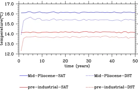
Fig. 1. Time series of global annual mean surface air
tempera-ture (◦C) and the deepest soil temperature (DST,◦C) in the pre-industrial and mid-Pliocene experiments.
file is created and tailored to the land and ocean grids (T42) at the model runtime using the above-created land surface files.
The rebuilt mid-Pliocene land cover shows greatly reduced ice volume and ice area in Greenland and Antarctic, an obvi-ous expansion of warmth/moisture-loving vegetation in the northern high latitudes and much smaller deserts in Africa, Australia and central Asia.
3.2.3 Other boundary conditions
For the greenhouse gases, the atmospheric CO2
concentra-tion increases to 405 ppmv, with the N2O concentration,
CH4concentration and ozone unchanged compared with the
pre-industrial run. The orbital parameters, solar constant and aerosol datasets are all kept as the same as in the pre-industrial run.
The two experiments have been integrated for 50 yr. A detailed experimental design is summarized in Table 1.
4 Results
Table 1. Summary of the experimental design.
Boundary conditions pre-industrial mid-Pliocene SST local modern PRISM3 SST v1.3.nc Land-sea mask local modern local modern Topography local modern topo v1.4 Ice sheets and vegetation BAS Observ BIOME biome veg v1.2 Greenhouse gases CO2=280 ppm, N2O=270 ppb,
CH4=760 ppb, CFCs=0,
O3=local modern
CO2=405 ppm, N2O=270 ppb,
CH4=760 ppb, CFCs=0,
O3=local modern
Solar constant 1365 W m−2 1365 W m−2 Aerosols local modern local modern Orbital Parameters ecc=0.016724, obl=23.446◦,
peri – 180◦=102.04◦
ecc=0.016724, obl=23.446◦, peri – 180◦=102.04◦
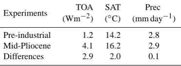
Table 2. Global annual mean of net energy at the top of atmosphere
(TOA), surface air temperature (SAT) and precipitation rate (Prec) for the pre-industrial, mid-Pliocene, and the differences between mid-Pliocene and pre-industrial.
Experiments TOA SAT Prec (Wm−2) (◦C) (mm day−1) Pre-industrial 1.2 14.2 2.8 Mid-Pliocene 4.1 16.2 2.9 Differences 2.9 2.0 0.1
4.1 Surface air temperature
For the zonal mean SAT, the CAM3.1 model simulates a dis-tinct pattern of mid to high latitude warming over oceans and continents in the mid-Pliocene (Fig. 2). The maximum warming in the zonal mean SAT is located in the high lat-itudes, where the SAT increases by approximately 10◦C (at approximately 80◦N) and 8◦C (at approximately 70◦S). However, the SAT remains nearly unchanged in the low lat-itudes. The equator-to-pole SAT gradient, defined as the SAT differences between 0–30◦N(S) and 60◦–90◦N(S), de-creases by 7.3◦C and 4.1◦C in the Northern Hemisphere and Southern Hemisphere, respectively.
The strong high latitude warming can also be observed in the spatial distribution of SAT anomalies between the mid-Pliocene and pre-industrial experiments (Fig. 3). Between 40◦N and 90◦N, the annual mean SAT is approximately 2– 16◦C higher in the mid-Pliocene than in pre-industrial. The greatest warming appears in Greenland and the sub-polar North Atlantic, with a rise of 8◦∼16◦C. Between 40◦S and 40◦N, the SAT increases by 0–2◦C in most regions. Be-tween 40◦S and 80◦S, the SAT rises by approximately 4– 18◦C. The greatest warming compared with pre-industrial
occurs in the margins of the East Antarctic and West Antarc-tic, where the SAT is 8–18◦C and 6–12◦C higher, respec-tively. The great warming over Greenland and Antarctic is attributed to the combined effects of reduced surface albdo and lower topography in the mid-Pliocene.
However, cooling is still apparent in some local regions in the mid-Pliocene. The SAT decreases by 0–2◦C over the East African rift zone and the western tropical Pacific. The SAT remains nearly unchanged or exhibits slight cooling at 80◦–90◦S in the East Antarctic.
During boreal winter (Fig. 3), the globally averaged SAT compared with the pre-industrial rises on average by 2.0◦C. The extreme warming over the high latitudes of the North-ern Hemisphere becomes stronger in comparison with the changes in annual mean SAT, with a maximum warming of ∼20◦C over the sub-polar North Atlantic. The warming ar-eas also expand. In low latitudes, the magnitude of warming is unchanged. In contrast, the magnitude of warming in the Southern Hemisphere between 60◦S and 90◦S decreases by about 2–3◦C.
Fig. 2. Zonal mean surface air temperature (◦C) in the pre-industrial experiment (a), the mid-Pliocene experiment (b) and the anomalies between the mid-Pliocene and pre-industrial (c).
4.2 Precipitation
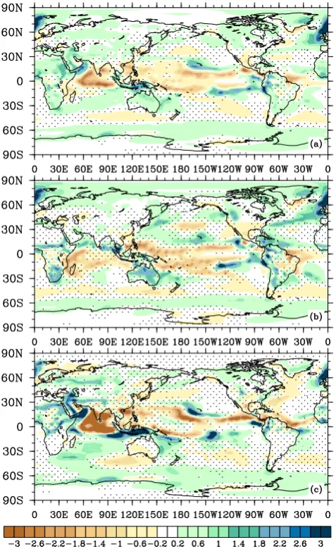
Compared with pre-industrial, annual mean precipitation is enhanced over the continents in the mid-Pliocene, with great increases (0.8–1.6 mm day−1) over South Greenland, Africa, the Middle-East region, Australia and the west coast of South America (Fig. 4). Over the oceans, the precipitation is enhanced (∼3.0 mm day−1) over the sub-polar North At-lantic and the cold tongue in the eastern tropical Pacific. In contrast, the precipitation decreases significantly by 0.8– 3 mm day−1 and 0.2–2.6 mm day−1 over the North Indian
Ocean and the InterTropical Convergence Zone (ITCZ), re-spectively. Decreased precipitation is also simulated in the tropical Atlantic. Generally, the changes in precipitation are greater at low latitudes than at high latitudes.
During boreal winter (Fig. 4), the spatial distribution and magnitude of precipitation anomalies are nearly unchanged compared with the anomalies of the annual mean precip-itation. During boreal summer (Fig. 4), the precipitation
Fig. 3. Surface air temperature anomaly (◦C) between the mid-Pliocene experiment and the pre-industrial experiment for the an-nual period (a), winter (b) and summer (c) seasons. Areas with a confidence level less than 95 % are dotted.
decreases much more (>3.2 mm day−1) over the North In-dian Ocean and the ITCZ compared with the changes in an-nual mean precipitation. In contrast, the precipitation is en-hanced over North Africa, the Middle-East region, Indonesia, and the adjacent oceans. The area of enhanced precipitation over the sub-polar Atlantic becomes smaller. However, the global mean summer precipitation remains unchanged com-pared with the pre-industrial.
5 Discussion
Fig. 4. Same as in Fig. 3 but for the precipitation anomaly (mm day−1).
latitudes. Thus, the equator-to-pole temperature gradient is reduced.
Due to the reduced temperature gradient, the Hadley cir-culation slows down in the mid-Pliocene compared with the pre-industrial circulation. Both the ascending branches of the Hadley cell near 10◦S–15◦N and the descending branches at approximately 15◦N–25◦N and 10◦S–20◦S are weakened (Fig. 5). The weakened descending branches of the Hadley cell enhance precipitation in the subtropics. The weakened ascending branches of the Hadley cell (approximately 10◦S– 15◦N) lead to weakened deep convection over ITCZ, which in turn causes decreased precipitation over ITCZ. In addition, the slow-down of the Hadley cell leads to weakened surface winds, namely trade winds, in the tropics. However, it should be noted that the sinking motion at the poleward edge of the Hadley cell (approximately 30◦N and 30◦S) is strengthened (Fig. 5), which may indicate the poleward expansion of the Hadley cell.
Fig. 5. Mass stream function (×109kg s−1)of the annually aver-aged zonal mean meridional circulation in the pre-industrial (a), the mid-Pliocene (b) and the differences between the mid-Pliocene and pre-industrial (c). Areas with a confidence level less than 95 % are dotted.
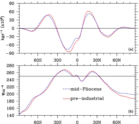
Fig. 6. (a): latitudinal cross-section of the mass stream function
at 500 hPa in the pre-industrial and mid-Pliocene. (b): zonal mean outgoing longwave radiation in the pre-industrial and mid-Pliocene.
descending branches of the Hadley cell in the mid-Pliocene expand poleward by 0.4◦and 1.0◦in the northern and south-ern hemispheres, respectively, while expand poleward by 0.6◦and 0.2◦based on the simulated outgoing longwave ra-diation (Fig. 6).
The poleward expansion of the Hadley cell is potentially important for understanding future climate under global warming (Seidel et al., 2008; Johanson and Fu, 2009). As the Hadley cell has widened by about 2◦–5◦since 1979 based on recent observations (Johanson and Fu, 2009), the poleward expansion of the Hadley cell in the mid-Pliocene is not sig-nificant. However, it should be noted that the simulation for the Hadley circulation here is mainly controlled by the pre-scribed PRISM3D SST fields. Due to the uncertainties in the reconstruction of the PRISM3D SST, it remains a task to compare our simulation with other coupled simulations.
6 Summary
In this study, using AGCM CAM3.1, we simulate the mid-Pliocene climate with the prescribed PRISM3D boundary conditions. Our simulations illustrate that the global an-nual mean SAT in the mid-Pliocene is approximately 2.0◦C higher than the pre-industrial value. The warming is stronger in the mid-high latitudes than in the low latitudes, which leads to a reduced equator-to-pole SAT gradient. The annual mean precipitation increases by 3.6 % of the pre-industrial value. However, the changes in precipitation are much greater at low latitudes than at high latitudes. Moreover, the Hadley cell expands poleward by less than 1◦ in the mid-Pliocene compared to pre-industrial.
Acknowledgements. The authors would like to thank the PRISM
workgroup for providing the mid-Pliocene boundary conditions and the CESM paleoclimate workgroup for providing the tools which were used to create boundary conditions for CAM3.1. The comments of the Topical editor, Ren´e Redler, and the reviewers, H. Dowsett and M. Krapp, helped considerably to improve the clarity of the manuscript. This work was supported by the National Basic Research Program of China (2009CB421406), the Knowledge Innovation Program of the Chinese Academy of Sciences (KZCX2-YW-Q1-02), and the National Natural Science Foundation of China (4090205 and 40975050).
Edited by: R. Redler
References
Bonan, G. B.: Land surface model (LSM version 1.0) for ecologi-cal, hydrologiecologi-cal, and atmospheric studies: Technical description and users guide, NCAR Technical Note NCAR/TN-417+STR, National Center for Atmospheric Research, Boulder, Colorado, 150 pp., 1996.
Bonan, G. B., Levis, S., Kergoat, L., and Oleson, K. W.: Land-scapes as patches of plant functional types: An integrating con-cept for climate and ecosystem models, Global Biogeochem. Cy., 16, 1021, doi:10.1029/2000GB001360, 2002a.
Bonan, G. B., Oleson, K. W., Vertenstein, M., Levis, S., Zeng, X., Dai, Y., Dickinson, R. E., and Yang, Z. L.: The land surface climatology of the community land model coupled to the NCAR community climate model, J. Climate, 15, 3123–3149, 2002b. Briegleb, B. P., Bitz, C. M., Hunke, E. C., Lipscomb, W. H.,
Hol-land, M. M., Schramm, J. L., and Moritz, R. E.: Scientific de-scription of the sea ice component in the community climate sys-tem model, version Three, Technical Note NCAR/TN-463+STR, National Center for Atmospheric Research, Boulder, Colorado, 78 pp., 2004.
Caballero, R. and Huber, M.: Spontaneous transition to superrota-tion in warm climates simulated by CAM3, Geophys. Res. Lett., 37, L11701, doi:10.1029/2010GL043468, 2010.
Chandler, M., Rind, D., and Thompson, R.: Joint investigations of the middle Pliocene climate II: GISS GCM Northern Hemisphere results, Global Planet. Change, 9, 197–219, 1994.
Collins, W. D., Rasch, P. J., Boville, B. A., Hack, J. J., McCaa, J. R., Williamson, D. L., Kiehl, J. T., Briegleb, B., Bitz, C., and Lin, S.: Description of the NCAR community atmosphere model (CAM 3.0), NCAR Technical Note NCAR/TN-464+STR, National Center for Atmospheric Research, Boulder, Colorado, 226 pp., 2004.
Collins, W. D., Rasch, P. J., Boville, B. A., Hack, J. J., McCaa, J. R., Williamson, D. L., Briegleb, B. P., Bitz, C. M., Lin, S. J., and Zhang, M.: The formulation and atmospheric simulation of the Community Atmosphere Model version 3 (CAM3), J. Climate, 19, 2144–2161, 2006.
Diffenbaugh, N. S. and Ashfaq, M.: Response of California Current forcing to mid-Holocene insolation and sea surface temperatures, Paleoceanography, 22, PA3101, doi:10.1029/2006PA001382, 2007.
Dowsett, H. J.: The PRISM palaeoclimate reconstruction and Pliocene sea-surface temperature, in: Deep time perspectives on climate change: Marrying the signal from computer models and biological proxies, edited by: Williams, M., Haywood, A. M., Gregory, F. J., and Schmidt, D. N., the Micropalaeontological Society, Special Publications, the Geological Society, London, 459–480, 2007.
Dowsett, H. J. and Poore, R. Z.: Pliocene sea surface temperatures of the North Atlantic Ocean at 3.0 Ma., Quaternary Sci. Rev., 10, 189–204, 1991.
Dowsett, H. J., Cronin, T. M., Poore, R. Z., Thompson, R. S., What-ley, R. C., and Wood, A. M.: Micropaleontological evidence for increased meridional heat transport in the North Atlantic Ocean during the Pliocene, Science, 258, 1133–1135, 1992.
Dowsett, H. J., Thompson, R., Barron, J., Cronin, T., Fleming, F., Ishman, S., Poore, R.,Willard, D., and Holtz, T.: Joint investiga-tions of the middle Pliocene climate I: PRISM paleoenvironmen-tal reconstructions, Global Planet. Change, 9, 169–195, 1994. Dowsett, H. J., Barron, J., and Poore, R.: Middle Pliocene sea
sur-face temperatures: a global reconstruction, Mar. Micropaleon-tol., 27, 13–25, 1996.
Dowsett, H. J., Barron, J. A., Poore, R. Z., Thompson, R. S., Cronin, T. M., Ishman, S. E., and Willard, D. A.: Middle Pliocene pale-oenvironmental reconstruction: PRISM2, US Geol. Surv., Open File Rep., 99–535, 1999.
Dowsett, H. J., Robinson, M. M., and Foley, K. M.: Pliocene three-dimensional global ocean temperature reconstruction, Clim. Past, 5, 769–783, doi:10.5194/cp-5-769-2009, 2009.
Dowsett, H. J., Robinson, M. M., Haywood, A. M., Salzmann, U., Hill, D., Sohl, L., Chandler, M., Williams, M., Foley, K., and Stoll, D.: The PRISM3D paleoenvironmental reconstruction, Stratigraphy, 7, 123–139, 2010.
Edwards, M.: Global Gridded Elevation and Bathymetry, Global Ecosystems Database, Version 1.0 (on CD-ROM), Documenta-tion Manual, Disc-A: NaDocumenta-tional Geophysical Data Center, Key to Geophysical Records Documentation No. 26, Incorporated in: Global Change Database, Volume 1, edited by: Kineman, J. J. and Ohrenschall, M. A., Boulder, CO, National Oceanic and At-mospheric Administration, 14-1 to A14-4, 1992.
Global Soil Data Task: Global Soil Data Products CD-ROM (IGBP-DIS), CD-ROM, International Geosphere-Biosphere Pro-gramme, Data and Information System, Potsdam, Germany, 2000.
Haywood, A. M. and Valdes, P. J.: Modelling Pliocene warmth: contribution of atmosphere, oceans and cryosphere, Earth Planet. Sci. Lett., 218, 363–377, 2004.
Haywood, A. M., Valdes, P. J., and Sellwood, B. W.: Global scale palaeoclimate reconstruction of the middle Pliocene climate us-ing the UKMO GCM: initial results, Global Planet. Change, 25, 239–256, 2000.
Haywood, A. M., Dowsett, H. J., Otto-Bliesner, B., Chandler, M. A., Dolan, A. M., Hill, D. J., Lunt, D. J., Robinson, M. M., Rosenbloom, N., Salzmann, U., and Sohl, L. E.: Pliocene Model Intercomparison Project (PlioMIP): experimental design and boundary conditions (Experiment 1), Geosci. Model Dev., 3, 227–242, doi:10.5194/gmd-3-227-2010, 2010.
Hill, D. J., Haywood, A. M., Hindmarsh, R. C. A., and Valdes, P. J.: Characterising ice sheets during the mid Pliocene: evidence from data and models, in: Deep time perspectives on climate change:
Marrying the signal from computer models and biological prox-ies, edited by: Williams, M., Haywood, A. M., Gregory, F. J., and Schmidt, D. N., the Micropalaeontological Society, Special Publications, the Geological Society, London, 517–538, 2007. Huber, M. and Caballero, R.: The early Eocene equable climate
problem revisited, Clim. Past, 7, 603–633, doi:10.5194/cp-7-603-2011, 2011.
Jansen, E., Overpeck, J., Briffa, K., Duplessy, J., Joos, F., Masson-Delmotte, V., Olago, D., Otto-Bliesner, B., Peltier, and W., Rahmstorf, S.: Palaeoclimate, in: Climate change 2007: The Physical Science Basis, Contribution of Working Group I to the Fourth Assessment Report of the Intergovernmental Panel on Climate Change, edited by: Solomon, S., Qin, D., Manning, M., Chen, Z., Marquis, M., Averyt, K. B., Tignor, M., and Miller, H. L., Cambridge University Press, Cambridge, United Kingdom and New York, NY, USA, 440–442, 2007.
Jiang, D., Wang, H., Ding, Z., Lang, X., and Drange, H.: Mod-eling the middle Pliocene climate with a global atmospheric general circulation model, J. Geophys. Res., 110, D14107, doi:10.1029/2004JD005639, 2005.
Jochum, M., Fox-Kemper, B., Molnar, P., and Shields, C.: Differ-ences in the Indonesian seaway in a coupled climate model and their relevance to Pliocene climate and El Ni˜no, Paleoceanogra-phy, 24, PA1212, doi:10.1029/2008PA001678, 2009.
Johanson, C. M. and Fu Q.: Hadley cell widening: Model simula-tion versus observasimula-tions, J. Climate, 22, 2713–2725, 2009. Liang, X. Z., Wang, W. C., and Boyle, J. S.: Atmospheric ozone
climatology for use in general circulation models, Tech. Rep. 43, PCMDI, 25 pp., 1997.
Lu, J., Vecchi G. A., and Reichler T.: Expansion of the Hadley cell under global warming, Geophys. Res. Lett., 34, L06805, doi:10.1029/2006GL028443, 2007.
Lunt, D. J., Haywood, A. M., Schmidt, G. A., Salzmann, U., Valdes, P. J., and Dowsett, H. J.: Earth system sensitivity inferred from Pliocene modelling and data, Nat. Geosci., 3, 60–64, 2010. Matthews, E.: Prescription of land-surface boundary conditions in
GISS GCM II: A simple method based on high-resolution vege-tation data bases, NASA Report No. TM 86096, 20 pp., 1985. Rayner, N. A., Parker, D. E., Horton, E. B., Folland, C. K.,
Alexan-der, L. V., Powell, D. P., Kent, E. C., and Kaplan, A.: Global analyses of sea surface temperature, sea ice, and night marine air temperature since the late nineteenth century, J. Geophys. Res., 108, 4407, doi:10.1029/2002JD002670, 2003.
Reynolds, R. W. and Smith, T. M.: A high-resolution global sea sur-face temperature climatology, J. Climate, 8, 1571–1583, 1995. Reynolds, R. W., Rayner, N. A, Smith, T. M., Stokes, D. C., and
Wang, W.: An improved in situ and satellite SST analysis for climate, J. Climate, 15, 1609–1625, 2002.
Robinson, M. M., Dowsett, H. J., Dwyer, G. S., and Lawrence, K. T.: Reevaluation of mid-Pliocene North At-lantic sea surface temperatures, Paleoceanography, 23, PA3213, doi:10.1029/2008PA001608, 2008.
Salzmann, U., Haywood, A. M., Lunt, D. J., Valdes, P. J., and Hill, D. J.: A new global biome reconstruction and data-model com-parison for the middle Pliocene, Global Eco. Biogeogr., 17, 432– 447, 2008.
Sloan, L. C., Crowley, T. J., and Pollard, D.: Modeling of middle Pliocene climate with the NCAR GENESIS general circulation model, Mar. Micropaleontol., 27, 51–61, 1996.
Sohl, L. E., Chandler, M. A., Schmunk, R. B., Mankoff, Ken, Jonas, J. A., Foley, K. M., and Dowsett, H. J.: PRISM3/GISS topo-graphic reconstruction: US Geol. Surv. Data Series 419, 6 pp., 2009.
Wei, T., Wang, L., Dong, W., Dong, M., and Zhang J.: A compar-ison of East Asian summer monsoon simulations from CAM3.1 with three dynamic cores, Thero. Appl. Climatol., 106, 295–306, 2011.
Yan, Q., Zhang, Z., Wang, H., Jiang, D., and Zheng, W.: Simulation of sea surface temperature changes in the middle Pliocene warm period and comparison with reconstructions, Chinese Sci. Bull., 56, 890–899, 2011.