https://doi.org/10.5194/gmd-10-3519-2017 © Author(s) 2017. This work is distributed under the Creative Commons Attribution 3.0 License.
Reverse engineering model structures for soil and ecosystem
respiration: the potential of gene expression programming
Iulia Ilie1, Peter Dittrich2,3, Nuno Carvalhais1,4, Martin Jung1, Andreas Heinemeyer5, Mirco Migliavacca1, James I. L. Morison8, Sebastian Sippel1, Jens-Arne Subke6, Matthew Wilkinson8, and Miguel D. Mahecha1,3,7
1Max Planck Institute for Biogeochemistry, Department Biogeochemical Integration, Hans-Knoell-Str. 10,
07745 Jena, Germany
2Bio Systems Analysis Group, Institute of Computer Science, Jena Centre for Bioinformatics and
Friedrich Schiller University, 07745 Jena, Germany
3Michael Stifel Center Jena for Data-Driven and Simulation Science, 07745 Jena, Germany
4CENSE, Departamento de Ciéncias e Engenharia do Ambiente, Faculdade de Ciéncias e Tecnologia,
Universidade NOVA de Lisboa, Caparica, Portugal
5Department of Environment, Stockholm Environment Institute, University of York, York, YO105NG, UK 6Biological and Environmental Sciences, School of Natural Sciences, University of Stirling, Stirling, UK 7German Centre for Integrative Biodiversity Research (iDiv), Deutscher Platz 5e, 04103 Leipzig, Germany 8Forest Research, Alice Holt Lodge, Farnham, Surrey, GU10 4LH, UK
Correspondence to:Iulia Ilie ([email protected]) and Miguel D. Mahecha ([email protected]) Received: 29 September 2016 – Discussion started: 7 November 2016
Revised: 31 July 2017 – Accepted: 21 August 2017 – Published: 25 September 2017
Abstract. Accurate model representation of land– atmosphere carbon fluxes is essential for climate projections. However, the exact responses of carbon cycle processes to climatic drivers often remain uncertain. Presently, knowledge derived from experiments, complemented by a steadily evolving body of mechanistic theory, provides the main basis for developing such models. The strongly increasing availability of measurements may facilitate new ways of identifying suitable model structures using machine learning. Here, we explore the potential of gene expression programming (GEP) to derive relevant model formulations based solely on the signals present in data by automatically applying various mathematical transformations to potential predictors and repeatedly evolving the resulting model struc-tures. In contrast to most other machine learning regression techniques, the GEP approach generates “readable” models that allow for prediction and possibly for interpretation. Our study is based on two cases: artificially generated data and real observations. Simulations based on artificial data show that GEP is successful in identifying prescribed functions, with the prediction capacity of the models comparable to four state-of-the-art machine learning methods (random
forests, support vector machines, artificial neural networks, and kernel ridge regressions). Based on real observations we explore the responses of the different components of terres-trial respiration at an oak forest in south-eastern England. We find that the GEP-retrieved models are often better in prediction than some established respiration models. Based on their structures, we find previously unconsidered expo-nential dependencies of respiration on seasonal ecosystem carbon assimilation and water dynamics. We noticed that the GEP models are only partly portable across respiration components, the identification of a “general” terrestrial respiration model possibly prevented by equifinality issues. Overall, GEP is a promising tool for uncovering new model structures for terrestrial ecology in the data-rich era, complementing more traditional modelling approaches.
1 Introduction
quantitative description of the terrestrial carbon cycle (Bo-nan, 2008; Heimann and Reichstein, 2008; Luo et al., 2015). However, the description of the mechanisms underlying the total terrestrial efflux of CO2 (S. Peng et al., 2014),
of-ten referred to as “terrestrial ecosystem respiration” (Reco),
varies across the scientific literature and existing global mod-els. This is partly because Reco does not originate from a
single process but is the sum of fluxes from different au-totrophic and heterotrophic respiration processes that oper-ate across different temporal and spatial scales and compart-ments (e.g. soil depths). Hence, it is experimentally very dif-ficult to disentangle the main abiotic and biotic factors driv-ing respiratory processes at the ecosystem level (Trumbore, 2006) and to derive suitable models for the individual res-piration processes. In the rest of the paper we use the term “model” as an equivalent of “response functions”, i.e. some analytic description of how environmental drivers influence ecosystem fluxes.
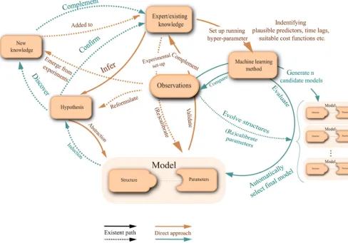
Traditionally, respiration models have been based on some theoretical considerations, but largely remain empirical in nature (e.g. Reichstein and Beer, 2008; Gilmanov et al., 2010; Hoffmann et al., 2015). Conventional model building (Fig. 1) is primarily hypothesis driven and capitalizes both on some understanding of the system and reported scaled ex-periments (Migliavacca et al., 2012; Richardson et al., 2008). Gupta et al. (2012) describe this common paradigm of model development as a four-step approach involving observational, conceptual, mathematical and computational phases (see also e.g. Bennett et al., 2010; Williams et al., 2009). During the observational phase, the system under scrutiny is monitored and observations are assembled, ideally representing process responses to hypothesized driving variables. Based on these observations, a conceptual model is proposed, which subse-quently guides the formulations of mathematical represen-tations of the system states and dependencies. The mathe-matical description then provides the basis for computational models that are used for simulations (Jakeman et al., 2006). Model–data integration may additionally lead to iterative structural revisions or parameter optimizations (Williams et al., 2009). This conventional approach to model devel-opment is also characteristic of different kinds of ecological model building, including the development of biogeochemi-cal models (Williams et al., 2009).
We explore the possibility of reverse engineering offering an automated alternative to model development for predict-ing terrestrial carbon fluxes (Fig. 1). In reverse engineerpredict-ing, the work flow is fundamentally different (Bongard and Lip-son, 2007), comprising a database set-up phase, a computa-tional phase, a mathematical phase and a conceptual phase (Gupta et al., 2012). The rationale behind reordering the key phases is firstly to minimize the human influence and perception biases that might shape the formulation of new hypotheses, and secondly to increase the chance of novel model structures automatically emerging from the available data and that would not be so obvious from a direct analysis.
Reverse engineering aims at identifying some mathematical representation of a system that is to a large degree indepen-dent of a priori conceptualizations: in the current case, the respiratory response of terrestrial ecosystems to environmen-tal drivers. Reverse engineering leaves the model construc-tion up to an algorithm and is therefore a way to empirically learn from observations with minimal user input.
Of course, expert knowledge still has a large influence on the modelling process, as only a certain set of variables can be measured and an even smaller subset is indeed available for model development, which includes the restriction to a certain plausible number of time lags, and hence full ob-jectivity of automatic model development cannot be truly achieved. Furthermore, expert knowledge comes into play when the algorithm is set for running, by tuning the set of parameters according to the problem needed to be solved and as well during the observation collection and during the final decision on whether the solution returned by the algorithm actually makes sense at all and whether it can be used further. Nevertheless, we believe that by shifting the moment when the analyst makes the decision regarding the selected model, a larger degree of objectivity in modelling is achieved.
Reverse engineering is close to machine learning based regression techniques, where various candidate model for-mulations and specifications are explored in order to mini-mize the prediction error. The fundamental difference from typical model building is that reverse engineering typically provides a symbolic regression, that is, the resulting struc-tures are ideally directly readable as mathematical functions (i.e. response functions) and can be interpreted. The read-able character of the returned solutions allows us to consider the applicability of the derived structures in other system do-mains (Ashworth et al., 2012).
Here, we focus on the gene expression programming (GEP, Ferreira, 2001) reverse engineering approach. GEP is an evolutionary algorithm that constructs mathematical re-sponse functions. In its essence, GEP basically converges to a solution after rejecting a large number of potential regres-sion models over a certain number of evolutionary steps. Due to its structural design, GEP can be applied in a wide range of empirical modelling problems (Y. Peng et al., 2014; Khat-ibi et al., 2013; Traore and Guven, 2013), including (soil) hydrology (Fernando et al., 2009; Hashmi and Shamseldin, 2014). To the best of our knowledge the potential of GEP has not yet been explored for modelling biogeochemical fluxes in terrestrial ecosystems.
We seek to understand as well whether automating model development can provide new insights into understanding the dynamics of terrestrial respiration processes. We base our study on data from a long-term monitoring experiment of Reco components, i.e. above-ground respiration, root
Figure 1.Direct approach and reverse engineering in model development for describing dynamical systems. Existing and possible steps needed in the process of building a model. For the direct approach, the process starts with the building of a hypothesis from existing knowledge. The hypothesis is then the subject of abstraction and is summarized in a mathematical model that has two components: the structure and the parameters. The mathematical model can be translated into a computational form that will generate predictions. Depending on how well the predicted values manage to recreate the available observations, the model’s parameters are calibrated or, if the general trends are missed, there might be a need for structural reformulation. On the other hand, in the reverse engineering approach, a machine learning method is used to generate a set of candidate models that are then compared with the available observations and which according to the prediction capacity may have to go through structural changes by automatic evolution or through a final parameter adaptation. From the set of evolved models, the best model in terms of prediction capacity is chosen and its structure will be the basis for hypothesis building, as an expert would try to explain why a specific structure was automatically evolved and whether the structure of the model can be explained from the studied system-intrinsic processes. If that is the case, and the structure has not emerged randomly, the conclusions can be compared with the existing knowledge which can be reconfirmed, or new aspects of the studied system might be brought to light.
The fundamental question addressed in this paper is whether regression models can be constructed more objec-tively by leaving the task of proposing a final regression model to an algorithm rather than directly to an analyst. The need for human intuition during the actual process of con-structing a regression model becomes reduced, and the input of expert knowledge shifts towards identifying input vari-ables, parameters, a suitable cost function and model plau-sibility.
With the current study we investigate as well whether auto-matically derived model structures differ substantially from models conventionally used in the study ofRecoand its
com-ponents or whether they are consistent with established the-ory. The separation ofRecointo its components also allowed
us to test the portability of individual model structures across different respiration components. In this sense, we investi-gate whether a generic “respiration” response can be derived or whether specific formulations for a range of respiration components are required.
Study structure
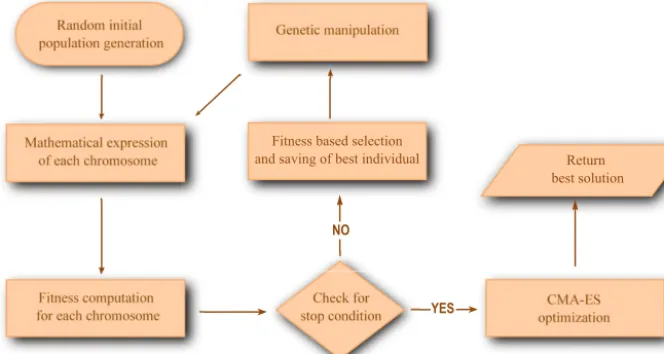
us-Figure 2.The work flow used in solving symbolic regression problems with GEP. The process of evolving an optimal solution from ob-servations starts with randomly generating a set number of evolution individuals called chromosomes. The chromosomes are composed of genes that are sets of strings encoding expression trees that can be translated into mathematical expressions in the subsequent step. Following the mathematical expression comes the evaluation of each emerging individual (model) against the target variable values and for each one a fitness value is assigned. If the stopping criterion has not been reached (e.g. best fitness possible, highest number of generations allowed, con-vergence) the best individual in terms of fitness is saved and the remaining set of chromosomes are selected for genetic manipulation. When the stop criterion is reached, the parameters of the best chromosome is calibrated against the training data with an optimization approach, the CMA-ES, and the best solution is returned.
ing an artificial experiment under varying degrees of noise contamination designed to resembleReco. Second, we apply
GEP to model the various respiration observations provided by Heinemeyer et al. (2012).
The observational record provided by Heinemeyer et al. (2012) is exceptional, because measurements of soil or ecosystem respiration that are typically only integrated are here continuously and regularly measured, and the compo-nents measured offer a perfect test case for the GEP method-ology.
For both the artificial experiment and real-world observa-tions, we systematically confront the prediction error of GEP with other state-of-the-art machine learning regression ap-proaches. In addition, we adjust the modelling approach such that the objective function (or fitness function) not only ac-counts for absolute or relative error, but also reduces struc-ture in the residuals. The discussion focuses on the compar-ison of the various GEP-derived models, their equifinality, and performance compared to widely used literature models.
2 Method
We rely on the GEP method (Ferreira, 2001) which automat-ically constructs model structures based on a set of given ob-servations. As the models we want to obtain are mathemati-cal structures, their construction can be achieved by solving a symbolic regression (Kotanchek et al., 2013) type of prob-lem. That is, we are not only interested in determining an op-timal set of parameters for a known regression, but here, we
want to discover the symbolic form of the regression itself by identifying the most important predictors and their functional transformations. The general GEP approach in solving sym-bolic regressions is presented in the following section and is illustrated in Fig. 2.
2.1 Gene expression programming, GEP
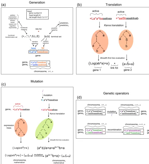
The process of finding the most suitable model structure based on the signal present in data in GEP starts with an initial generation of n possible model structures (Fig. 3a). These can be called evolution individuals and in GEP they are known as “chromosomes”. The chromosomes are com-posed of a fixed number of “genes” that are connected by a binary mathematical operator. Each gene is encoded in a string with a fixed length that contains specific characters that map to either a set of possible predictors, e.g.A= {a, b} →Am= {x1, x2}, or a set of their possible functional
transformations, e.g. F= {+, −, L, E} →Fm= {addition,
substraction, logarithm, exponential}(see Fig. 3a).
solu-(a)
(b)
(d)
(c)
tion, the user can define a new function and introduce it in the set of input functions.
All genes are made up of a “gene head”, containing a combination of characters mapping to both predictors and functional transformations, and a “gene tail”, with charac-ters that map only to predictors. The gene length is given by gl=hl+tl, wheretl=(fmax−1)×hl+1, with gl as gene
length,hl head length,tl tail length andfmaxthe maximum
parity of a functional transformation.
As in biology evolution, regardless of the actual length, the GEP genes have active sections of variable length called “open reading frames” (ORFs) that can encode various pression trees which can be evaluated into mathematical ex-pressions (Ferreira, 2006). The lengths of the ORFs are de-termined only after the encoded expression trees are trans-lated using an internal reading language (see Fig. 3b). Fer-reira (2001) argues that the power of GEP lies in its use of fixed length linear strings for representing trees (ET) of var-ied shapes and sizes that simplify the evolutionary process and help reach a final solution faster.
The total number of chromosomes generated over each evolution step make up the GEP population. The evolution steps are also known as “generations”. The maximum num-ber of generations allowed to run until reaching a solution is often used as a stopping criterion.
One of the crucial components of model development within an evolutionary algorithm is the selection process. In GEP, the chromosomes can be translated into mathematical expressions that can be evaluated, and a distance between the current structure based predictions and the original tar-get is computed. The measures are known as “fitness values” and are assigned to all the chromosomes in the population at each generation by means of a predefined fitness function. The evolution of the final solution with GEP is done based on optimizing the fitness function values after each generation, usually by minimizing prediction error, but more complex criteria can be taken into account as well.
Once all the fitness values have been computed and as-signed, the chromosomes in a generation are sorted from best to worst fit.
If no stop criteria have been met, preparations for the re-production of new chromosomes for the next generation are made. The chromosome with the best fitness value is repro-duced unchanged in the first position of the new generation. To fill the remainingn−1 positions, chromosomes are se-lected from the entire population for the new generation with a tournament proceduren−1 times.
In tournament selection, two chromosomes are randomly selected from the entire population and the individual with the better fitness value goes through.
To ensure that novel material is introduced in the pool of possible model structures,n−1 newly selected chromo-somes are subject to genetic operators, such as mutation, recombination, transposition and inversion as presented in
Fig. 3d, which can fully change the encoded mathematical expressions (see Fig. 3c).
Once the population of chromosomes is ready for the new generation, the evolution procedure is repeated until a stop criterion is reached, such as best fitness achieved, maximum number of unimproved generations reached, or time limit.
The hyper-parameter needed for a GEP run, i.e. the set of all parameters that need to be fixed before a GEP run is performed, has either components with recommended de-fault values, especially for the genetic operator rates consid-ered when applying the available genetic operators (Ferreira, 2006), or has components for which the values have been established empirically after experience in working with the GEP approach. The latter typically depend on the require-ments of the problem to solve.
Such is the case for setting the length of the gene head or the number of genes in a chromosome that can be lower if the interest is in obtaining more compact solutions, with larger values possibly leading to a fast expansion of solution length which can easily overfit the initial target. When the lengths of the chromosomes are kept too low, the structures in the pop-ulation can converge too soon to a unique solution that might lack the ability to capture meaningful signals present in the training data, due to low diversity of the encoded expression trees.
Another important component of the hyper-parameter to fix is the mutation rate, which is one of the genetic variation operators. When the mutation rate is too large, it can become disruptive and lead to loss of information acquired along the previous evolutionary time steps, reducing the general con-vergence of the GEP run. Conversely, if the rate is too low, relevant structures may not be constructed in the given time limit.
The current implementation of the GEP approach does not contain an explicit population diversity management compo-nent which could increase the confidence that a certain solu-tion did not just appear by chance but was actually selected over a larger pool of possible model structure types. In or-der to reduce stochastic bias and avoid getting stuck in local optima that would produce overfitted results, we chose the practical approach of multi-start (multiple runs with the same settings) as proposed by Ferreira (2006).
2.2 Fitness measure
In our study, the fitness measure is reported in terms of the Nash–Sutcliffe modelling efficiency (MEF) coefficient (Nash and Sutcliffe, 1970; Bennett et al., 2010) which is of-ten used in the context of quantifying the performance of ter-restrial biosphere models (Mitchell et al., 2009; Migliavacca et al., 2015). The MEF is computed as
MEF=1−
n P
i=1
(oi−pi)2 n
P
i=1
(oi−o)2
(1)
whereoi is the observed value at stepi,pi is the predicted value at step iandois the mean of observed values. MEF values range between−∞and 1, where an MEF value of 1 corresponds to the case where the predicted and observed values are identical. A negative MEF value means that the predictions are worse than the mean of the observations in recreating the observed signal. MEF=0 indicates that the model predictions are as good as a prediction byo.
During the GEP learning process, however, we use the (1−MEF) measure as we want to minimize the fitness func-tion values.
Although the MEF metric offers a straightforward inter-pretation, it does not take the number of parameters of the models into account. In real-world applications, it might be desirable to derive models with fewer parameters if those are not (much) worse in terms of prediction capacity than mod-els with a higher number of free terms. Thus, we include in our cost (fitness) function a normalized term related to the number of parameters (ratio of the current number of param-eters to the maximum number of possible paramparam-eters given the GEP run settings).
Moreover, any systematic pattern in the model residuals needs to be reduced as the latter should ideally only rep-resent uncorrelated noise. To meet this criterion, we com-plement the fitness function with a term related to the in-formation content (entropy) in the residual time series. En-tropy values would be maximized for data without structure (i.e. white noise), and lower entropy values would be ob-tained for structured data, e.g. correlated stochastic or de-terministic processes (Rosso et al., 2007). The information content in a time series is typically quantified by the Shan-non entropy (SE, ShanShan-non, 1948), i.e. a term of the form
SE(X)= −
N X
i=1 piln
pi
. (2)
Here,X= {pi;i=1, . . . ,N}denotes a probability distribu-tion with
N P
i=1
pi=1 andN possible states.
In short, the calculation of an entropy as a measure for ran-domness from a time series (e.g. Shannon’s entropy) requires
us to determine a probability distribution that underlies the time series (or dynamical system), which is usually done by a partitioning step (also called phase space reconstruction in other contexts). This is a fundamental step in the method-ology, and various methods have been used to arrive at this probability distribution, for instance frequency or histogram-based measures, procedures histogram-based on amplitude statistics, or symbolic dynamics (see e.g Kowalski et al., 2011, for an overview).
As our aim is to minimize structure in the residuals, the temporal order becomes important. In recent years, the Bandt–Pompe approach has become popular, because it di-rectly takes time sequences into account: the technique hence divides the time series into ordinal sequences (i.e. ordinal patterns, or symbolic sequences), and then computes entropy measures directly from the probability distribution of these ordinal patterns (Bandt and Pompe, 2002).
This approach has a number of advantages, namely that it is robust to noise (no sensitivity to numeric outliers) and to trends or drift in the data, it is an (almost) non-parametric method and no prior assumptions about the data are needed (the only parameter that has to be specified is the embedding dimension, i.e. window length), and it allows us to disentan-gle various possible states of the system that are then encoded in the probability distribution (see e.g. Zanin et al., 2012, for a review of the method and applications).
The single parameter that needs specification is the win-dow length. This parameter is fixed tondemb=4 throughout
the entire paper following previous work on ecosystem gross primary productivity dynamics by Sippel et al. (2016).
The final normalized form of the fitness function further used in our work is
CEM=
s
(1−MEF)2+
P
Pmax 2
+(1−SE)2, (3)
Pmax=ng×l, (4)
where CEM stands from here on for “complexity corrected efficiency in modelling”, P is the number of parameters present in a model structure,Pmaxis the maximum number
of parameters possible for each individual from a GEP run set-up,ngis the number of genes in a chromosome andlis
the length of a gene.
To assess the effect of adding the entropy component for the residuals in the CEM fitness function, we introduce as well a fitness measure containing elements regarding only the MEF and the number of parameters.
MEF+NP=
s
(1−MEF)2+
P Pmax
2
2.3 Parameter optimization
The GEP algorithm does not have a specific treatment of con-stants in the building of model formulations, but mutations can change both the model structure and constants. However, the scaling of constant values (model parameters) might be a decisive factor in adequately determining the fitness of a formulation. Without this, a model structure might be dis-carded regardless of potentially being a very powerful candi-date. Furthermore, model parameters are often very informa-tive regarding a system’s sensitivity to some modifications of the drivers. These aspects have led to the addition of a final parameter optimization step at the end of each GEP run.
In order to obtain an optimal set of parameters for the GEP-extracted model structures, an approach that would be applicable in a large set of generated search spaces was nec-essary. Here we use the covariance matrix adaptation evolu-tion strategy (CMA-ES, Hansen et al., 2003) for optimiza-tion. The CMA-ES is a stochastic optimization algorithm that seeks to minimize a fitness function by estimating and adapting a covariance matrix according to a sampling from a multivariate normal distribution (Beyer and Schwefel, 2002; Auger and Hansen, 2005). According to Hansen (2006), one of the main arguments in favour of the CMA-ES approach is that it has shown good results even in the case of ill-posed problems (Kabanikhin, 2008), which may very well be the case for some of the GEP structures that are automatically generated.
The CMA-ES version used for the final step of optimiza-tion is the Hansen Python implementaoptimiza-tion found at https: //pypi.python.org/pypi/cma.
3 Experimental design
To explore the possibility of using GEP in developing rel-evant model structures for describing the terrestrial carbon fluxes, two case studies were designed: firstly, an experiment based on artificially generated data to better understand and present the general properties and capacities of GEP. Sec-ondly, we explored the use of GEP on real measurements of various respiratory flux components monitored continuously over 2 years in an oak forest (Heinemeyer et al., 2011). 3.1 Artificial experiments
These experiments were designed to explore whether our im-plementation of the GEP method is suitable for symbolic re-gression types of problems, and how robust/vulnerable it is across various signal-to-noise ratios. We explored a set of functions with increasing levels of non-linearity to generate data points.
f (x1)=2x1+1 (6)
f (x1)=x21+3x1+5 (7)
f (x1)=ex1+1 (8)
f (x1)=e−x1−x1 (9)
f (x1)=x12−4 sin(x1) (10)
f (x1)=x13+6x21+11x1−6 (11)
f (x1, x2)=x2x1 (12)
f (x1, x2)=x2x1−3 cos(x1) (13)
f (x1, x2)=2x12+3x22 (14)
f (x1, x2, x3)=2x12+3x22+2 sin(x3) (15)
Two-thousand data points were randomly generated with x1∈[1, 20],x2∈[1, 5], andx3∈[1, 100], and all the
func-tional transformations were done based on the same ini-tial set of 2000 data points. Out of the 2000 data points, 1000 data points were used for training, while 1000 data points were reserved for validation. The GEP settings used for each of the 20 runs are given in Table 1. If a returned structure was identical to the originally prescribed function or if (1−MEF)≤10−5at validation, the retrieval of the orig-inal structure was considered to be a success. To allow the ap-proaches to do an automatic feature selection, all three vari-ables,x1,x2, andx3, were used for learning and validation
for all 10 functions in the benchmark set.
To investigate the capacity of GEP to reconstruct a simple model used in the ecology field as well, we introduced as well an artificial test for the “Q10” model that is used in the
field for simulating the response of ecosystem respiration to change in air temperature of 10◦C at a reference temperature of 15◦C. The formulation we used for the “Q10” model is
Reco=2(0.1Tair−1.5) (16)
withRecothe ecosystem respiration flux andTairthe air
tem-perature. Again, we generated 2000 data points for both pre-dictor and target and we used half for training 100 runs and half for validation. The modelling capacity of the best struc-ture in terms of fitness value at validation is reported.
In order to investigate the response of the GEP approach to noise-contaminated data, we simulated Gaussian noise that scales with signal amplitude as often observed in the case of terrestrial ecosystem (Lasslop et al., 2012) and soil respi-ration (Lavoie et al., 2015) fluxes. The signal-to-noise ratio (SNR, measured as ratios of standard deviations) was varied between 10 and 1 in six steps.
For each of these functions and SNR levels, we sampled 100 validation data points 10 times; 20 GEP runs were per-formed on the 1000 training data points and the GEP model structure with the highest mean MEF value over the 10 vali-dation sets was chosen.
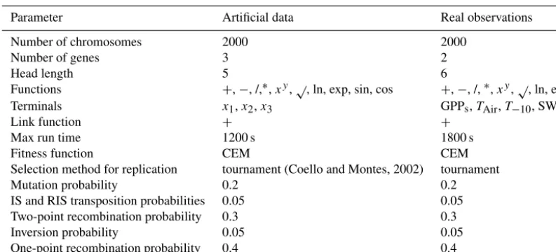
Table 1.GEP settings.
Parameter Artificial data Real observations
Number of chromosomes 2000 2000
Number of genes 3 2
Head length 5 6
Functions +,−, /,∗,xy,√, ln, exp, sin, cos +,−, /,∗,xy,√, ln, exp Terminals x1,x2,x3 GPPs,TAir,T−10, SWC
Link function + +
Max run time 1200 s 1800 s
Fitness function CEM CEM
Selection method for replication tournament (Coello and Montes, 2002) tournament Mutation probability 0.2 0.2 IS and RIS transposition probabilities 0.05 0.05 Two-point recombination probability 0.3 0.3 Inversion probability 0.05 0.05 One-point recombination probability 0.4 0.4
Alternative machine learning methods
The prediction performance of the best GEP-derived mod-els based on the data in Sect. 3.1 was compared with the prediction performance of four commonly used state-of-the-art machine learning methods (MLMs), i.e. state-of-the-artificial neural networks, ANNs (Yegnanarayana, 2006), support vector ma-chines, SVMs (Hearst, 1998), random forests, RFs (Breiman, 2001) and kernel ridge regressions, KRRs (Hoerl and Ken-nard, 1970).
The toolboxes and settings used for generating the predic-tions by the ANN and KRR methods are described by Tra-montana et al. (2016) and found in the “simple R” regression toolbox (Lazaro-Gredilla et al., 2014). The predictions of the SVM were obtained by using the “LIBSVM” library (Chang and Lin, 2011) from the “SimpleR” regression toolbox where the regularization term, the insensitivity tube (tolerated error) and a kernel length scale were automatically adjusted dur-ing each run. Lastly, the RF predictions were obtained after running the MATLAB statistics toolbox implementation with default settings. The hyper-parameters of all MLMs were es-timated to avoid overfitting during each run as presented in Sect. S6 of Tramontana et al. (2016).
All the present machine learning approaches have been ap-plied to the same training data sets as those used for building the GEP models, and their predicted values were compared with the validation sets used for determining the best GEP solution.
3.2 Measured ecosystem CO2fluxes
In the second experiment we assessed the possibility of reverse-engineering model structures Reco and its
compo-nents based only on real measured data. Specifically, we ex-plored GEP-derived model structures for various components of terrestrial ecosystem respiration fluxes measured in an
80-year old deciduous oak plantation in the Alice Holt forest in south-eastern England as described in Heinemeyer et al. (2012) and Wilkinson et al. (2012).
3.2.1 Alice Holt in situ data
The Alice Holt data set contains observations ofRecoand the
total influx of CO2to the ecosystem as mediated via
photo-synthesis (gross primary production, GPP) and various soil respiration components.
Recoand GPP were estimated from eddy covariance
mea-surements of the forest net CO2 exchange (NEE, Eq. 17)
and were obtained from a micro-meteorological measure-ment tower at the same site that reports half-hourly integrals of NEE with the eddy covariance (EC) methodology (Mon-crieff et al., 1997). The Reichstein et al. (2005) procedure was used for gap-filling and separation of NEE into GPP and Reco. Given thatRsoilis a fraction ofReco, above-ground
res-piration can be calculated as the difference betweenRecoand Rsoil. For an in-depth description of other site conditions and
measurements, see Heinemeyer et al. (2012).
A multiplexed chamber system was used for separately measuring soil respiration (Rsoil) and its components, using a
continuous sampling method at fixed locations during 2 years at an hourly resolution. In order to partition theRsoil flux
into its components, mesh bags that are not penetrable by roots but allow for mycorrhizal hyphae development were in-stalled. Deep steel collars were applied to stop both root and mycorrhizae in-growth. As a result, root respiration (Rroot) is
given by the difference ofRsoil and the respiration recorded
in the mesh bag chambers, mycorrhiza respiration (Rmyc) is
given by subtracting the steel collar flux from the mesh bag chamber flux, and the soil heterotrophic respiration (Rsoilh) is
given by the CO2efflux at the steel collar chambers. Lastly,
The above-ground respiration (Rabove) was given as well
and was estimated by difference (Eq. 17). Additionally, di-rect measurements of soil moisture (SWC), air temperature, surface temperature, and soil temperature taken at 2, 10 and 20 cm depths are present in the data set.
Reco=NEE+GPP (17)
Rabove=Reco−Rsoil (18)
Rsoila=Rroot+Rmyc (19)
Rsoil=Rsoila+Rsoilh (20)
The computation of Rabove as the difference betweenReco
andRsoil might be highly uncertain because of the different
techniques used to compute the two respiration components, the completely different footprints, and the typical high flux underestimation and low flux overestimation of Reco from
EC (Wehr et al., 2016). The limitations of the separation of Recointo its components and the uncertainty of the estimates
are further discussed by Heinemeyer et al. (2011, 2012) and Wilkinson et al. (2012).
3.2.2 Data processing
We used the following candidate driver variables: soil volumetric moisture measurements, air temperature (from micro-meteorological stations), temperatures at different soil depths, and GPP. A number of recent studies have shown a tight linkage between GPP andRsoil, reflecting dynamics of
respiratory substrate supply to roots and mycorrhizal fungi from recently assimilated C in plants. (Moyano et al., 2008; Mahecha et al., 2010; Migliavacca et al., 2011, amongst others). We use GPP obtained from EC measurements at the site, but acknowledge the conceptual problem thatReco
and GPP were derived from the same observations of NEE. In order to minimize the potential spurious correlation be-tween Reco and GPP as well as redundancy of possible
GPP influence with the meteorological drivers, we consid-ered low-frequency variability of GPP only (i.e. low-pass fil-tered modes of GPP which correspond to variability beyond a 60-day periodicity only; see Mahecha et al., 2010). Singu-lar spectrum analysis (SSA, Broomhead and King, 1986) as described and implemented by Buttlar et al. (2014) was used to obtain a smooth GPP signal. The seasonal cycle was ex-tracted with the SSA method as the assumption is that GPP affects mainly the seasonality of the respiration, while the variability at the high frequency is assumed to be more re-lated to meteorological drivers (e.g. temperature, Mahecha et al., 2010). The SSA method is a tool used mainly in time series analysis with the purpose of decomposing a time series signal into its independent sum components, such as trends, seasonality and high-frequency components based on a sin-gular value decomposition of trajectory matrices computed after embedding the time series (Buttlar et al., 2014).
To reduce the skewness and the search space that the GEP evolution would have to cover in order to construct valuable
solutions (Keene, 1995), we log-transformed the seven tar-get respiration data sets (see Fig. S1 in the Supplement) and applied a back-transformation when reporting the respective model structures. Manning (1998) and Newman (1993) show that when regressions are built based on log-transformed targets, the back-transformation of the regressions to non-transformed target needs to include a bias correction that refers to the residuals of the log models.
As such, if the log model is logy=αx+, the back-transformation to y should not simply be y=e(αx), but should include a correction of the bias induced by, and depending on the distribution of the residuals, the back-transformation can be
– y=eαx+0.5σ2
, when the residuals are log-normal dis-tributed;
– y=e(αx)E (e), whereE is the mean of the sample, when the residuals show heteroscedasticity, as was the case for most of the residuals computed for the GEP models as seen in Fig. S2; and
– y=e(αx)if no bias correction is desired, or a naive ap-proach.
The time series used for the candidate driver observations remain unchanged.
3.2.3 GEP set-up
For each combination of respiration target and possible drivers, 50 subsets of 500 target time steps each were ran-domly selected and used for the training of GEP models us-ing the settus-ings found in Table 1. The 50 subsets of the re-maining 113 time steps are used for cross-validation and the model with the lowest average validation CEM value is fi-nally selected for each respiration type. For all runs the ob-servations are given as records of daily mean values.
We were particularly interested in determining the general character of each extracted model with respect to the differ-ent respiration fractions. We therefore re-optimized the pa-rameters of all extracted model structures when applying one extracted model as the candidate function for a different res-piration term. For example, the model formulation extracted forRecois re-calibrated for all the other types of respiration,
creating six parameter sets (one for each respiratory flux) per equation. To cross-validate parameter sets, we computed per-formances for each train–validation data set pair and report averaged MEF values.
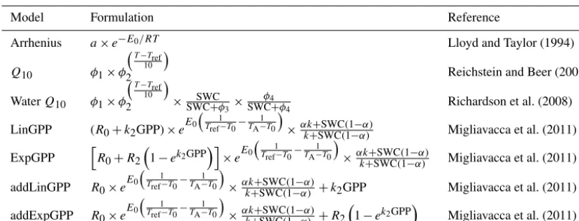
Table 2.Respiration model formulations commonly used in the environmental science community.
Model Formulation Reference
Arrhenius a×e−E0/RT Lloyd and Taylor (1994)
Q10 φ1×φ
T−Tref
10
2 Reichstein and Beer (2008)
WaterQ10 φ1×φ
T−T
ref 10
2 ×SWCSWC+φ3 × φ4
SWC+φ4 Richardson et al. (2008)
LinGPP (R0+k2GPP)×e E0
1
Tref−T0−TA1−T0
×αk+SWC(1−α)
k+SWC(1−α) Migliavacca et al. (2011) ExpGPP hR0+R21−ek2GPPi×eE0
1
Tref−T0− 1
TA−T0
×αk+SWC(1−α)
k+SWC(1−α) Migliavacca et al. (2011) addLinGPP R0×e
E0
1
Tref−T0−TA1−T0
×αk+SWC(1−α)
k+SWC(1−α) +k2GPP Migliavacca et al. (2011) addExpGPP R0×e
E0
1
Tref−T0− 1
TA−T0
×αk+SWC(1−α) k+SWC(1−α) +R2
1−ek2GPP
Migliavacca et al. (2011)
a,E0,φ1,φ2,φ3,φ4,R0,R2,k,k2andαare model parameters that can be optimized.
(a) (b)
Figure 4.Effect of adding noise to the original signal on the prediction capacity for GEP, KRR, RF, SVM and ANN. The first panel contains the evolution of mean modelling efficiency (MEF) values from 20 independent runs for each increasing level of noise. MEF is computed after learning from a data set of 200 data points and validating against 1000 data points containing noise. The second panel shows the evolution of mean MEF values from 20 independent runs for each increasing level of noise where MEF is computed after learning from a data set of 200 data points and validating against noise-free 1000 data points generated from Eq. (14).
and compared with those of the GEP-extracted models. The comparison is done in terms of MEF as a number of model parameters were not available and CEM could not be com-puted.
3.2.4 GEP in the context of other known ecological models: real observational data
A comparison was done between the GEP-built models and some common literature respiration models with different structures and driving variables that were also optimized us-ing CMA-ES. The optimization was performed for each res-piration data set and its candidate drivers and parameters (Table 2). The structures and prediction performances of the GEP models were then compared with those of the optimized literature models.
4 Results
4.1 Artificial experiments
In the first artificial experiment the GEP approach is used to verify whether it can reconstruct prescribed functions. Fol-lowing the training of the 20 independent GEP runs, the ini-tial functions were successfully reconstructed for all 10 equa-tions defined in Sect. 3.1.
For theQ10 model artificial test, the following structure
was finally selected:
Reco=0.35×2.5(0.01Tair), (21)
with a validation MEF value>0.99.
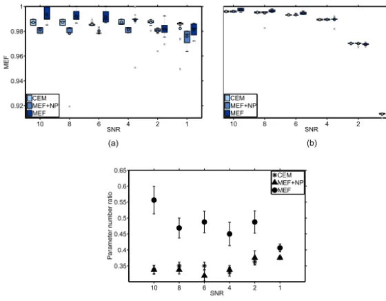
in-(a) (b)
(c)
Figure 5.Effects on modelling performance and parameter number caused by choice of fitness function during GEP training for artificial noisy data generated by Eq. (14), where MEF is defined in Eq. (1) and CEM is defined in Eq. (3).(a)Mean MEF when validated against noisy data after 20 GEP runs with different fitness functions.(b)Mean MEF when validated against noise-free data after 20 GEP runs with different fitness functions.(c)Ratio of predicted number of parameters to true number of parameters after 20 GEP runs with different fitness functions.
creasing noise contamination. This was expected, as none of the methods should fit the noise added to the signal.
Figure 4b shows MEF values equivalent to Fig. 4a but ap-plied to noise-free data points of the validation set, in order to compare GEP outputs to the “true” structure underlying the artificial data set. In this set-up, the MEF values remained relatively constant across SNR values above 2. When the SNR level was set to 1, predictions for all investigated ma-chine learning methods, except for GEP predictions, show decreased fitness, with MEF values decreasing to a minimum of 0.8.
In order to verify the effects of changing the fitness func-tion from MEF to CEM, we compare the distribufunc-tions of MEF values for all runs for all studied SNRs. Figure 5 ex-emplifies outputs for Eq. (14); Fig. 5a shows a drop in the prediction capacity of the GEP models with noise increase for all types of fitness functions when compared with noise-infused data. This contrasts with the reduced MEF assessed against original data, where a slight drop in MEF with noise increase for the MEF optimization structures was seen, and where the CEM optimized structures show stability in MEF with noise. The new CEM leads to a reduced number of re-turned parameters compared to MEF (Fig. 5c), as well.
4.2 Measured ecosystem CO2fluxes
Applying GEP to the Alice Holt data set yielded a series of model structures for each respiration type. The returned
model structures after bias corrected back-transformation are illustrated in Eqs. (22)–(28).
Reco=1.2 log(T−10)0.8×e
GPPs
T−10
, (22)
Rabove=1.1SWC0.3×e(0.1GPPs), (23) Rsoil=0.04e
1.1T−0.104+1.6SWC
, (24)
Rroot=1.1e
0.9GPPs−6.8
T−10 , (25)
Rmyc=0.001T−1.102 ×e(1.6T−10) SWC
, (26)
Rsoila=0.01e
0.8T0.6
−10+2.6SWC
, (27)
Rsoilh=0.8e
0.6GPPs−2.4
T−10 , (28)
where GPPs is gross primary production that has been
smoothed using the SSA method with a 60-day window; T−10 is soil temperature measured at 10 cm depth; and
SWC is volumetric soil water content. The corresponding cross-validation MEF values are given in Table 3, indicating a range of capacities for GEP models to represent different respiration types.
Whilst GEP-derived models may differ between respira-tion types, there are a number of equivalent models for differ-ent respiration compondiffer-ents.Rsoil andRsoila were described
by identical model structures (but distinctive parameter val-ues), andRrootandRsoilh were described by similar (but not
2
2
2
2
2 2 2
Figure 6.Observed and predicted outgoing CO2fluxes; 613 time steps of daily averaged CO2effluxes for 2 years at the Alice Holt oak forest
site. The predicted values are generated with the models automatically built by the GEP approach with the settings given in Table 1 for the following types of respiration,Reco,Rabove,Rsoil,Rroot,Rmyc,Rsoila, andRsoilh, and back-transformed with a smear term bias correction.
The models are given in Eqs. (22)–(28).
Table 3.Modelling performance for all extracted model structures after cross-validation over 90 cases.
Respiration type MEF σMEF Equation
Reco 0.57 0.13 (22)
Rabove 0.31 0.23 (23)
Rsoil 0.79 0.04 (24)
Rroot 0.59 0.08 (25)
Rmyc 0.39 0.28 (26)
Rsoila 0.82 0.05 (27)
Rsoilh 0.52 0.08 (28)
The highest performance in terms of MEF value was recorded forRsoilaand forRsoil, that is, 0.82 and 0.81
respec-tively. The lowest capacity of process representation, with an MEF value of 0.28, was recorded forRabove(Table 3),
pos-sibly because this specific component would need to include active versus inactive periods determined by dormancy and leaf fall (i.e. seasonality in this deciduous forest). A compar-ison of the predicted values and observed fluxes for all types of respiration can be seen in Figs. 6 and 8. Figures 7 and 9 show the effects of the three different types of bias
correc-tion on the global signal reconstruccorrec-tion and prediccorrec-tion capac-ity with MEF values computed in a cross-validation manner. For all respiration types, exceptRsoil, doing the second type
of bias correction with a smear term improved the predic-tion capacity. Although forRsoil it seems that doing no bias
correction gives a higher MEF value, we chose to keep the model including the smear term.
In order to explore the capacity of the GEP models gener-ated for theRecocomponents to recreate the larger,
Figure 7.Observed and predicted outgoing CO2fluxes; 613 time steps of daily averaged CO2effluxes for 2 years at the Alice Holt oak
forest site. The predicted values are generated with the models automatically built by the GEP approach with the settings given in Table 1 for the following types of respiration,Reco,Rabove,Rsoil,Rroot,Rmyc,Rsoila, andRsoilh, and back-transformed with three types of residual
biascorrection terms:smear term,naive, andlog-normal term.
only get selected in the models built for those specific com-ponents.
The residuals depict some remaining patterns (Figs. 11 and S3) and the null hypothesis of normal distribution was rejected for all seven respiration component residuals at the 5 % significance level with the one-sample Kolmogorov– Smirnov test. Hence, we might expect additional information that could be extracted from the residuals. In order to check whether the remaining structure was missed in the first train-ing routine because of impostrain-ing a multiplicative form in the models by log-transforming the target data, we performed GEP runs on the residuals and combined the models. The im-provement in overall modelling performance is minimal, yet model structures become overly complex. The capacity of the GEP approach to retrieve new information from the residu-als is illustrated in Fig. 13 in comparison with that of the other MLM presented in Sect. “Alternative machine learning methods”. When correlation values were computed between the candidate drivers and the residuals, no significant linear correlations were found (Figs. S5 and S6).
4.2.1 Model transferability
We investigated the capacity of each extracted model struc-ture (Eqs. 22–28) to represent a component of Reco not
seen in the training procedure. This was done by means of new CMA-ES optimization steps. The new prediction per-formances are illustrated in Table 4.
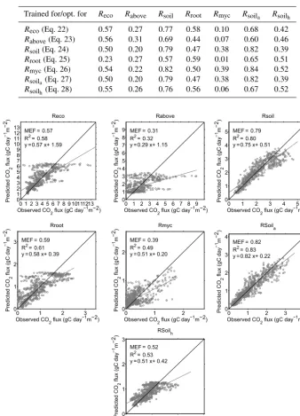
After optimization, none of the structures show an overall best MEF for all theReco components (i.e. we clearly
can-not identify an optimal general model). However, we iden-tify certain model structures that tend to perform overall bet-ter than others. This is the case for theRmycmodel (Eq. 26).
It can also be seen that after the individual model optimiza-tions, the structures forRecoand that forRsoila have similar
prediction capacities.
val-Table 4.Average validation MEF performance for all extracted model structures when re-optimized against all other respiration CO2flux observations.
Trained for/opt. for Reco Rabove Rsoil Rroot Rmyc Rsoila Rsoilh
Reco(Eq. 22) 0.57 0.27 0.77 0.58 0.10 0.68 0.42
Rabove(Eq. 23) 0.56 0.31 0.69 0.44 0.07 0.60 0.46
Rsoil(Eq. 24) 0.50 0.20 0.79 0.47 0.38 0.82 0.39
Rroot(Eq. 25) 0.23 0.27 0.57 0.59 0.01 0.65 0.51
Rmyc(Eq. 26) 0.54 0.22 0.82 0.50 0.39 0.84 0.52
Rsoila(Eq. 27) 0.50 0.20 0.79 0.47 0.38 0.82 0.39
Rsoilh(Eq. 28) 0.55 0.26 0.76 0.56 0.06 0.67 0.52
Figure 8.Observed and predicted outgoing CO2fluxes; 613 time steps of daily averaged CO2effluxes for 2 years at the Alice Holt oak forest
site. The predicted values are generated with the models automatically built by the GEP approach with the settings given in Table 1 for the following types of respiration,Reco,Rabove,Rsoil,Rroot,Rmyc,Rsoila, andRsoilh, and back-transformed with a smear term bias correction.
The models are given in Eqs. (22)–(28).
ues when compared to the original observations for Reco, Rabove, Rsoil, Rroot, Rmyc, Rsoila, and Rsoilh. For all other
cases, the performance is in the same range for all methods, but the GEP-derived models have the lowest mean MEF val-ues. Figure 13b shows that when all MLMs were trained on the residuals obtained from comparing the GEP outputs with the observations, the GEP approach has the lowest capacity
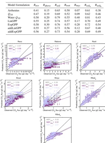
Table 5.Average validation MEF performance for CMA-ES optimized selected literature model formulations when compared with respira-tion CO2flux observations.
Model formulation Reco Rabove Rsoil Rroot Rmyc Rsoila Rsoilh
Arrhenius 0.41 0.15 0.65 0.50 0.07 0.61 0.38
Q10 0.47 0.19 0.69 0.52 0.09 0.62 0.46
WaterQ10 0.50 0.20 0.79 0.55 0.40 0.81 0.43
LinGPP 0.55 0.25 0.74 0.57 0.17 0.70 0.49 ExpGPP 0.58 0.30 0.76 0.57 0.20 0.72 0.54 addLinGPP 0.55 0.27 0.73 0.56 0.12 0.67 0.48 addExpGPP 0.56 0.27 0.73 0.54 0.20 0.69 0.49
Figure 9.Observed and predicted outgoing CO2fluxes; 613 time steps of daily averaged CO2effluxes for 2 years at the Alice Holt oak forest site. The predicted values are generated with the models automatically built by the GEP approach with the settings given in Table 1 for the following types of respiration,Reco,Rabove,Rsoil,Rroot,Rmyc,Rsoila, andRsoilh, and back-transformed with three types of residual
biascorrection terms:smear term,naive, andlog-normal term. The figure contains the MEF values for each type of bias correction in each respective colour.
4.2.2 Comparing with literature models
Lastly, the GEP-generated models were compared with some of the most commonly used literature models for describing respiration. The resulting MEF values obtained after indi-vidual parameter optimization using the CMA-ES procedure for each literature model are given in Table 5. The literature
model structure that performed best overall in terms of pre-diction capacity measured as MEF is the WaterQ10 model
respira-Figure 10.Observed versus predictedRecocomponent fluxes, where predicted values are computed as derived fluxes based on the GEP
models given in Eqs. (22)–(28) that were trained on 500 data points (d.p.) of daily mean values of variousRecocomponents.
-1
--1
--1
--1
--1
--1
--1
-Figure 11.Residuals computed for smear term bias corrected back-transformed GEP models for various types of CO2respiration fluxes after
Figure 12.Observed CO2fluxes and one set of 113 predicted values given by the some common machine learning methods (MLMs) after
training on 500 data points and after smear term bias corrected back-transformation.
(a) (b)
Figure 13.Machine learning methods (MLM) prediction performance for all respirations components(a)and for the residuals(b)resulting from the GEP trained models after smear term bias corrected back-transformation. The MEF values obtained for validation by all the MLM methods forReco,Rabove,Rsoil,Rroot,Rmyc,Rsoila,Rsoilh.
tion types, the highest MEF values are generally recorded by the GEP models.
As the studied literature models performed best in mod-elling Rsoil, we focus on contrasting GEP model results
with literature model outcomes for this ecosystem respira-tion component. Of all models included, the GEP model and Q10 model including SWC dependency captured
sea-sonal variability best, but no model satisfactorily represented
short-term CO2 flux variations (Fig. 15a). All models show
the largest range of residuals for the months May to July in 2008, and June/July in 2009 (Fig. 15b), with the two best-performing models (GEP and WaterQ10) having the
Figure 14.MEF validation values for literature models and for the best GEP model in terms of MEF at each respiration level. Each
Recoflux component is shown in a separate colour.
5 Discussion
5.1 On the GEP method
In this work, the primary reason for the artificial experiments was to obtain a better understanding of the capacity of GEP to solve symbolic regression types of problems. We put an emphasis on GEP performance in the presence of noise. This aspect was important, given that monitoring data from ter-restrial ecosystem CO2 effluxes are typically contaminated
by sometimes substantially large random uncertainties and measurement noise. In the case of NEE flux measurements, Lasslop et al. (2008) and Richardson et al. (2008) show that the measurement error typically scales with the magnitude of the flux, leading us to simulate that type of situation by adding noise that scales with signal to an already known function, Eq. (14). The results show that all the studied meth-ods are stable in the presence of noise in the training set. These results increase our confidence in the predictions gen-erated by studied machine learning methods; in particular, GEP-derived modes can tolerate SNRs of 1. Considering that the SNR in theRecoobservations (if noise is only considered
as a random error) is probably larger than 4, which is where the curve starts decreasing in Fig. 4, the noise presence in the data should not influence the automated model construction process and the real signals should be accurately captured when data uncertainties follow the pattern described here. On the other hand, forRsoil and other CO2fluxes measured
with other techniques, the magnitude and the distribution of the uncertainty can be different (Ryan and Law, 2005; Pérez-Priego et al., 2015), and we cannot state what the response of the present MLM is in the presence of different types of uncertainties and measurement noise.
Our findings illustrate that the selection of CEM over MEF as a fitness function for optimization has a minor effect on the global mean MEF (Fig. 5). We also notice that due to
apply-ing constraints on the presence of structures in the residuals and the length of the parameter vector, the final mean number of parameters is lower when CEM is chosen.
Limitations
One of the critical aspects in our work is that GEP, as imple-mented here, can only represent and derive “n→1” types of response functions. We are not able to generate model structures that encode e.g. system-intrinsic dynamics like feedback loops, which are expected from our current under-standing of biogeochemical cycles in terrestrial ecosystems (Ehrenfeld et al., 2005; Friedlingstein et al., 2006). Hence, we believe GEP is suitable for e.g. understanding and de-scribing the sensitivities and non-linear responses to changes in hydro-meteorological drivers, but fails to represent more complex carbon or soil water dynamics. Pools and pool trans-fers cannot be introduced currently in the input, unless the inflow–outflow equations are known and can be included in the set of functions that can participate in the evolution.
Lagged responses can only be detected if the number of lags from a driver is correctly included in the input, which already implies sufficient knowledge of their existence and behaviour. Whilst in the current implementation of the GEP algorithm, shifts in conditions and responses cannot be en-coded or detected, these could be addressed with the inclu-sion of a conditional operator in the set of functions encoded in the GEP evolution individuals.
Nevertheless, it would be fair to mention that the same lim-itations can affect the results of the other MLM and empiri-cal models presented in this paper. A clear advantage ANN, RF and SVM have though over the GEP symbolic regression construction is the fact that when the target variable presents a skewed distribution, log-transforming of the target data is recommended for regression types of methods, such as GEP (Keene, 1995), whereas there is no effect on the prediction capacity of the other MLM as far as we are aware. Moreover, such a log-transformation needs a back-transformations that might induce a bias if the right correction is not performed (Manning, 1998). For these reasons, in cases where less steps in obtaining predictions are desired and no mathematical ex-pression of the models needed to obtain the predictions are needed, non-GEP approaches might be recommended.
5.2 The value of GEP for modelling ecosystem respiration fluxes
We automatically generated a series of model structures to describe terrestrial CO2 respiration fluxes (Eqs. 22–28)
with the GEP approach. Most of these structures (five out of seven) were of rather low complexity, requiring only four free parameters and allowing for further interpretation. The most complex structure is found for theRmyc
(a)
(b)
Figure 15.DailyRsoilfluxes(a)illustrated in the context of the 2 studied years and residual values(b)of the total soil daily CO2outgoing
fluxes as simulated by the investigated literature models and the GEP emerged model after smear term bias corrected back-transformation. The fluxes shown here are the real flux measured at the site and the predicted fluxes generated according to the GEP model and some of the models used in the environmental science community. The centre of the plots in the second row is−1. The scale of the fluxes is given in gC m−2day−1.
Interestingly, the models derived for Reco and Rsoil are
structurally very similar. That is also the case ofRroot and
heterotrophic respiration, where the difference lies in the set of parameters and the added presence of an intercept in the formulation of theRsoilhmodel. This finding suggests a
con-sistency in the response of the Rsoil components to their
drivers, considering that the separation of the Rsoil into its
components might still lack accuracy (e.g. Hanson et al., 2000; Kuzyakov, 2006; Subke et al., 2006; Heinemeyer et al., 2011).
When we compared the GEP-derived models with the community established semi-empirical models from a struc-tural point of view, we found that they shared some key fea-tures for temperature dependencies of CO2fluxes, which are
typically captured by exponential relationships, but reveal some previously unconsidered dynamics as well.
A major difference was in the response of the respiration components to SWC, where the GEP models often chose SWC as one of the drivers. Moreover, the GEP models of-ten contained an exponential dependency, i.e. there are only certain parts of the signal that are strongly sensitive to vary-ing SWC. We believe that the exponential dependency of
ter-restrial ecosystem respiration components on SWC is a very intuitive pattern that has not yet been reported in the literature and requires further exploration.
Another difference we found was the strongly seasonal re-sponse of the respiration components to GPP, possibly as a proxy to light and vegetation availability which were not in-cluded in the set of candidate predictors.
Considering that GEP identified plausible models that are very different structurally from previously reported semi-empirical models, still yielding equivalent or better mod-elling performance, the validity of the conventional semi-empirical models can be questioned. Nevertheless, we do be-lieve that there is a need for more in-depth analysis for de-termining whether the GEP described processes make actual biological sense and whether the selected drivers and their interactions represent true processes and responses.
5.3 Data quality
obtained from derivations, the measurement error will also increase, and the partition of a clear signal existing in the observations is not sufficient for constructing a good model with GEP.
5.4 High-frequency variability
All GEP-generated models underestimated the high respi-ration fluxes (Fig. 8) and typically did not capture the fast responses. This phenomenon was in some cases a system-atic pattern, and sometimes affected only certain times of the year. Similarly, semi-empirical models struggled to ade-quately simulate CO2flux peaks and in some cases monthly
flux averages (Fig. 15).
A more in-depth comparison of all the GEP and conven-tional respiration models, based on a timescale-dependent as-sessment of model–data mismatch (Mahecha et al., 2010), could help to further elucidate the problem and clarify some of the strengths and weaknesses of the different modelling approaches, especially when seasonal mismatches appear. Nevertheless, a detailed timescale-dependent assessment is beyond the scope of this study, and for such an analysis, the current time series are simply too short.
The question is whether the GEP method lacks the abil-ity to build models that correctly represent the processes and their fast dynamic responses, or whether the candidate drivers and the observations used for their representation are simply not sufficient for generating representative models. In the end, the response of Rsoil andReco to external drivers
might be too complex to describe solely with the currently available measurements and with the selected drivers.
We believe that the consistent underestimation of fast re-sponses was partly due to surface moisture affecting litter decomposition and fungal activity, as soil moisture was only monitored over the average 8 cm surface, with the top few centimetres most likely presenting the highest activity and partly due to some potential processes/drivers like lags be-tween GPP and respiration (Hölttä et al., 2011) or phenology (Migliavacca et al., 2015) that were not specifically included in the learning process.
Another explanation for missing some of the (high flux) variability could be in our choice of fitness function. As we decided to penalize during the learning process for structures with many parameters, it is likely that some structures were eliminated early on during this process, even though they may be well suited for describing a given process from a modelling efficiency point of view. However, this is a case of trade-off between a good fit and structural simplicity, and in our approach, we decided that simplicity of structure, i.e. the possibility of interpretation, is a very important asset.
We explored as well the possibility of the underestima-tion of the carbon flux variability being caused by the log-transformations applied to the observations. It could have been the case that the log-transformations excluded inter-esting components of the model structures by forcing the
method to build multiplicative models. Nevertheless, when the GEP was run again on the residuals, without log-transforming, no new meaningful information was retrieved, indicating that multiplicative models were sufficient for re-constructing theRecocomponents present in this study.
5.5 Equifinality
Table 4 shows that when optimizing the parameters for all structures, the prediction performance becomes similar, which leads to the question of equifinality of dynamical sys-tems, where different models that try to capture their struc-ture might have different formulations but represent the same response.
A critical question for the applicability of any ecosys-tem model is whether the model structure is more important than the parameterization of a given “best” model. For this question to be addressed, however, we need a larger sam-ple of ecosystem types representative of different types of re-sponses where we can explore the importance of the obtained structures and their parameter sets.
5.6 GEP models in the context of other machine learning methods
The comparison of GEP-generated models and machine learning methods showed a narrow range of predicted fluxes (Fig. 13). The analysis of training all the MLMs on the GEP residual output showed that the GEP approach is not able to retrieve any new meaningful structural components, but that the remaining MLMs are much better at reconstructing the signal left in the residuals. This indicates that although the GEP is actually a reliable MLM when it comes to re-constructing the underlyingReco fluxes and is not prone to
overfitting, it could be that the current set-up of the GEP is not sufficient for an exhaustive description of those fluxes, or that it might be overly strict on the complexity of models compared to other MLMs. The GEP approach has, neverthe-less, the benefit of producing mathematical model structures that can be the basis for future interpretation.
6 Conclusions and outlook
Overall, our results suggest that the GEP approach is a poten-tially powerful tool of reverse engineering, particularly help-ful for building ecological models when there is a minimum of a priori system understanding. We exemplified this con-ceptually using artificial data, but also show that GEP always yields as good or better results compared to conventionally used models in the case of ecosystem respiration. Based on data from a long-term monitoring site of different respira-tory fluxes, and using GEP as a reverse engineering tool, we found new structures for modelling Reco components. The
SWC are interpreted, indicating that conventional respiration models might have to be revised. At the same time, we found that when the GEP-derived models are mutually compared, there are sufficient structural particularities for each terres-trial respiration type so as to not allow for the formulation of a generalRecolaw. More research is needed on a larger set of
sites to identify widely usable models and for their interpre-tation. A particular matter of concern is the apparent equifi-nality of selected model structures, indicating that many re-sponse functions are yielding predictions of almost similar quality. A study of multiple sites would enable an investi-gation of whether specific ecosystem types result in similar model structures, or whether response functions apply across contrasting ecosystem types.
The current study has also revealed methodological as-pects that could be improved. In particular, we found the inclusion of a parameter optimization step very helpful to further test the transferability of model structures. But this approach could be potentially integrated into the GEP evolu-tion. More specifically, we think that the next development of GEP could include the parameter optimization as an interme-diate step before selection during each evolution generation (Ilie et al., 2017). In this way, a model structure could be cho-sen according to not only the current state of parameters, but also according to its potential, and convergence to a global solution might be achieved faster.
Appendix A: Glossary
expression tree binary tree used to represent algebraic expressions
gene set of characters of fixed length that encodes an expression tree
chromosome individual used in automatically evolving an optimal solution comprised of a set of genes that are connected with a binary operation (e.g.+ × −)
GEP geneexpressionprogramming, machine learning method that evolves chromosome structures with the purpose of minimizing a cost function
genetic operator operator that produces changes in the structure of a chromosome and the expression tree it encodes by altering the strings representing composing genes (e.g. mutation, inversion, recombination) evolution the process of producing an optimal solution by GEP through
generation time step of an evolution
genetic operator rate probability of a genetic manipulation occurring during a generation
population total set of chromosomes that participate at a certain step in the evolution of an optimal solution in the GEP approach
CMA-ES covariance matrix adaptation evolutionary strategy
MLM machinelearningmethod that can produce predicted values based on a training set
ill-posed problem a problem for which the solutions might not be unique or unstable, also known as an inverse problem reproduction process of generating new individuals for a new generation starting from the present-generation
individuals after they go through structure modification and fitness-based selection
individual GEP entity that is a component of a population during a certain step of the evolution process. Also known as a chromosome.
gene head initial section of the string that comprises a GEP gene, containing a combination of characters that map to predictors and possible functional transformations
gene tail end section of the string that comprises a GEP gene, containing only characters that map to predictors
solution finally selected model structure resulting from a GEP run