Visualization of Pareto Front Points when Solving Multi-objective
Optimization Problems
Olga Kurasova
1,2, Tomas Petkus
1, Ernestas Filatovas
21 Lithuanian University of Educational Sciences Studentų str. 39, LT–08106 Vilnius, Lithuania e-mail: [email protected], [email protected]
2 Vilnius University
Universiteto str. 3, LT–01513 Vilnius, Lithuania e-mail: [email protected]
http://dx.doi.org/10.5755/j01.itc.42.4.3209
Abstract. In this paper, a new strategy of visualizing Pareto front points is proposed when solving multi-objective optimization problems. A problem of graphical representation of the Pareto front points arises when the number of objectives is larger than 2 or 3, because, in this case, the Pareto front points are multidimensional. We face the problem of multidimensional data visualization. The visualization strategy proposed is based on a combination of clustering and dimensionality reduction. Moreover, in the obtained projection of the Pareto front points onto a plane, the points are marked according to the Euclidean distance of multidimensional points, corresponding to the points visualized, from the ideal point. In the experimental investigation of the paper, neural gas is used for data clustering, and multidimensional scaling is applied to dimensionality reduction, as well as to visualizing multidimensional data. The strategy can be implemented in a decision support system and it would be useful for a decision maker, who needs to review and evaluate many points of the Pareto fronts, for example, obtained by genetic algorithms.
Keywords: Multi-objective optimization; visualization; clustering; Pareto front; ideal point; neural gas; multidimensional scaling; genetic algorithms; NSGA-II.
1. Introduction
Problems arising in the real world applications are often multi-objective. Usually, objectives are contradictory. It is necessary to find trade-off solutions, i.e., a so-called Pareto solution set has to be discovered. Pareto solutions are the solutions that cannot be improved in any objectives without deteriorating in at least one of other objectives. The values of objectives for the Pareto solutions form a Pareto front.
When solving multi-objective optimization problems, a decision maker plays an important role. He/she has to select preferable solutions from a set of the Pareto solutions. If only numerical values of the solutions and objectives are given to the decision maker, he/she faces difficulties in choosing the preferable solutions, especially, if the amount of solutions is large, for example, when using genetic algorithms in search of the Pareto solutions.
It is important to have some tools for a graphical representation of the Pareto front in order to facilitate
the choice of solutions for the decision maker. If the number of objectives is equal to 2 or 3, the graphical representation of the Pareto front is simple. The values of objectives can be presented in a 2D or 3D Cartesian coordinate system. Difficulties arise when the number of objectives is larger, i.e., we face the visualization of multidimensional data.
Moreover, if algorithms for the multi-objective optimization find many Pareto solutions, it is difficult for the decision maker to evaluate all the solutions. So, it is purposeful to cluster the solutions and evaluate only the representatives of the clusters, regarding that all the solutions in a cluster are similar.
solutions faster without looking for numerical values of the Pareto front points.
The rest of the paper is organized as follows. Section 2 reviews the techniques for visualizing the Pareto front points. In Section 3, a new strategy of visualization is proposed and described for evaluating the solutions obtained. The visualization results, obtained by the strategy proposed, when solving some multi-objective optimization test problems, are presented in Section 4. Conclusions are drawn in the final section.
2. A review of visualizing the Pareto front
points
At first, a multi-objective optimization problem is
introduced. Let us have 𝑚 objectives, described by the
functions 𝑓1(𝑋),𝑓2(𝑋), … ,𝑓𝑚(𝑋), where 𝑋=
(𝑥1,𝑥2, … ,𝑥𝑛) is a vector of variables (decision
vector), 𝑛 is the number of variables. A
multi-objective minimization problem is formulated as follows:
min𝑋∈𝐃𝐅(X) = [𝑓1(𝑋),𝑓2(𝑋), … ,𝑓𝑚(𝑋)] . (1)
Here 𝐃 is a bounded domain (feasible set, decision
space) in the 𝑛-dimensional Euclidean space ℝ𝑛;
𝐅(𝑋)∈ ℝ𝑚 is a vector of objective functions. Each
vector 𝑋∗∈ 𝐃 is called a feasible solution. The vector
𝐙∗=𝐅(𝑋∗)∈ ℝ𝑚 for a feasible solution 𝑋∗ is called
an objective vector. A set of the objective vectors composes the so-called feasible criterion space (feasible region).
In the multi-objective optimization, there exists no feasible solution that minimizes (maximizes) all the
objective functions 𝑓1(𝑋),𝑓2(𝑋), … ,𝑓𝑚(𝑋)
simultaneously, in the case, where the objectives are contradictory. Here the Pareto optimal solutions are
very important. The solution 𝑋∗∈ 𝐃 is Pareto optimal
(non-dominated), if and only if there does not exist another solution 𝑋 ∈ 𝐃, such that 𝐅(𝑋)≤ 𝐅(𝑋∗), and
𝑓𝑖(𝑋) <𝑓𝑖(𝑋∗) for at least one objective. The set of all
the Pareto optimal solutions is called a Pareto set. The region defined by the value of all objectives for all the Pareto set points is called a Pareto front.
When solving multi-objective optimization problems arising in the real world, usually determination of the exact Pareto front is impossible, because the front is an infinite set. Therefore, a discrete approximation is searched. For simplicity, we call this approximation a Pareto front. The point
𝐅id=�𝑓
1id,𝑓2id, … ,𝑓𝑚id� ∈ 𝐙𝑚 is called an ideal
objective vector (point), where 𝑓𝑖id(𝑋) =
min𝑋{𝑓𝑖(𝑋) |𝑋 ∈ 𝐃}. In general, the ideal objective
vector corresponds to a non-existent solution. The Euclidean distance between a point of the Pareto front and the ideal point is smaller, the solution is more preferable for a decision maker, when the importance of objectives is the same.
There are many algorithms for solving multi-objective optimization problems [1], [2], [3], [4], [5]. Recently, the algorithms, based on evolutionary computation, have been rapidly developed. They are called evolutionary multi-objective optimization (EMO) algorithms. The particularity of the algorithms is that they generate a large amount of solutions. So, a decision maker faces a problem of reviewing the solutions obtained, because he/she has to spend a lot of time reviewing all solutions.
One of the most popular algorithms is a non-dominated sorting genetic algorithm II (NSGA-II) [6]. The algorithm is used in the experimental investigation of the paper. The main advantage of the algorithm is that it manages to solve the problems with many objectives and it is not necessary to take into account the geometrical characteristics of the Pareto fronts, such as concave, convex, and disconnecting. It should be noted that solutions, found by NSGA-II, are only an approximation of Pareto solutions, but not the exact Pareto solutions. The paper does not focus on searching for the true Pareto solutions, it is aimed at visualization of points of the Pareto front or its approximation.
Thus, in the multi-objective optimization, it is important to find Pareto optimal solutions. Moreover, when solving multi-objective optimization problems, a decision maker plays an important role. The task of the decision maker is not easy. He/she has to select the most preferable solution from a set of the Pareto optimal solutions and to make the final decision. When only the numerical values are presented to the decision maker, he/she faces a difficulty to select a solution such that satisfies his/her preferences, especially if the numbers of variables and objectives as well as that of the Pareto solutions are large. Proper visualization techniques can be helpful to solve the problem.
Visualization is a graphical representation of information allowing a viewer to understand the information content more easily. Visualization techniques are applied in different areas and many methods are developed. A comprehensive review of methods and applications is presented in [7]. The most popular multidimensional data visualization methods are a scatter plot, a matrix of scatter plots, multidimensional scaling [8], parallel coordinates [9], and self-organizing maps [10].
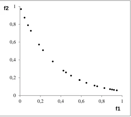
Some ways of visualizing the Pareto front points have also been proposed. A simple way of visualization exists for bi-objective optimization
problems, i.e., if the number of objectives is equal to 2
(𝑚= 2). In this way, the values of objectives 𝑓1(𝑋∗)
and 𝑓2(𝑋∗) are plotted in the Cartesian coordinate
Figure 1. Points of the Pareto front in the Cartesian coordinate system in a bi-objective case
If the number 𝑚 of objectives is equal to 3, it is
possible to plot the Pareto front in a 3D Cartesian coordinate system, but interpretations of the results are
more difficult than in the case, where 𝑚= 2,
especially if there is no possibility of rotating the coordinate system.
An even greater problem arises when there are more than three objectives, because the ordinary Cartesian coordinate system is insufficient. It is necessary to search for more sophisticated ways that enable us to visualize multidimensional points
𝑌1,𝑌2, … ,𝑌𝑘 , where 𝑌𝑖= (𝑦𝑖1,𝑦𝑖2, … ,𝑦𝑖𝑚) .
Multidimensional points are called those points, the dimension 𝑚 of which is higher than 2 or 3.
In solving multi-objective optimization problems,
in case the number 𝑚 of objectives is larger than 2 or
3, the Pareto front consists of𝑚-dimensional points
𝑌1,𝑌2, … ,𝑌𝑘, where 𝑌𝑖=�𝑓1(𝑋𝑖∗),𝑓2(𝑋𝑖∗), … ,𝑓𝑚(𝑋𝑖∗)�, 𝑌𝑖∈ ℝ𝑚, 𝑖= 1, … ,𝑘; 𝑘 is the number of points of the
Pareto front.
Some techniques of the Pareto front visualization are reviewed in this paper. Parallel coordinates are used for visualizing the Pareto front in [11]. The coordinate axes are shown there as parallel lines that represent the coordinates of multidimensional points.
An 𝑚-dimensional point is represented as an 𝑚 −1
line segment, connected to each of the parallel lines at the appropriate coordinate value.
Visualization of the Pareto front by the self-organizing map (SOM) is investigated in [12]. SOM is a type of neural network used for data clustering and visualization [8]. In the paper, not only the Pareto front, but also variables are visualized by SOM. In addition, a hierarchical agglomerative algorithm, based on the SOM-Ward distance, is used for clustering the points mapped on SOM.
Instead of the traditional plane SOM, a spherical self-organizing map is proposed as a visualization technique of Pareto solutions in [13]. Neurons in a spherical SOM are placed in a geodesic dome. A
geodesic dome is a triangulation of a polyhedron that produces a close approximation to a sphere. Yoshimi et al. [13] ascertained that the spherical SOM allows us to find similarities in data otherwise undetectable by plane SOM.
Another graphical representation, called level
diagrams, is proposed in [14] for 𝑚-dimensional
Pareto front analysis. Level diagrams consist of the representation of each objective and variable in separate diagrams. This technique is based on the classification of Pareto front points according to their proximity to the ideal point, measured with a specific norm of normalized objectives and synchronization of objective and variable diagrams. In [14], the parallel coordinates and the scatter plot matrix are applied as well.
The so-called hyper-space diagonal counting (HSDC) method is developed in [15]. The method enables an intuitive and meaningful visualization capability of multi-objective optimization problems, when the number of objectives is higher than 2 or 3.
Visualization of Pareto sets in evolutionary multi-objective optimization is presented in [16]. The main characteristic of this technique is that preservation of Pareto dominance relations among the individuals be as good as possible. The authors have proposed a
two-stage mapping of 𝑚-dimensional points of the Pareto
front. The first stage is mapping of the points into a plane (2D space), and the second stage is mapping of the dominated points.
Interactive decision maps are introduced and applied to visualize the Pareto front in [17], [18]. The main feature of an interactive decision map is a direct approximation of the Edgeworth-Pareto Hull (EPH) that is used for a fast interactive visualization of the Pareto front as the fronts of two-objective slices of EPH.
3. The visualization strategy proposed
As mentioned above, if the number 𝑚 of
objectives is higher than 2 or 3, the points of the
Pareto front are multidimensional and they can be visualized by the methods of multidimensional data visualization [7], for example, by multidimensional scaling and principal component analysis. Moreover, if the number 𝑘 of Pareto solutions is rather large, it is reasonable to cluster the points and, later, to visualize the representatives of clusters. Especially the genetic algorithms, for example, one of the popular algorithms NSGA-II, generate many solutions and it is difficult to review them for a decision maker without an additional graphical representation. Moreover, after reviewing some solutions from a cluster, the decision maker will gain information about the particularity of solutions of the whole cluster.
The new strategy for visualizing points of the Pareto front proposed here is as follows:
0 0,2 0,4 0,6 0,8 1
0 0,2 0,4 0,6 0,8 1
f2
1. The Pareto solutions 𝑋1∗,𝑋2∗, … ,𝑋𝑘∗ and points of the Pareto front (or its approximation)
𝑓1(𝑋𝑖∗),𝑓2(𝑋𝑖∗), … ,𝑓𝑚(𝑋𝑖∗), 𝑖= 1, … ,𝑘, are found
by using any methods for multi-objective
optimization, where 𝑘 is the number of points of
the Pareto front. A set of multidimensional points
𝑌1,𝑌2, … ,𝑌𝑘 is formed, where 𝑌𝑖=�𝑓1(𝑋𝑖∗),𝑓2(𝑋𝑖∗), … ,𝑓𝑚(𝑋𝑖∗)� , 𝑖= 1, … ,𝑘 , 𝑌𝑖∈ ℝ𝑚. The ideal point 𝐅id=�𝑓1id,𝑓2id, … ,𝑓𝑚id� is
found as well.
2. The two-dimensional points 𝑉1,𝑉2, … ,𝑉𝑘 ,
corresponding to the multidimensional points
𝑌1,𝑌2, … ,𝑌𝑘, are obtained by any dimensionality
reduction method. The points 𝑉1,𝑉2, … ,𝑉𝑘 are
presented in the Cartesian coordinate system as a scatter plot.
3. The points 𝑌1,𝑌2, … ,𝑌𝑘 are clustered by any
clustering method and a set of points 𝑀1,𝑀2, … ,𝑀𝑟 is obtained, where 𝑟<𝑘, 𝑀𝑖∈ ℝ𝑚, 𝑖= 1, … ,𝑟. The points 𝑀1,𝑀2, … ,𝑀𝑟 are representatives of the clusters.
4. The multidimensional points 𝑀1,𝑀2, … ,𝑀𝑟 are
visualized by any method, based on dimensionality reduction, and two-dimensional points 𝑉1′,𝑉2′, … ,𝑉𝑟′ are obtained. They are presented in the Cartesian coordinate system as a scatter plot.
5. The two-dimensional points 𝑉1,𝑉2, … ,𝑉𝑘 and
𝑉1′,𝑉2′, … ,𝑉𝑟′ are classified as follows:
a. The points 𝑉1,𝑉2, … ,𝑉𝑘 are classified into some groups depending on Euclidean
distances from the ideal point 𝐅id=
�𝑓1id,𝑓2id, … ,𝑓𝑚id� to the multidimensional
points 𝑌1,𝑌2, … ,𝑌𝑘, corresponding to these two-dimensional points.
b. The points 𝑉1′,𝑉2′, … ,𝑉𝑟′ are classified into some groups depending on Euclidean
distances from the ideal point 𝐅id=
�𝑓1id,𝑓2id, … ,𝑓𝑚id� to the multidimensional
points 𝑀1,𝑀2, … ,𝑀𝑟, corresponding to these two-dimensional points.
6. The different groups are marked by different colour
or marker types on the scatter plots obtained in Steps 2 and 4.
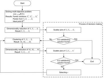
The scheme of a decision making process, using the proposed strategy is presented in Figure 2. The visualization tool is useful for a decision maker in search of the satisfactory solution. The decision maker can use some ways to evaluate the Pareto solutions. It helps to select the most preferable (satisfactory) solution.
Figure 2. The scheme of a decision making process using the proposed visualization strategy
In the strategy proposed here, it is necessary to select methods for multidimensional data clustering and visualization, based on dimensionality reduction,
as well as for searching the Pareto solutions. The k
-means method, self-organizing maps, and neural gas can be used for clustering. The principal component
precisely, when passing from multidimensional data to two-dimensional ones, and the results are comprehended and interpreted more easily as compared to that obtained by the other visualization methods, for example, parallel coordinates, Chernoff faces, Andrews curves, etc.
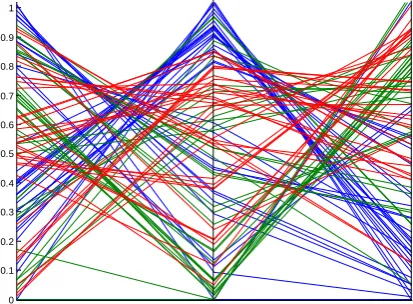
In Figure 3, the three-dimensional points
𝑌1,𝑌2, … ,𝑌100, where 𝑌𝑖=�𝑓1(𝑋𝑖∗),𝑓2(𝑋𝑖∗),𝑓3(𝑋𝑖∗)�, 𝑖= 1, … ,100, are visualized on parallel coordinates. The coordinates of the points are the values of
objectives of the Pareto front approximation, 𝑘=
100. Here the test problem DTLZ2, where 𝑚= 3 (see
Table 1), is solved. In Figure 3, a break line corresponds to a three-dimensional point. The meaning of colours is as follows: blue points mean that the Euclidian distances between them and the ideal point are the smallest ones; green points mean that the distances are average; red points mean that the distances are the largest ones. The presented results are confusing, and the interpretation is very complicated. The results, obtained by Chernoff faces and Andrews curves, are more confusing.
Figure 3. The points of the Pareto front for the problem DTLZ2 on parallel coordinates
In the experimental investigation below, we use a combination of neural gas and multidimensional scaling. Some combinations of multidimensional scaling and clustering methods, based on artificial neural networks, are proposed and investigated in [19], [20], [21]. In [19], multidimensional scaling has been combined with the self-organizing map. A comparative analysis of the combinations of multidimensional scaling with self-organizing maps and neural gas has been made in [20], [21]. The research has shown that the quantization error, obtained by the neural gas method, is smaller than that obtained by SOM. The quantization error shows how well the representatives of clusters represent all the members of the cluster.
The aim of neural gas [22] is to find a set of points
𝑀1,𝑀2, … ,𝑀𝑟 that would serve as a representation of the set of points 𝑌1,𝑌2, … ,𝑌𝑘, and the amount of the points 𝑀1,𝑀2, … ,𝑀𝑟 should be smaller than that of the points 𝑌1,𝑌2, … ,𝑌𝑘, i.e., 𝑟<𝑘, 𝑟 is selected freely.
Thus, the neural gas method can be used for data
clustering, the points 𝑀1,𝑀2, … ,𝑀𝑟 are
representatives of the clusters. The algorithm was named “neural gas” because of the dynamics of the
points 𝑀1,𝑀2, … ,𝑀𝑟 during the adaptation process
(2), which distribute themselves like gas within the data space.
𝑀𝑖(𝑡+ 1) =𝑀𝑖(𝑡) +𝐸(𝑡)ℎ𝜆(𝑖,𝑡)�𝑌𝑙− 𝑀𝑖(𝑡)�. (2)
Here 𝑌𝑙 is a point, presented to the neural gas
network; 𝑡 is the order number of iteration; 𝐸(𝑡) and
ℎ𝜆(𝑖,𝑡) are functions that control the adaptation
process [20]. At first, the initial values of 𝑀𝑖, 𝑖=
1, … ,𝑟, are selected, usually these values are random
numbers in the interval (0, 1). In each training step, a
point 𝑌𝑙∈{𝑌1,𝑌2, … ,𝑌𝑘} is presented to the neural gas
network and the points 𝑀𝑖 are changed by formula (2).
The training is continued until the maximal number of iterations is not reached. After training the points
𝑀1,𝑀2, … ,𝑀𝑟 are representatives of the points 𝑌1,𝑌2, … ,𝑌𝑘, where 𝑟<𝑘.
Multidimensional scaling (MDS) is the most popular method for multidimensional data visualization, based on dimensionality reduction [8]. The aim of multidimensional scaling is to find low-dimensional points 𝑉1,𝑉2, … ,𝑉𝑘 such that the distances
between the points in the low-dimensional space ℝ𝑠
were as close to the distances or other proximities
between the points in the multidimensional space ℝ𝑚,
as possible. Stress function (3) is minimized in it.
𝐸MDS=∑ �𝑑�𝑉𝑖,𝑉𝑗� − 𝑑�𝑌𝑖,𝑌𝑗�� 2
𝑖<𝑗 . (3)
Here 𝑑�𝑉𝑖,𝑉𝑗� is a distance between the points
𝑉1,𝑉2, … ,𝑉𝑘 in the low-dimensional space, 𝑑�𝑌𝑖,𝑌𝑗� is
a distance (or other proximity) between the points
𝑌1,𝑌2, … ,𝑌𝑘 in the multidimensional space. Usually,
the Euclidean distance is used. There are many algorithms for minimizing stress function (3). In the investigation of the paper, we use the SMACOF (Scaling by MAjorizing a Convex Function) algorithm [8]. Multidimensional scaling differs from the other popular dimensionality reduction method – the principal component analysis (PCA) – by the fact that PCA tries to preserve variances of data, while MDS tries to preserve distances (or other proximities) passing from the multidimensional space to the lower
dimensional space. In the case when 𝑚= 1, we deal
with unidimensional scaling.
4. Visualization results
Two multi-objective problems are used in the experimental investigation (Table 1) [24], [25]. These problems are commonly used for testing multi-objective optimization algorithms. In this paper, the problems are used in order to demonstrate the visualization strategy, proposed in Section 3. The
problem ZDT1 is bi-objective (𝑚= 2). The number 𝑛
of variables is freely selected. So, the problem is used in this investigation to observe that visualization by multidimensional scaling preserves the neighbourhood
of the points where the two-dimensional space ℝ2 is
changed to the one-dimensional space ℝ1.
The number of objectives as well as that of variables of the problem DTLZ2 is freely selected, too. The problem allows us to demonstrate the visualization strategy proposed, when visualizing the
Pareto front points the dimensionality of which is more than three.
The points of the Pareto front approximation are obtained by NSGA-II. As mentioned above, only an approximation of the Pareto front, but not the exact front is found by NSGA-II. The goal of this investigation is not to find the approximation as accurate as possible, but to demonstrate the visualization of the Pareto front (or approximation).
Table 1. Multi-objective optimization problems
Name Objectives Properties
ZDT1 𝑔= 1 + 9∑𝑛𝑖=2𝑥𝑖⁄(𝑛 −1), 𝑓1=𝑥1,
𝑓2=𝑔�1− �𝑓1⁄ �𝑔 .
𝑚= 2, 𝑛 is freely selected, 𝑥𝑖∈[0, 1]; Pareto front is formed with 𝑔(𝑋) = 1.
DTLZ2 The set of variables {𝑥1, … ,𝑥𝑛} =�𝑥1, … ,𝑥𝑗,𝑥𝑗+1, … ,𝑥𝑛� is divided into two distinct sets �𝑦1, … ,𝑦𝑗� and �𝑧1, … ,𝑧𝑝� as follows: �𝑦1, … ,𝑦𝑗�=�𝑥1, … ,𝑥𝑗�,
�𝑧1, … ,𝑧𝑝�=�𝑥𝑗+1, … ,𝑥𝑛�.
𝑔=∑𝑝𝑖=1(𝑧𝑖−0.5)2,
𝑓1= (1 +𝑔)∏𝑚−1𝑖=1 cos �𝑦𝑖2𝜋�,
𝑓𝑟=2:𝑚−1= (1 +𝑔)�∏𝑖=1𝑚−𝑟cos �𝑦2𝑖𝜋��sin�𝑦𝑚−𝑟+12 𝜋�,
𝑓𝑚= (1 +𝑔)sin�𝑦12𝜋�.
𝑚 and 𝑛 are freely selected; 𝑝=𝑛 − 𝑚+ 1; 𝑥𝑖∈[0, 1]. Pareto solutions 𝑥𝑖∗= 0.5, if 𝑥𝑖∗∈
{𝑧1, … ,𝑧𝑝} and all objectives satisfy: ∑ �𝑓𝑚𝑗=1 𝑗∗�2= 1.
Since the problem ZDT1 has only two objectives, the points of the Pareto front can be presented as a
scatter plot (Figure 4). Here 𝑛= 6, the size of
population (𝑝𝑝𝑝) is equal to 20, the number of
generations (𝑔𝑔𝑛) is equal to 200, when running
NSGA-II. The Euclidean distances between the Pareto
front points and the ideal point (0, 0) are computed
and the points are coloured according to the distances. Blue points mean that the distances between them and the ideal point are the smallest ones; green points mean that the distances are average; red points mean that the distances are the largest ones. The same meaning of colours remains in the figures below.
Figure 4. The points of the Pareto front for the problem ZDT1
The two-dimensional points from Figure 4 are mapped onto a one-dimensional space (a line) by unidimensional scaling. The results obtained are presented in Figure 5. We can see that the distances between the neighbouring points are preserved when passing from the two-dimensional space into the one-dimensional one. It means that the reduction of dimensionality does not distort the data.
The points from Figure 4 are clustered by the neural gas method, and representatives of the clusters are visualized by unidimensional scaling (UDS). The results obtained are presented in Figure 6. We can see that the nearest points in Figures 4 and 5 are represented as a point in Figure 6. Here, the aim of clustering is reduction of the number of solutions, which should be evaluated by a decision maker. In this
case, the number of solutions decreases from 20 to 10.
Figure 5. The points of the Pareto front for the problem ZDT1 mapped by UDS onto a line
Figure 6. The points of the Pareto front for the problem ZDT1 mapped by neural gas and UDS onto a line
0 0.2 0.4 0.6 0.8 1
0 0.2 0.4 0.6 0.8 1 1.2
11 6 9
8 3 5
7
4 15 12
14
17 18
19 13 16
20 1 10
2
f1
f2 131919 17 15 4 3 8 6 11 9 5 7 12 1418
16 20
1
10 2
3,6,8 9,11 5,7
17 4,15 12,14
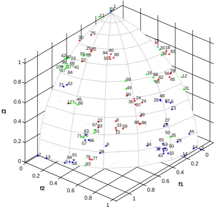
When solving the problem DTLZ2 (𝑚= 3, 𝑛= 8,
𝑝𝑝𝑝= 100, 𝑔𝑔𝑛= 200), the Pareto front points are presented in a 3D plot in Figure 7. The points are distributed in a quarter of the sphere. The number of
points is equal to 100, 𝑘= 100. Multidimensional
scaling is applied to the three-dimensional points, the two-dimensional points are obtained and they are presented in a scatter plot (Figure 8). We can see that the points are distributed in a triangular area. Moreover, the neighbourhood of the points is preserved, i.e., the close points of Figure 7 also remain close in Figure 8.
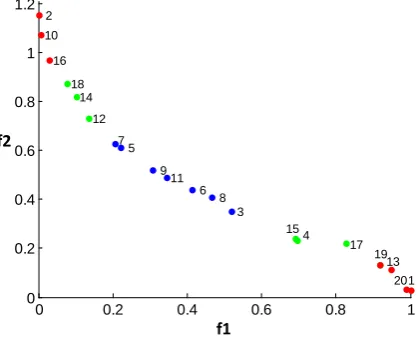
In Figure 9, the results of a combination of neural gas and MDS are presented. We can see that the nearest points (cluster) of Figure 8 are represented as a point in Figure 9. In this case, the number of the points visualized decreases from 100 to 47. The decision maker has to evaluate about two times less points than in the previous case. So, the smaller the
value of 𝑟 is selected, the smaller the number of points
(solutions) is presented for a decision maker. The
decision maker can select various values of 𝑟, and
observe the results obtained (see Figure 2).
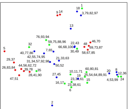
When solving the problem DTLZ2 (𝑛= 12,
𝑝𝑝𝑝= 100, 𝑔𝑔𝑛= 200), in case of the number of
objectives 𝑚 being equal to 4, a direct visualization of
the Pareto front is impossible. The dimensionality is reduced from 4 to 2 by multidimensional scaling, and the two-dimensional points are represented in a scatter plot (Figure 10). In Figure 11, the results of a combination of neural gas and MDS are presented. Some clusters of the points are obtained.
The visualization strategy proposed can be applied in visualizing the Pareto front points when the number of objectives is larger. Moreover, a decision maker gets information about distances of the solutions from the ideal point.
Figure 7. The points of the Pareto front for the problem DTLZ2 (𝑚= 3)
Figure 8. The points of the Pareto front for the problem DTLZ2 (𝑚= 3) mapped by MDS onto a plane
Figure 9. The points of the Pareto front for the problem DTLZ2 (𝑚= 3) mapped by neural gas and MDS onto a
plane
Figure 10. The points of the Pareto front for the problem DTLZ2 (𝑚= 4) mapped by MDS onto a plane 0 0.2 0.4 0.6 0.8 1 0 0.2 0.4 0.6 0.8 1 0 0.2 0.4 0.6 0.8 1 3 54 44 31 14 12 f1 29 73 81 45 78 35 6 60 10 18 92 27 56 50 19 53 79 38 48 65 20 82 43 32 72 26 95 98 34 16 86 74 39 24 97 88 36 90 49 69 59 33 15 9 80 4 1 40 8 55 94 28 11 83 22 51 77 85 67 75 96 25 76 89 93 63 70 57 52 91 30 66 71 46 41 58 61 7 23 68 62 17 64 84 37 87 5 99 42 21 47 100 13 f2 2 f3 2 13 4 44 79 53 60 54 65 10 32 3 62 8 28 26 48 27 21 43 19 14 61 64 34 29 5 92 73 58 6 63 96 57 70 71
38 11
1
20
42
37
84 68
23 87 16 93 98 95 35 50 47 41 31 51 99 66 46 67 91 69
49 89
Figure 11. The points of the Pareto front for the problem DTLZ2 (𝑚= 4) mapped by neural gas and MDS onto a
plane
5. Conclusions
The necessity of visualizing the Pareto front points arises when the number of objectives is larger than two or three, and the number of Pareto solutions is rather large. If only numerical values of the Pareto front points are presented to a decision maker, it is difficult to review the whole set of points. Especially the genetic algorithms, commonly used for solving multi-objective optimization problems, generate many solutions. Reviewing and evaluating all the solutions is time consuming for a decision maker. In order to decrease the work time, a new strategy for visualizing the points of the Pareto fronts is proposed in this paper. The strategy is based on three items: clustering multidimensional points of the Pareto front; visuali-zing the points based on dimensionality reduction; marking the points according to the Euclidean distances from the ideal point. The examples with some multi-objective optimization problems have shown that the structures of Pareto fronts are preserved when passing from a multidimensional space to a low-dimensional one. In the investigation, multidimensional scaling is used as a method for dimensionality reduction, and neural gas is applied in clustering. However, the other similar methods can be used without changing the strategy proposed.
The visualization strategy proposed should be implemented in a decision support system. It would assist a decision maker to select interactively the most preferable solutions from a huge set of Pareto solutions. A combination of the genetic algorithm with visualization of the Pareto front points, based on dimensionality reduction and clustering of points, allows a decision maker to see the generalized information on the Pareto fronts. An assumption is made that there are similar solutions in a cluster. After the review of some solutions from the cluster, a decision maker can have his/her opinion about the whole cluster. Genetic algorithms usually generate a
lot of solutions, so the time for reviewing the solutions will be saved, if the decision maker searches the most preferable ones. The decision support system should have possibilities to choose the number of points of the Pareto fronts as well as the number of clusters.
Acknowledgments
One of the authors (Ernestas Filatovas) is supported by the postdoctoral fellowship is being funded by European Union Structural Funds project ”Postdoctoral Fellowship Implementation in Lithuania”.
References
[1] J. Branke, K. Deb, K. Miettinen, R. Slowiński. Multiobjective optimization. Interactive and Evolutionary Approaches. Lecture Notes in Computer Science. Springer, 2008.
[2] P. M. Pardalos, I. Steponavičė, A. Žilinskas. Pareto set approximation by the method of adjustable weights and successive lexicographic goal programming.
Optimization Letters, 2012, Vol. 6, No. 4, 665–678. [3] M. Ehrgott. Multicriteria optimization. 2nd ed.
Springer, 2005.
[4] T. Petkus, E. Filatovas, O. Kurasova. Investigation of human factors while solving multiple criteria optimization problems in computer network.
Technological and Economic Development of Economy, 2009, Vol. 15, No. 3, 464–479.
[5] E. Filatovas, O. Kurasova. A decision support system for solving multiple criteria optimization problems.
Informatics in Education, 2011, Vol. 10, No. 2, 213−224.
[6] K. Deb, S. Agrawal, A. Pratap, T. Meyarivan. A fast elitist non-dominated sorting genetic algorithm for multi-objective optimisation: NSGA-II. In:
Proceedings of the 6th International Conference on Parallel Problem Solving from Nature. London, UK: Springer-Verlag, 2000, pp. 849–858.
[7] G. Dzemyda, O. Kurasova, J. Žilinskas.
Multidimensional Data Visualization: Methods and Applications. Springer-Verlag, 2013.
[8] I. Borg, P. J. F. Groenen. Modern Multidimensional Scaling: Theory and Applications (2nd ed.), Vol. 35. Springer, 2005.
[9] A. Inselberg. The plane with parallel coordinates.
Visual Computer, 1985, Vol. 1, No. 2, 69–91.
[10] T. Kohonen. Self-Organizing Maps (3rd ed.). Vol. 30. Springer-Verlag, 2001.
[11] M. C. Ortiz, L. A. Sarabia, M. S. Sánchez, D. Arroyo. Improving the visualization of the Pareto-optimal front for the multi-response optimization of chromatographic determinations. Analytica Chimica Acta, 2011, Vol. 687, 129–136.
[12] S. Obayashi, D. Sasaki. Visualization and data mining of Pareto solutions using self-organizing map. In:
Proceedings of the Second International Conference on Evolutionary Multi-Criterion Optimization (EMO 2003), 2003, Springer-Verlag, pp. 796–809.
[13] M. Yoshimi, T. Kuhara, K. Nishimoto, M. Miki, T. Hiroyasu. Visualization of Pareto solutions by spherical self-organizing map and its acceleration on a 40,77,86
42,55,74,95 31,34,57,92,98
2 7,65
50,52
27,45 21,33,63
13
23,38,61 66,68,100
22,43 18
19 3,79,82,97
20 12,36 8 32
35 76,93,94
59,75,88,96
16,17 10,11,71
6 23,38,61
30,49 1
25,54,64,89,91 60,80,81
15 4,53,9924
5
29,37
26,83,84
47,51 44,56,62,72
39,78
28,41,90
9 14
48
58,67,85 69,73,87
GPU. Journal of Software Engineering and Applications, 2012, Vol. 5, 129–137.
[14] X. Blasco, J. M. Herrero, J. Sanchis, M. Martínez. A new graphical visualization of n-dimensional Pareto front for decision-making in multiobjective optimization. Information Sciences, 2008, Vol. 178, 3908–3924.
[15] G. Agrawal, K. Lewis, K. Chugh, C. H. Huang, S. Parashar, C. L. Bloebaum. Intuitive Visualization of Pareto frontier for multi-objective optimization in n-dimensional performance space. In: 10th AIAA/ISSMO Multidisciplinary Analysis and Optimization Conference, 2004.
[16] M. Koppen, K. Yoshida. Visualization of Pareto-sets in evolutionary multi-objective optimization. In: 7th International Conference on Hybrid Intelligent Systems, 2007, pp. 156–161.
[17] V. Lotov, V. Bushenkov, G. Kamenev. Interactive Decision Maps. Approximation and Visualization of the Pareto Frontier. Kluwer, Boston, 2004.
[18] A. V. Lotov, K. Miettinen. Visualizing the Pareto frontier. Multiobjective optimization, interactive and evolutionary approaches [outcome of Dagstuhl seminars]. Lecture Notes in Computer Science. Springer-Verlag, 2008, pp. 213–243.
[19] J. Bernatavičienė, G. Dzemyda, O. Kurasova, V. Marcinkevičius. Optimal decisions in combining
the SOM with nonlinear projection methods. European Journal of Operational Research, 2006, Vol. 173, No. 3, 729–745.
[20] O. Kurasova, A. Molytė. Integration of the self-organizing map and neural gas with multidimensional scaling. Information Technology and Control, 2011, Vol. 40, No. 1, 12–20.
[21] O. Kurasova, A. Molytė. Quality of quantization and visualization of vectors obtained by neural gas and self-organizing map. Informatica, 2011, Vol. 22, No. 1, 115–134.
[22] T. Martinetz, K. Schulten. A neural-gas network learns topologies. Artificial Neural Networks, 1991, Vol. 1, 397–402.
[23] G. Palubeckis. An improved exact algorithm for least-squares unidimensional scaling. Journal of Applied Mathematics, 2013, Vol. 2013, Article Number 890589.
[24] E. Zitzler, K. Deb, L. Thiele. Comparison of multiobjective evolutionary algorithms: Empirical results. Evolutionary Computation, 2000, Vol. 8, No. 2, 173–195.
[25] K. Deb, L. Thiele, M. Laumanns, E. Zitzler. Scalable multi-objective optimization test problems. In: Proceedings of the 2002 Congress on Evolutionary Computation, 2002, Vol. 1, pp. 825–830.