Optimising Performance and Cost at the Early Design Stages
Mohammad Saravi
*, Linda Newnes, Tony Mileham
Department of Mechanical Engineering, University of Bath, Bath, UK.
Received 25 April 2013; received in revised form 28 May 2013; accepted 24 June 2013
Abstract
When designers start to design a product, deriving a useful cost estimate at the early design stage is challenging.
This is because the available data is limited and designers need to deal with variation, especially for new products
where product specifications are often expressed as a range of values. Despite this difficulty, cost estimation should
be carried out as early as possible since, up to 80% of a product’s cost is said to have been committed in the early
design stages. One of the challenges faced is how one can optimise performance and cost. The research presented in
this paper offers a solution to this challenge. The solution is used to reduce variation in the product specification in
order to improve the quality of the cost estimate in the early design stages. The step-by-step process enables designers
to undertake an informed optimisation between performance and cost to aid in the selection of the final concept. To
achieve this, the research presented in this paper proposes the use of Taguchi’s orthogonal array approach to reduce
variation in the product specification. Within this paper, a critique of the literature and industrial context is offered,
demonstrating the need for such an approach. From this critique, the research question ‘How can we improve the
quality of the average cost during the early design stages using the limited information available? It defined and novel
process is described. Finally, a pilot and industrial case study are used to demonstrate how the process would be used.
The outcome illustrates how designers can use this process to estimate the lowest possible average cost with the
lowest variance.
Keywords: cost estimation, Taguchi’s orthogonal array approach, concept development process
1.
Introduction
Companies need to know the estimated cost of a product and the confidence of that estimate in order to design and
manufacture a product in detail [1]. Having reliable and robust cost estimate for future product enables designers to focus their
time on suitable designs/products and reduces the designers spending their tome and money on designing non-economical
products. To reduce this none-value adding time there is a need to estimate the cost of the products as early as possible within
the design process. Hence, enabling informed decisions on the concept(s) to be investigated further. However, when one
evaluates the current approaches used in cost estimation, existing techniques appeared to be increasingly prone to error, with
mistakes being many and varied. An example is the Airbus A380 where the actual costs differ from those predicted [2]. Roy et
al. [3] identify that there are many risks associated with not costing a project properly. Many authors such as Wasim et al. [4]
and Houseman et al. [5] have indicated that both underestimates and overestimates can have negative impacts on a company’s
business. Asiedu and Gu [6] state that “the greater the underestimate, the greater the actual expenditure”, the greater the
overestimate, the greater the expenditure” and “the most realistic estimate results in the most economical project cost”. Fig. 1,
often referred to as the Freiman curve depicts these claims.
Fig. 1 The Freiman curve
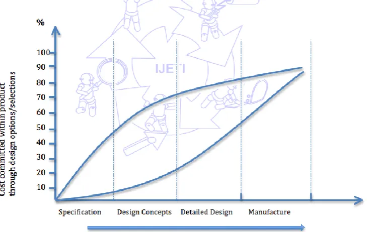
Although there are many researchers have pointed out the importance of cost estimation at the early design stages, where
it is often claimed that up to 80% of the costs are built into the product [7-9]. However, estimating cost at the conceptual stage
of design is often difficult since available information is limited and designers need to wait until more detail and information is
available. Fig. 2 illustrates that high percentage of products costs are determined at the conceptual stage of design.
Fig. 2 Cost commitment during design
Although there are different definitions of design, it can be broken into three major stages: Conceptual design,
Embodiment design and Detail design [10]. Conceptual design is considered to be the most important stage in terms of
decision-making in design. It is during conceptual design that the basic questions of configuration arrangement size, weight and
performance are answered [11]. In the Embodiment and Detail design stages, materials, specifications, dimensions, surface
As stated previously up to 80% of the products costs are determined at the conceptual stage of design, the focus of this
research is based on available information at this stage of product design. The concept design stage has a number of steps.
Ulrich and Eppinger [12] have identified seven major stages: 1. Identify customer needs, 2. Target specifications, 3. Generate
product concepts, 4. Select product concepts, 5. Test product concepts, 6. Set final specifications and 7. Plan downstream
specifications.
Normally designers do not consider the ‘identify customer needs’ stage as part of the conceptual design process. Ulrich
and Eppinger however emphasize the importance of this stage before the concept development process begins to ensure the
needs are fully understood. The next stage is to set the target specification for use in the first stage in the conceptual design
process. It is at this stage that agreement on the general design functions is achieved, with the target specifications being set to
meet the design requirements. However, they are established before the designers know what constraints the product technology
will place on the design and what can be achieved [12]. Hence, targets are expressed as a range of values, such as shown in Table
2.
For the target specification the values are wide and are reduced throughout the designs stages accumulating in the final
specification list. Because of these wide values in the initial product specification, estimating costs is often a challenge. As these
values are the only available information at the beginning of the conceptual design, the focus of this research is based on using
the target specification (using the metrics values) to improve the quality of the average cost at the conceptual stage of design.
To estimate the cost of a product, different techniques are often used. This is due to the available information being
different at the various stages of product design and development. Xiachuan et al. [13] classify cost estimation techniques into
five main cost estimation methods: parametric, analogy, artificial neural network (ANN), activity-based costing (ABC) and the
engineering cost method. Table 1 summarises their definition of precision and uncertainty of cost estimation techniques at
different stages of the design process. As parametric estimation techniques are one of the most popular and useful techniques
used by designers at the conceptual stage of design, this technique was selected for use in the research using SEER-DFM
commercial cost estimation software.
Table 1 Precision of cost estimation methods.
Cost estimation methods
Properties
Uncertainty Phase of design process Precision
Parametrics Low Early Middle
Analogy High Late Middle
ANN Middle Early High
ABC High Late High
Engineering Low Late High
2.
Research Question and Proposed Process
The research question was ‘How can we improve the quality of the average cost during the early design stages using the
limited information available?’ To answer this question, a novel process is introduced in this paper. The proposed process
consists of three phases as depicted in Fig. 3. The first phase consists of analyzing the product specification. Phase 2 is
estimating the manufacturing cost and variance of the cost estimate. The final phase is the final concept selection. Each of these
phases is described in detail in the next section. To illustrate the process, a pilot case study is used to illustrate how phases 1 and
2 are performed via a product demonstrator. Phase 3, selecting the final concept, uses an industrial case study is used to validate
Fig. 3 Performance and Cost optimisation process
3.
Pilot Case Study: Fluid Dispenser for Elderly People (Phase 1 & 2 of the Proposed Process)
This case study was based on the concept design of a novel fluid dispenser for people who are not able to use conventional
cups. The requirements were translated into engineering terms and a target specification created, provided in Table 2. The
designer identified eleven metrics of factors (1 – 11) and these target specification metrics were then rated in terms of their
functionality, using Quality Function Deployment (QFD) techniques [14].
Table 2 The target specification for fluid dispenser [15]
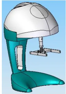
Four concept designs were created based on; a plunger-based, disposable cup, armband, and camelback, using the defined
target specification (Table 2). The following sections illustrate a step-by-step implementation of the process for the
processes were used to manufacture it, it was selected as an example in this paper). Table 3 lists, the sub-components or parts
used in the plunger-based concept and their quantity. The drink dispenser was designed for a production quantity of 7000 units.
Fig. 4 The plunger based concept
Table 3 The plunger-based sub-components and their quantities
3.1. Phase 1 – Analysing Product Specification
(1) Identifying factors which are thought to have the greatest impact on product cost.
The first stage was to identify factors which were considered to have the greatest impact on the cost of the plunger-based
concept. For products with only a few factors there is no need to identify cost factors. This is because all the factors can be
assessed as it is not time consuming. As for the fluid dispenser project, eleven factors identified: the Delphi method [16] factors,
which were thought to have the greatest impact on the fluid dispenser cost.
To do this, more than 16 experts in engineering design and cost estimation were interviewed. Two questionnaires were
designed and then completed by the experts, and the results were analysed. This resulted in seven cost factors (A, B, E, F, G, H
and I) being identified, shown in Table 4. Along with the seven cost factors, five interactions (AxG, GxH, IxG, GxB and AxB)
were also identified for examination (the interaction between Factor A and B is presented as AxB).
(2) Identifying factor levels
After identifying the factors, the next stage was to identify factor levels. Levels identified for the selected factors are
shown in Table 4 (in this paper a level means possible values from the product specification for each factor). As shown, two
levels were identified for each factor (more than two levels can be examined if greater accuracy is required). For example, for
factor A (total mass when full), 3 kg was selected for level 1 and 3.5 kg for level 2. Appropriate levels were similarly selected for
all other factors. All of the levels selected were within the target specification.
3.2. Estimating Manufacturing Cost and Variance of Cost Estimate (1) Selecting an appropriate orthogonal array
The first stage in this phase was to select the most appropriate orthogonal array and assign factor levels to the orthogonal
array. Xiachuan et al. [13] describe in detail how to select the most appropriate orthogonal array. As described in the previous
section, seven factors (A, B, E, F, G, H and I) and five interactions (AxG, GxH, IxG, GxB and AxB) were identified. Since
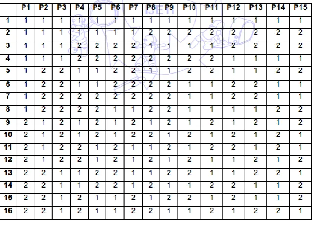
seven factors and five interactions needed to be examined, the most appropriate orthogonal array was an L16(215). Table 5
shows an example of the standard L16(215) orthogonal array introduced by Taguchi.
Table 5 The standard L16(215) orthogonal array
(2) Assigning factors and factor levels to the selected orthogonal array
After selecting the most appropriate orthogonal array, the next step was to assign the factors and interactions to it. To
assign the factors (seven factors and five interactions), the linear graph was used. Linear graphs help designers to assign factors
and interactions to an orthogonal array by presenting factor and interaction assignments in diagrammatic form. In other words,
designers can use the linear graph to more easily assign factors to an orthogonal array (how to use the linear graph is explained
First the factors and any relationships between them (interaction) was analysed (dots represent factors and the lines
represent the interaction between factors). After analysing the relationship between factors the next step was to use the linear
graph and assign the factors to the L16 (215) orthogonal array. Fig. 5(a) shows the standard linear graph for L16. The required
linear graph was then matched to the standard linear graph. Fig. 5(b) illustrates the required linear graph for the plunger-based
concept.
Fig. 5 The standard and required linear graph (L16) for the plunger-based concept
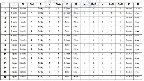
The next step was to assign the factors (seven factors and five interactions, in total 12 factors) to the standard L16(215)
orthogonal array (Table 5). Using Fig 5 and Table 5, factors were assigned to the L16(215) orthogonal array as is shown in
Table 6. The selected factors were assigned to the L16(215) orthogonal array namely; (I→P1, G→P2, GxI→P3, A→P4, e→P5,
GxA→P6, F→P7, B→P8, e→P9, GxB→P10, e→P11, AxB→P12, GxH→P13, E→P14 and H→P15) with the empty columns being denoted as ‘e’ representing an error. For this research the ‘e’ indicates columns that do not have any real effect on the
result.
After assigning the factors, the next stage was to assign factor levels. Using Table 5, factor levels for the plunger-based
concept were assigned as shown in Table 6. Since exp 1 to exp 8 (Table 5) should be level one, level one for factor I (8 parts)
was assigned to Exp 1 to Exp 8. Also as exp 9 to exp 16 (Table 5) should be level two, level two for factor I (10 parts) was
assigned to exp 9 to exp 16. Appropriate levels were similarly added for all the other factors. Table 6 shows the completed L16
(215) orthogonal array for the plunger-based concept after assigning factors and their levels. It is important to note that the same
table could be used for other concepts but at this stage it is shown for the plunger-based concept to depict the case study.
(3) Estimating manufacturing cost for each concept
Here, the manufacturing cost of the plunger-based concept for each experiment was calculated and inserted into Table 6.
Using Table 6, sixteen experiments were carried out and the manufacturing cost of the plunger concept for each experiment was
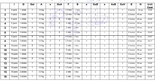
estimated using the SEER-DFM software. The estimated values were then placed in the last column to create Table 7. Table 7
illustrates the L16 (215) orthogonal array for the plunger-based concept after adding the estimated cost for each experiment.
Using experiment 1 as an example, the cost of the plunger concept was 19.91 cost units for the combination of factors. In other
words, for the plunger-based concept design (Fig. 4), if factor I was 8 parts, factor G was 1 drink, factor A was 3.0kg, factor F
was 1.5min, factor B was 1litre, factor E was 1 action and factor H was 20sec, the manufacturing cost of the plunger concept was
19.91 cost units. The costs of the other experiments were similarly calculated. As shown in Table 7, the smallest cost of the 16
experiments for the plunger concept was 19.09 cost units and the highest cost was 24.93 cost units. A SEER-DFM file was
created for each experiment for the plunger-based concept.
Table 7 Orthogonal array and unit costs for the plunger-based concept
(4) Calculating the average and variance of manufacturing cost of concept
To calculate the average and variance of the manufacturing cost for, the plunger-based concept was calculated by using
the unit cost of experiment 1 to experiment 16, as shown in Table 7. The average manufacturing cost for the plunger concept was
(this is called the average manufacturing cost before optimisation).
The average manufacturing cost for the plunger-based concept was:
Y = n
Where:
y1 is cost of experiment 1
yn is cost of experiment n
n is number of experiments
Therefore, from (1)
19.91 + … + 24.32
Y = = 22.70 cost units 16
The variance of the manufacturing cost for the plunger-based concept was:
Σy² - nY² (y12 + ... + yn2) – (Y)2 σ² n-1 = = n – 1 n - 1
(2)
Where;
Y is the average manufacturing cost (from Eq. (1))
y1 is cost of experiment 1
yn is cost of experiment n
n is number of experiments
Therefore, from (2)
(19.912 + ... + 24.322) – (22.70)2
σ² n-1 = = 3.95 cost units 16 - 1
In summary the results showed that the:
Average cost before optimisation: 22.70 cost units
Variance of the cost estimates before optimisation: (σ²): 3.95 cost unit
(5) Identifying optimum solution
As previously stated, the main aim of this research was to estimate the lowest possible manufacturing cost and the lowest
possible variance of manufacturing cost that designers could achieve by selecting the most appropriate factor levels for the
design (whilst meeting the specifications). To reduce the variance of the manufacturing cost for the plunger concept, the effect
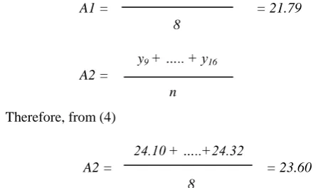
of different levels for each factor were compared. For example, the effect of I1 (level one of factor I) and I2 (level two of factor
I) were compared by taking the average of estimates in those experiments using I1 (experiment numbers 1, 2, 3, 4, 5, 6, 7 and 8)
with the average for experiments using I2 (9-15, 16) shown in Table 7. Using Table 7, the average effect of both level one and
level two for factor I for the plunger concept were:
y1 + ….. + y8
A1 = n
(3)
Therefore, from (3)
A1 = = 21.79 8
y9 + ….. + y16
A2 = n
(4)
Therefore, from (4)
24.10 + …..+24.32
A2 = = 23.60 8
The effect of level one and two for other factors were similarly calculated. These results were then added to the response
table, shown in Table 8. Here, the difference between level 1 and level 2 for each factor was calculated and factors with the
highest difference ranked as factors that had the greatest impact on the uncertainty of the cost estimate for the plunger concept.
As shown in Table 8, factor G had the greatest impact and factor AxB had the smallest impact on the uncertainty of the cost
estimate.
Table 8 The response table for the plunger-based concept
The next stage was to select the most appropriate level for each factor to reduce the variance of the manufacturing cost. As
a rule of thumb [13]), half of the factors (G, I, E, F and GxI) i.e. those which had the greatest impact on the uncertainty of the
cost estimate for the plunger concept should be selected for further analysis. But when an interaction is amongst the selected
factors for a product, it does not mean that it can be selected for further analysis. First the response graph should be created to
check if there is an interaction.
In the case of the plunger-based concept, interaction GxI (it was among the factors which had the greatest impact on the
uncertainty of the cost estimate) was examined to check if there was an interaction between factors G and I. To check if there
was an interaction between factor G and I, the effect of level 1 and level 2 for factor GxI were calculated. Using table 7, the
average effect of both level one and level two for factor GxI for the plunger concept were:
G1xI1 = (19.91 + 19.09 + 22.02 + 22.75)/4 = 20.94 cost units
G1xI2 = (24.1 + 23.27 + 20.56 + 21.29)/4 = 22.30 cost units
G2xI1 = (21.52 + 22.06 + 24.87 + 22.17)/4 = 22.65 cost units
G2xI2 = (24.92 + 25.47 + 24.93 + 24.32)/4 = 24.96 cost units
The effect of level 1 and level 2 of factor GxI are shown in Fig. 6. As shown, there was no interaction between factor G
and I (since the interaction breakdown was parallel) for plunger-based concept. Therefore, GxI was not considered as one of the
selected factors (G, I, E and F) for further analysis.
To reduce the uncertainty, one level for each of the selected factors (G, I, E and F) were chosen (levels for the selected
“smaller-the-better” was used as the output. Therefore, from the results shown in Fig. 6, the most appropriate factor levels to
reduce cost could be I1, G1, F1 and E2 (they appear to lead to the lower cost for the plunger concept). However, as lower cost
does not necessarily mean better performance a trade-off between performance and cost was carried out. In case of factors I, G
and F, since they were rated only 3 in terms of performance (Table 4), it can be assumed that choosing the lowest cost level will
have minimum effect on the performance. Therefore I1, G1 and F1 were selected as the most appropriate levels. But in the case
of factor E, since factor E was rated 5 in terms of performance (shown in Table 4), any trade-off should be considered carefully.
Although selecting E2 could generate a lower cost, E1 was selected to maximize the performance requirement. In a real
situation the designer would have all the information to make a rational trade-off decision. Therefore the optimum solution for
the plunger concept was I1 (8 parts), G1 (1 drink), F1 (1.5 min) and E1 (1 action).
Fig. 6 Factor/Levels
(6) Calculating the average cost and variance of manufacturing cost after optimisation
After carrying out the initial optimisation and trade-off, the only factors with a choice of levels were A, B and H as the
levels for I, G, F and E were now fixed. It is important to notice that the reason for adding interactions to Table 8 in the previous
section was to check if there was any interaction between factors. As just one interaction (GxI) was among the selected factors
which had the greatest impact on the product manufacturing cost, this interaction was examined. Reviewing Fig. 6, there is no
interaction between factors G and I as they are roughly in parallel with one another. Therefore, none of the interactions (GxI,
GxA, GxB, AxB and GxH, shown in Table 8) were selected for further analysis. The next step was to select the most
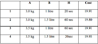
appropriate orthogonal array for the remainder of the factors (A, B and H). Since three factors in two levels (level one and two)
needed to be examined, the standard L4(23) orthogonal array was selected and the manufacturing cost of the plunger concept for
each experiment was calculated, as shown in Table 9.
After adding the estimated cost to Table 9, the next and last stage of phase 2 of the proposed process was to calculate the
average and variance of manufacturing cost of the plunger concept after optimisation. The average manufacturing cost for the
plunger concept after optimisation was:
Y = (19.91 + 19.80 + 19.91 + 19.93)/4 = 19.88 cost units
The variance of the manufacturing cost for the plunger-based concept was:
Σy² - nY²
σ² n-1 = = 0.40 cost units n - 1
In summary the results after optimisation were:
(a) Average cost after optimisation: 19.88 cost units.
(b) Variance of cost estimate (σ²): 0.40 cost units.
Table 10 shows the average and variance of the manufacturing cost for the plunger concept before and after optimisation.
It illustrates that the average manufacturing cost before optimization was 22.70 cost units and after optimization the average
manufacturing cost had reduced to 19.88 cost units. Also the variance of the manufacturing cost for the plunger concept was
reduced from 3.95 to 0.40 cost units. The optimum solution showed the lowest possible cost and the lowest possible variance of
the cost that the designer could achieve by selecting appropriate factor levels for the plunger concept (whilst meeting the
specifications).
Table 10 The average and variance of manufacturing cost for the plunger-based concept before and after optimisation
It is important to notice that the variance of the manufacturing cost for the plunger-based concept was reduced because the
most appropriate values (levels) for factors/metrics I, G and F (factors which had the greatest impact on the product cost, Table
4) were selected and fixed. The variance of the manufacturing cost for the plunger concept could be reduced further if further
optimisation was undertaken for the remaining factors/metrics (A, B and H) and if their values were fixed. But since the effect
of the remaining factors/metrics (A, B and H) on the product cost were low, their values have not been fixed at this stage
(expressed in ranges). This can assist the designers to have more options in the next stage of design (embodiment or detail) to
improve the product design.
3.3. Comparing and Selecting the Final Concept
As mentioned before, the pilot case study (the plunger-based concept was used to illustrate phase 1 and 2 of the proposed
process. Phase 3 (comparing and selecting the final concept) is explained in the following section using an industrial case study.
4.
Industrial Case Study (Proximal Jig)
To illustrate the phase 3 of the proposed process an industrial case study was undertaken. The aim of the project
undertaken in conjunction with DePuy was to design a new Proximal Tibial Jig in order to assist surgeons to cut the Tibial bone
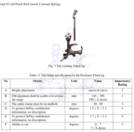
in the knee easily and accurately during knee replacement operations. Fig. 7 shows the existing Tibial jig used by surgeons. The
undertaken by designers within the DePuy. The user requirements were identified. These user requirements were then translated
into engineering terms and a target specification created as summarized in Table 11. Six metrics or factors (A, B, C, D, E and F)
were identified and these factors were expressed as a range of values. The factors in the target specification were rated in terms
of their functionality using Quality Function Deployment (QFD) techniques. Using the defined target specification, six concept
designs were created. Three of these concepts are used to illustrate the third phase of the proposed process:
(a) Concept 01 (All Dial Rack based, Live Spring).
(b) Concept 02 (Combo A Dials & Levers, Live Spring).
(c) Concept 03 (All Pinch Rack based, Constant Spring).
Fig. 7 The existing Tibial Jig
Table 11 The target specification for the Proximal Tibial jig
No Metric Unit Value Importance
Rating
A Height adjustment macro & micro 5
B EM alignment shall be usable over at least the range
mm 245 – 390
390 ≤ X desire
3
C The ankle clamp must fit on malleoli ranging in breadth
mm 50 - 90
90 ≤ X desire
3
D To protect DePuy confidential information, no description
degrees 1.5 ≤ X < 2.3 4
E To protect DePuy confidential information, no description
degrees 1.7 ≤ X < 2.3 4
F Ability to cut degrees 0 – 7
7 ≤ X desire
3
4.1. Phase 3 – Comparing and Selecting the Final Concept.
Using phase 1 and 2 of the proposed process (explained in the previous section, pilot case study), the average and
variance of manufacturing cost before and after optimisation for each of three concepts were calculated. To compare the cost
and variance of the cost for each of the concepts the results were summarized as shown in Table 12. The average cost and
variance of the cost of three concepts (01-03) were reduced after optimisation. For concepts 03, the average manufacturing cost
after optimisation was increased. This occurred as factor A had a very high impact on concept 03 in terms of the cost. As factor
A was rated 5 (Table 12) in terms of performance, A2 (micro) needed to be selected. That is why the average cost after
optimisation was increased, even though the variance of the cost of this concept was still reduced. One of the most interesting
outcomes after applying this method and comparing the results before and after optimisation (Table 12) was the results show
average cost of concept 03 (327.06) was higher than the average cost of concept 01 (325.24). This was again because factor A
had a higher impact on the cost of concept 03 compared to concept 01. This indicates the importance of applying this method
and undertaking an optimisation between performance and cost at the conceptual stage of design. Comparing results for
concepts 01, 02 and 03 after optimisation, the average manufacturing cost and variance of the manufacturing cost for concept 01
was lower than concepts 01 and 03. Therefore, concept 01 was selected as the final design by the designers.
Table 12 Comparing results before and after optimisation
Concept 01 Concept 02 Concept 03
Be fo re O p tim isa tio n Co st
330.86 345.94 323.74
Va
ria
n
ce
318.20 301.92 631.91
Afte r O p tim isa tio n co
st 325.24 340.25 327.06
Va
ria
n
ce
46.18 46.70 52.67
Afte r Fi n a l O p tim isa tio n Co st
319.38 334.39 321.20
5.
Conclusions
This paper has presented a new process to estimate the lowest possible manufacturing cost and the lowest possible
variance to help designers to select the final concept, whilst meeting the specification. The main contribution of this research is
that the new process can assist designers to rate the product specifications in terms of cost in order to carry-out more informed
trade-off between performance and cost at the early design stages. Although the new process help managers to identify factors
which have the greatest impact on product cost and hence estimate cost and variance of cost for a product, it also give them an
option to find out how changing the values in the product specifications can affect the output in terms of cost and performance.
Although the new process can be used for any mechanical products, estimating cost for products with high number of factors in
the product specifications can be time consuming. Therefore, some techniques such as Delphi method can be used to ease the
process. The proposed process presented in this research paper was based on reducing variation in the product specifications to
estimate a single point estimate for each experiment and the uncertainty in the single point is unknown. The future work is
focused on reducing the uncertainty of each single point estimate.
Acknowledgements
The article is a revised and expanded version of a paper entitled “Improving the quality of the cost estimate by enhancing
optimisation between performance and cost at the early design stages” presented at the 27th international conference on
References
[1] J. C. Farineau, B. Rabenasolo, J. M. Castelain, Y. Meyer and P. Duverlie, “Parametric models in an economic evaluation step during the design phase,” International Journal of Advanced Manufacturing Technology, vol. 12, pp. 79-86, 2011. [2] BBC, “Airbus hikes A380 break-even marks,” London, 2006.
[3] R. Roy, S. Forsberg, S. Kelvesjo and C. Rush, “Quantitative and qualitative cost estimating for engineering design,” Journal of Engineering Design, vol. 12, pp. 147-162, 2001.
[4] A. Wasim, E. Shehab, A. Al Shaab, R. Alarm, H. Abdollah and R. Sulowski, “Cost modeling system for lean product and development,” Proceeding of the 9th ed. International Conference on Manufacturing Research ICMR, 2011.
[5] O. R. Houseman, R. Rajkoumar, C. Mainwright and E. Lavdas, “Cost optimising aircraft system at a conceptual design stage,” International Journal of Manufacturing Technology and Management, vol. 15, pp. 328-345, 2008.
[6] Y. Asiedu and P. Gu, “Product Life cycle cost analysis: state of art review,” International Journal of Production Research, vol. 36, pp. 883-908, 1998.
[7] J. Corbett, “Design for Economic Manufacture,” Annals of the CIRP, vol. 35, 1986.
[8] R. Curran, S. Raghunathan and M. Price, “Review of Aerospace Engineering Cost Modelling: The Genetic Casual Approach,” Progress in Aerospace Sciences, vol. 40, pp. 487-534, 2004.
[9] L. B. Newnes, A. R. Mileham, W. M. Cheung, R. Marsh, J. D. Lanham, M. E. Saravi and R. W. Bradbery, “Predicting the
whole-life cost of a product at the conceptual design stage,” Journal of Engineering Design, vol. 19, pp. 99-112, 2008. [10] G. Pahl, W. Beitz, K. Wallace, J. Feldhusen, L. Blessing and K. H. Grote, Engineering design: a systematic approach, 3rd
ed. London Limited: Spering-Verlag, 2007.
[11] D. P. Raymer, Aircraft design: A conceptual approach, American Institute of Aeronautics and Astronautics, London, UK,
1999.
[12] K. T. Ulrich and S. D. Eppinger, Product design and development, 3rd ed. McGraw-Hill Higher Education, NY USA, 2003.
[13] C. Xiachuan, Y. Jianguo, L. Beizhi and F. Xin-an, “Methodology and technology of design for cost (DFC),” Intelligent and Automation, IEEE, vol. 3, pp. 2834-2840, 2004.
[14] J. P. Ficalora and L. Cohen, QualityFunction Deployment and Six Sigma, 2nd ed. New York: Prentice Hall, 2012. [15] C. Bennett, “A fluid dispenser for older people,” MEng Specialist Design Project Report, Dept. Mech. Eng., University of
Bath, UK, 2008.
[16] C. Chien-Hsu and A. Stanford, “The Delphi technique: making sense of consensus,” Practical assessment, Research and
evaluation, vol. 12, 2007.
![Table 2 The target specification for fluid dispenser [15]](https://thumb-us.123doks.com/thumbv2/123dok_us/9829312.1969047/4.595.212.415.61.360/table-target-specification-fluid-dispenser.webp)