Classification in Networked Data:
A Toolkit and a Univariate Case Study
Sofus A. Macskassy [email protected]
Fetch Technologies, Inc.
2041 Rosecrans Avenue, Suite 245 El Segundo, CA 90254
Foster Provost [email protected]
New York University 44 W. 4th Street New York, NY 10012
Editor: Andrew McCallum
Abstract
This paper1 is about classifying entities that are interlinked with entities for which the class is known. After surveying prior work, we present NetKit, a modular toolkit for classification in net-worked data, and a case-study of its application to netnet-worked data used in prior machine learning research. NetKit is based on a node-centric framework in which classifiers comprise a local clas-sifier, a relational clasclas-sifier, and a collective inference procedure. Various existing node-centric relational learning algorithms can be instantiated with appropriate choices for these components, and new combinations of components realize new algorithms. The case study focuses on univari-ate network classification, for which the only information used is the structure of class linkage in the network (i.e., only links and some class labels). To our knowledge, no work previously has evaluated systematically the power of class-linkage alone for classification in machine learning benchmark data sets. The results demonstrate that very simple network-classification models per-form quite well—well enough that they should be used regularly as baseline classifiers for studies of learning with networked data. The simplest method (which performs remarkably well) highlights the close correspondence between several existing methods introduced for different purposes—that is, Gaussian-field classifiers, Hopfield networks, and relational-neighbor classifiers. The case study also shows that there are two sets of techniques that are preferable in different situations, namely when few versus many labels are known initially. We also demonstrate that link selection plays an important role similar to traditional feature selection.
Keywords: relational learning, network learning, collective inference, collective classification, networked data, probabilistic relational models, network analysis, network data
1. Introduction
Networked data contain interconnected entities for which inferences are to be made. For example,
web pages are interconnected by hyperlinks, research papers are connected by citations, telephone accounts are linked by calls, possible terrorists are linked by communications. This paper is about
within-network classification: entities for which the class is known are linked to entities for which
the class must be estimated. For example, telephone accounts previously determined to be fraudu-lent may be linked, perhaps indirectly, to those for which no assessment yet has been made.
Such networked data present both complications and opportunities for classification and ma-chine learning. The data are patently not independent and identically distributed, which introduces bias to learning and inference procedures (Jensen and Neville, 2002b). The usual careful separation of data into training and test sets is difficult, and more importantly, thinking in terms of separating training and test sets obscures an important facet of the data: entities with known classifications can serve two roles. They act first as training data and subsequently as background knowledge during inference. Relatedly, within-network inference allows models to use specific node identifiers to aid inference (see Section 3.5.3).
Networked data allow collective inference, meaning that various interrelated values can be in-ferred simultaneously. For example, inference in Markov random fields (MRFs, Dobrushin, 1968; Besag, 1974; Geman and Geman, 1984) uses estimates of a node’s neighbors’ labels to influence the estimation of the node’s label—and vice versa. Within-network inference complicates such pro-cedures by pinning certain values, but also offers opportunities such as the application of network-flow algorithms to inference (see Section 3.5.1). More generally, networked data allow the use of the features of a node’s neighbors, although that must be done with care to avoid greatly increasing estimation variance and thereby error (Jensen et al., 2004).
To our knowledge there previously has been no large-scale, systematic experimental study of machine learning methods for within-network classification. A serious obstacle to undertaking such a study is the scarcity of available tools and source code, making it hard to compare various method-ologies and algorithms. A systematic study is further hindered by the fact that many relational learn-ing algorithms can be separated into various sub-components; ideally the relative contributions of the sub-components and alternatives should be assessed.
As a main contribution of this paper, we introduce a network learning toolkit (NetKit-SRL) that enables in-depth, component-wise studies of techniques for statistical relational learning and classification with networked data. We abstract prior, published methods into a modular framework on which the toolkit is based.2
NetKit is interesting for several reasons. First, various systems from prior work can be realized by choosing particular instantiations for the different components. A common platform allows one to compare and contrast the different systems on equal footing. Perhaps more importantly, the modularity of the toolkit broadens the design space of possible systems beyond those that have appeared in prior work, either by mixing and matching the components of the prior systems, or by introducing new alternatives for components.
In the second half of the paper, we use NetKit to conduct a case study of within-network classifi-cation in homogeneous, univariate networks, which are important both practically and scientifically (as we discuss in Section 5). We compare various learning and inference techniques on twelve benchmark data sets from four domains used in prior machine learning research. Beyond illustrat-ing the value of the toolkit, the case study provides systematic evidence that with networked data even univariate classification can be remarkably effective. One implication is that such methods should be used as baselines against which to compare more sophisticated relational learning algo-rithms (Macskassy and Provost, 2003). One particular very simple and very effective technique
2. NetKit-SRL, or NetKit for short, is written in Java 1.5 and is available as open source from
highlights the close correspondence between several types of methods introduced for different pur-poses: “node-centric” methods, which focus on each node individually; random-field methods; and classic connectionist methods. The case study also illustrates a bias/variance trade-off in networked classification, based on the principle of homophily (the principle that a contact between similar peo-ple occurs at a higher rate than among dissimilar peopeo-ple, Blau, 1977; McPherson et al., 2001, page 416; cf., assortativity, Newman, 2003, and relational autocorrelation, Jensen and Neville, 2002b) and suggests network-classification analogues to feature selection and active learning.
To further motivate and to put the rest of the paper into context, we start by reviewing some (pub-lished) applications of classification in networked data. Section 3 describes the problem of network learning and classification more formally, introduces the modular framework, and surveys existing work on network classification. Section 4 describes NetKit. Then Section 5 covers the case study, including motivation for studying univariate network inference, the experimental methodology, data used, toolkit components used, and the results and analysis.
2. Applications
The earliest work on classification in networked data arose in scientific applications, with the net-works based on regular grids of physical locations. Statistical physics introduced, for example, the Ising model (Ising, 1925) and the Potts model (Potts, 1952), which were used to find mini-mum energy configurations in physical systems with components exhibiting discrete states, such as magnetic moments in ferromagnetic materials. Network-based techniques then saw application in spatial statistics (Besag, 1974) and in image processing (e.g., Geman and Geman, 1984; Besag, 1986), where the networks were based on grids of pixels.
More recent work has concentrated on networks of arbitrary topology, for example, for the classification of linked documents such as patents (Chakrabarti et al., 1998), scientific research papers (e.g., Taskar et al., 2001; Lu and Getoor, 2003), and web pages (e.g., Neville et al., 2003; Lu and Getoor, 2003). Segal et al. (2003a,b) apply network classification (specifically, relational Markov networks, Taskar et al., 2002) to protein interaction and gene expression data, where protein interactions form a network over which inferences are drawn about pathways, that is, sets of genes that coordinate to achieve a particular task. In computational linguistics network classification is applied to tasks such as the segmentation and labeling of text (e.g., part-of-speech tagging, Lafferty et al., 2001).
identify-ing telecommunications fraud. Similarly, networks of relationships between brokers can help in identifying securities fraud (Neville et al., 2005).
For marketing, consumers can be connected into a network based on the products that they buy (or that they rate in a collaborative filtering system), and then network-based techniques can be applied for making product recommendations (Domingos and Richardson, 2001; Huang et al., 2004). If a firm can know actual social-network links between consumers, for example through communications records, statistical, network-based marketing techniques can perform significantly better than traditional targeted marketing based on demographics and prior purchase data (Hill et al., 2006a).
Finally, network classification approaches have seen elegant application to problems that ini-tially do not present themselves as network classification. Section 3.5.1 discusses how for “trans-ductive” inference (Vapnik, 1998a), data points can be linked into a network based on any similarity measure. Thus, any transductive classification problem can be treated as a (within-)network classi-fication problem.
3. Network Classification and Learning
Traditionally, machine learning methods have treated entities as being independent, which makes it possible to infer class membership on an entity-by-entity basis. With networked data, the class membership of one entity may have an influence on the class membership of a related entity. Fur-thermore, entities not directly linked may be related by chains of links, which suggests that it may be beneficial to infer the class memberships of all entities simultaneously. Collective inferencing in relational data (Jensen et al., 2004) makes simultaneous statistical judgments regarding the values of an attribute or attributes for multiple linked entities for which some attribute values are not known.
3.1 Univariate Collective Inferencing
For the univariate case study presented below, the (single) attribute Xi of a vertex vi, representing the class, can take on some categorical value c∈
X
—for m classes,X
={c1, . . . ,cm}. We will usec to refer to a non-specified class value.
Given graph G= (V,E,X)where Xiis the (single) attribute of vertex vi∈V, and given known values xiof Xifor some subset of vertices VK, univariate collective inferencing is the process of simultaneously inferring the values xiof Xifor the remaining vertices, VU=V−VK, or a probability distribution over those values.
As a shorthand, we will use xK to denote the (vector of) class values for VK, and similarly for xU. Then, GK= (V,E,xK)denotes everything that is known about the graph (we do not consider the possibility of unknown edges). Edge ei j∈E represents the edge between vertices viand vj, and
wi jrepresents the edge weight. For this paper we consider only undirected edges (i.e., wi j=wji), if necessary simply ignoring directionality for a particular application.
Rather than estimating the full joint probability distribution P(xU|GK) explicitly, relational learning often enhances tractability by making a Markov assumption:
P(xi|G) =P(xi|
N
i),where
N
i is a set of “neighbors” of vertex vi such that P(xi|N
i) is independent of G−N
i (i.e.,the immediate neighbors of viin the graph. As one would expect, and as we will see in Section 5.3.5, this assumption can be violated to a greater or lesser degree based on how edges are defined.
Given
N
i, a relational model can be used to estimate xi. Note thatN
iU (=N
i∩VU)—the set of neighbors of vi whose values of attribute X are not known—could be non-empty. Therefore, even if the Markov assumption holds, a simple application of the relational model may be insufficient. However, the relational model also may be used to estimate the labels ofN
iU. Further, just as esti-mates for the labels ofN
iU influence the estimate for xi, xialso influences the estimate of the labels of vj∈N
iU (because edges are undirected, so vj∈N
i =⇒ vi∈N
j). In order to simultaneously estimate these interdependent values xU, various collective inference methods can be applied, which we discuss below.Many of the algorithms developed for within-network classification are heuristic methods with-out a formal probabilistic semantics (and others are heuristic methods with a formal probabilistic semantics). Nevertheless, let us suppose that at inference time we are presented with a probability distribution structured as a graphical model.3 In general, there are various inference tasks we might be interested in undertaking (Pearl, 1988). We focus primarily on within-network, univariate classi-fication: the computation of the marginal probability of class membership of a particular node (i.e., the variable represented by the node taking on a particular value), conditioned on knowledge of the class membership of certain other nodes in the network. We also discuss methods for the related problem of computing the maximum a posteriori (MAP) joint labeling for V or VU.
For the sort of graphs we expect to encounter in the aforementioned applications, such proba-bilistic inference is quite difficult. As discussed by Wainwright and Jordan (2003), the naive method of marginalizing by summing over all configurations of the remaining variables is intractable even for graphs of modest size; for binary classification with around 400 unknown nodes, the summation involves more terms than atoms in the visible universe. Inference via belief propagation (Pearl, 1988) is applicable only as a heuristic approximation, because directed versions of many network classification graphs will contain cycles.
An important alternative to heuristic (“loopy”) belief propagation is the junction-tree algorithm (Cowell et al., 1999), which provides exact solutions for arbitrary graphs. Unfortunately, the com-putational complexity of the junction-tree algorithm is exponential in the “treewidth” of the junction tree formed by the graph (Wainwright and Jordan, 2003). Since the treewidth is one less than the size of the largest clique, and the junction tree is formed by triangulating the original graph, the complexity is likely to be prohibitive for graphs such as social networks, which can have dense local connectivity and long cycles.
3.2 A Node-centric Network Learning Framework and Historical Background: Local, Relational, and Collective Inference
A large set of approaches to the problem of network classification can be viewed as “node centric,” in the sense that they focus on a single node at a time. For a couple reasons, which we elaborate presently, it is useful to divide such systems into three components. One component, the relational
classifier, addresses the question: given a node and the node’s neighborhood, how should a
clas-sification or a class-probability estimate be produced? For example, the relational classifier might
1. Non-relational (“local”) model. This component consists of a (learned) model, which uses only local information—namely information about (at-tributes of) the entities whose target variable is to be estimated. The local models can be used to generate priors that comprise the initial state for the relational learning and collective inference components. They also can be used as one source of evidence during collective inference. These models typically are produced by traditional machine learning methods.
2. Relational model. In contrast to the non-relational component, the rela-tional model makes use of the relations in the network as well as the values of attributes of related entities, possibly through long chains of relations. Re-lational models also may use local attributes of the entities.
3. Collective inferencing. The collective inferencing component determines how the unknown values are estimated together, possibly influencing each other, as described above.
Table 1: The three main components making up a (node-centric) network learning system.
combine local features and the labels of neighbors using a naive Bayes model (Chakrabarti et al., 1998) or a logistic regression (Lu and Getoor, 2003). A second component addresses the problem of collective inference: what should we do when a classification depends on a neighbor’s classifi-cation, and vice versa? Finally, most such methods require initial (“prior”) estimates of the values for P(xU|GK). The priors could be Bayesian subjective priors (Savage, 1954), or they could be estimated from data. A common estimation method is to employ a non-relational learner, using available “local” attributes of vito estimate xi(e.g., as done by Besag, 1986). We propose a general “node-centric” network classification framework consisting of these three main components, listed in Table 1.
Viewing network classification approaches through this decomposition is useful for two main reasons. First, it provides a way of describing certain approaches that highlights the similarities and differences among them. Secondly, it expands the small set of existing methods to a design space of methods, since components can be mixed and matched in new ways. In fact, some novel com-bination may well perform better than those previously proposed; there has been little systematic experimentation along these lines. Local and relational classifiers can be drawn from the vast space of classifiers introduced over the decades in machine learning, statistics, pattern recognition, etc., and treated in great detail elsewhere. Collective inference has received much less attention in all these fields, and therefore warrants additional introduction.
function returning the neighbors of vi. In a typical image application, nodes in the network are pixels and the labels are image properties such as whether a pixel is part of a vertical or horizontal border.
Because of the obvious interdependencies among the nodes in an MRF, computing the joint probability of assignments of labels to the nodes (“configurations”) requires collective inference. Gibbs sampling (Geman and Geman, 1984) was developed for this purpose for restoring degraded images. Geman and Geman enforce that the Gibbs sampler settles to a final state by using simu-lated annealing where the temperature is dropped slowly until nodes no longer change state. Gibbs sampling is discussed in more detail below.
Two problems with Gibbs sampling (Besag, 1986) are particularly relevant for machine learning applications of network classification. First, prior to Besag’s paper Gibbs sampling typically was used in vision not to compute the final marginal posteriors, as required by many “scoring” applica-tions where the goal is to rank individuals, but rather to get final MAP classificaapplica-tions. Second, Gibbs sampling can be very time consuming, especially for large networks (not to mention the problems detecting convergence in the first place). With his Iterated Conditional Modes (ICM) algorithm, Besag introduced the notion of iterative classification for scene reconstruction. In brief, iterative classification repeatedly classifies labels for vi∈VU, based on the “current” state of the graph, until no vertices change their label. ICM is presented as being efficient and particularly well suited to maximum marginal classification by node (pixel), as opposed to maximum joint classification over all the nodes (the scene).
Two other, closely related, collective inference techniques are (loopy) belief propagation (Pearl, 1988) and relaxation labeling (Rosenfeld et al., 1976; Hummel and Zucker, 1983). Loopy belief propagation was introduced above. Relaxation labeling originally was proposed as a class of par-allel iterative numerical procedures that use contextual constraints to reduce ambiguities in image analysis; an instance of relaxation labeling is described in detail below. Both methods use the es-timated class distributions directly, rather than the hard labelings used by iterative classification. Therefore, one requirement for applying these methods is that the relational classifier, when esti-mating xi, must be able to use the estimated class distributions of vj∈NiU.
Graph-cut techniques recently have been used in vision research as an alternative to using Gibbs sampling (Boykov et al., 2001). In essence, these are collective inference procedures, and are the basis of a collection of modern machine learning techniques. However, they do not quite fit in the node-centric framework, so we treat them separately below.
3.3 Node-centric Network Classification Approaches
The node-centric framework allows us to describe several prior systems by how they solve the problems of local classification, relational classification, and collective inference. The components of these systems are the basis for composing methods in NetKit.
The iterated conditional modes procedure (ICM, Besag, 1986) is a node-centric approach where the local and relational classifiers are domain-dependent probabilistic models (based on local at-tributes and a MRF), and iterative classification is used for collective inference. Iterative classifica-tion has been used for collective inference elsewhere as well, for example Neville and Jensen (2000) use it in combination with naive Bayes for local and relational classification (with a simulated an-nealing procedure to settle on the final labeling).
We will look in more detail at the procedure known as “link-based classification” (Lu and Getoor, 2003), also introduced for the classification of linked documents (web pages and published manuscripts with an accompanying citation graph). Similarly to the work of Chakrabarti et al. (1998), linked-based classification uses the (local) text of the document as well as neighbor labels. More specifically, the relational classifier is a logistic regression model applied to a vector of ag-gregations of properties of the sets of neighbor labels linked with different types of links (in-, out-, co-links). Various aggregates could be used and are examined by Lu and Getoor (2003), such as the mode (the value of the most often occurring neighbor class), a binary vector with a value of 1 at cell i if there was a neighbor whose class label was ci, and a count vector where cell i contained the number of neighbors belonging to class ci. In their experiments, the count model performed best. They used logistic regression on the local (text) attributes of the instances to initialize the priors for each vertex in their graph and then applied the link-based classifiers as their relational model.
The simplest network classification technique we will consider was introduced to highlight the remarkable amount of “power” for classification present just in the structure of the network, a no-tion that we will investigate in depth in the case study below. The weighted-vote relano-tional neighbor (wvRN) procedure (Macskassy and Provost, 2003) performs relational classification via a weighted average of the (potentially estimated) class membership scores (“probabilities”) of the node’s neigh-bors. Collective inference is performed via a relaxation labeling method similar to that used by Chakrabarti et al. (1998). If local attributes such as text are ignored, the node priors can be instanti-ated with the unconditional marginal class distribution estiminstanti-ated from the training data.
Since wvRN performs so well in the case study below, it is noteworthy to point out its close re-lationship to Hopfield networks (Hopfield, 1982) and Boltzmann machines (Hinton and Sejnowski, 1986). A Hopfield network is a graph of homogeneous nodes and undirected edges, where each node is a binary threshold unit. Hopfield networks were designed to recover previously seen graph configurations from a partially observed configuration, by repeatedly estimating the states of nodes one at a time. The state of a node is determined by whether or not its input exceeds its threshold, where the input is the weighted sum of the states of its immediate neighbors. wvRN differs in that it retains uncertainty at the nodes rather than assigning each a binary state (also allowing multi-class networks). Learning in Hopfield networks consists of learning the weights of edges and the thresholds of nodes, given one or more input graphs. Given a partially observed graph state and repeatedly applying, node-by-node, the node-activation equation will provably converge to a stable graph state—the low-energy state of the graph. If the partial input state is “close” to one of the training states, the Hopfield network will converge to that state.
3.4 Modeling Homophily for Classification
The case study below demonstrates the remarkable power of a simple assumption: linked entities have a propensity to belong to the same class. This autocorrelation in the class variable of related entities is one form of homophily (the principle that a contact between similar people occurs at a higher rate than among dissimilar people), which is ubiquitous in observations and theories of social networks (Blau, 1977; McPherson et al., 2001). The relational neighbor classifier, which performs well in the case study below, was introduced as a very simple classifier based solely on homophily, that might provide a baseline to other relational classification techniques (Macskassy and Provost, 2003). As we discuss in Section 3.5.4 some more complex relational classification techniques can deal well with (arbitrary) homophily, and others cannot.
Homophily was one of the first characteristics noted by early social network researchers (Al-mack, 1922; Bott, 1928; Richardson, 1940; Loomis, 1946; Lazarsfeld and Merton, 1954), and holds for a wide variety of different relationships (McPherson et al., 2001). It seems reasonable to conjec-ture that homophily may also be present in other sorts of networks, especially networks of artifacts created by people. (Recently assortativity, a link-centric notion of homophily, has become the focus of mathematical studies of network structure, Newman, 2003).
Shared membership in groups such as communities with shared interests is an important reason for similarity among interconnected nodes (Neville and Jensen, 2005). Inference can be more ef-fective if these groups are modeled explicitly, such as by using latent group models (LGMs, Neville and Jensen, 2005) to specify joint models of attributes, links, and groups. LGMs are especially promising for within-network classification, since the existence of known classes will facilitate the identification of (hidden) group membership, which in turn may aid in the estimation of xU.
3.5 Other Methods for Network Classification
Before describing the node-centric network classification toolkit, for completeness we first will dis-cuss three other types of methods that are suited to univariate, within-network classification. Graph-based methods (Sections 3.5.1 and 3.5.2) that are used for semi-supervised learning, could apply as well to within-network classification. Within-network classification also offers the opportunity to take advantage of node identifiers, discussed in Section 3.5.3. Finally, although there are important reasons to study univariate network classification (see below), recently the field has seen a flurry of development of multivariate methods applicable to classification in networked data (Section 3.5.4).
3.5.1 GRAPH-CUTMETHODS AND THEIRRELATIONSHIP TOTRANSDUCTIVE INFERENCE
As mentioned above, one complication to within-network classification is that the to-be-classified nodes and the nodes for which the labels are known are intermixed in the same network. Most prior work on network learning and classification assumes that the classes of all the nodes in the network need to be estimated (perhaps having learned something from a separate, related network). Pinning the values of certain nodes intuitively should be advantageous, since it gives to the classification procedure clear points of reference.
of cases, and classifications are desired for a subset of the rest. To form an “induced” weighted network, edges are added between data points based on similarity between cases.
Finding the minimum energy configuration of a MRF, the partition of the nodes that maximizes self-consistency under the constraint that the configuration be consistent with the known labels, is equivalent to finding a minimum cut of the graph (Greig et al., 1989). Following this idea and sub-sequent work connecting classification to the problem of computing minimum cuts (Kleinberg and Tardos, 1999), Blum and Chawla (2001) investigate how to define weighted edges for a transduc-tive classification problem such that polynomial-time mincut algorithms give optimal solutions to objective functions of interest. For example, they show elegantly how forms of leave-one-out-cross-validation error (on the predicted labels) can be minimized for various nearest-neighbor algorithms, including a weighted-voting algorithm. This procedure corresponds to optimizing the consistency of the predictions in particular ways—as Blum and Chawla put it, optimizing the “happiness” of the classification algorithm.
Of course, optimizing the consistency of the labeling may not be ideal. For example in the case of a highly unbalanced class frequency it is necessary to preprocess the graph to avoid degener-ate cuts, for example those cutting off the one positive example (Joachims, 2003). This seeming pathology stems from the basic objective: the minimum of the sum of cut-through edge weights de-pends directly on the sizes of the cut sets; normalizing for the cut size leads to ratiocut optimization (Dhillon, 2001) constrained by the known labels (Joachims, 2003).
The mincut partition corresponds to the most probable joint labeling of the graph (taking an MRF perspective), whereas as discussed earlier we often would like a per-node (marginal) class-probability estimation (Blum et al., 2004). Unfortunately, in the case we are considering—when some node labels are known in a general graph—there is no known efficient algorithm for deter-mining these estimates. There are several other drawbacks (Blum et al., 2004), including that there may be many minimum cuts for a graph (from which mincut algorithms choose rather arbitrarily), and that the mincut approach does not yield a measure of confidence on the classifications. Blum et al. address these drawbacks by repeatedly adding artificial noise to the edge weights in the in-duced graph. They then can compute fractional labels for each node corresponding to the frequency of labeling by the various mincut instances. As mentioned above, this method (and the one dis-cussed next) was intended to be applied to an induced graph, which can be designed specifically for the application. Mincut approaches are appropriate for graphs that have at least some small, balanced cuts (whether or not these correspond to the labeled data) (Blum et al., 2004). It is not clear whether methods like this that discard highly unbalanced cuts will be effective for network classification problems such as fraud detection in transaction networks, with extremely unbalanced class distributions.
3.5.2 THEGAUSSIAN-FIELDCLASSIFIER
ma-trix operations. The result is a classifier essentially identical to the wvRN classifier (Macskassy and Provost, 2003) discussed above (paired with relaxation labeling), except with a principled semantics and exact inference.4 The energy function then can be normalized based on desired class posteriors (“class mass normalization”). Zhu et al. also discuss various physical interpretations of this proce-dure, including random walks, electric networks, and spectral graph theory, that can be intriguing in the context of particular applications. For example, applying the random walk interpretation to a telecommunications network including legitimate and fraudulent accounts: consider starting at an account of interest and walking randomly through the call graph based on the link weights; the node score is the probability that the walk hits a known fraudulent account before hitting a known legitimate account.
3.5.3 USINGNODE IDENTIFIERS
As mentioned in the introduction, another unique aspect of within-network classification is that node
identifiers, unique symbols for individual nodes, can be used in learning and inference. For example,
for suspicion scoring in social networks, the fact that someone met with a particular individual may be informative (e.g., having had repeated meetings with a known terrorist leader). Very little work has incorporated identifiers, because of the obvious difficulty of modeling with very high cardinality categorical attributes. Identifiers (telephone numbers) have been used for fraud detection (Fawcett and Provost, 1997; Cortes et al., 2001; Hill et al., 2006b), but to our knowledge, Perlich and Provost (2006) provide the only comprehensive treatment of the use of identifiers for relational learning.
3.5.4 BEYONDUNIVARIATECLASSIFICATION
Besides the methods already discussed (e.g., Besag, 1986; Lu and Getoor, 2003; Chakrabarti et al., 1998), several other methods go beyond the homogeneous, univariate case on which this paper focuses. Conditional random fields (CRFs, Lafferty et al., 2001) are random fields where the prob-ability of a node’s label is conditioned not only on the labels of neighbors (as in MRFs), but also on all the observed attribute data.
Relational Bayesian networks (RBNs, a.k.a. probabilistic relational models, Koller and Pfeffer, 1998; Friedman et al., 1999; Taskar et al., 2001) extend Bayesian networks (BNs, Pearl, 1988) by taking advantage of the fact that a variable used in one instantiation of a BN may refer to the exact same variable in another BN. For example, consider that the grade of a student depends to some extent upon his professor; this professor is the same for all students in the class. Therefore, rather than building one BN and using it in isolation for each entity, RBNs directly link shared variables, thereby generating one big network of connected entities for which collective inferencing can be performed.
Unfortunately, because the BN representation must be acyclic, RBNs cannot model arbitrary relational autocorrelation, such as the homophily that plays a large role in the case study below. However, undirected relational graphical models can model relational autocorrelation. Relational dependency networks (RDNs, Neville and Jensen, 2003, 2004, 2007), extend dependency networks (Heckerman et al., 2000) in much the same way that RBNs extend Bayesian networks. RDNs learn the dependency structure by learning a conditional model individually for each variable of interest, conditioning on the other variables, including variables of other nodes in the network. Cyclic
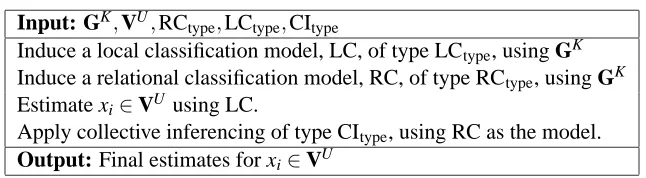
Input: GK,VU,RC
type,LCtype,CItype
Induce a local classification model, LC, of type LCtype, using GK
Induce a relational classification model, RC, of type RCtype, using GK
Estimate xi∈VU using LC.
Apply collective inferencing of type CItype, using RC as the model.
Output: Final estimates for xi∈VU
Table 2: High-level pseudo-code for the core routine of the Network Learning Toolkit.
pendencies such as homophily are modeled when the conditional modeling for a particular variable includes instantiations of the same variable from linked nodes. Relational extensions to Markov networks (Pearl, 1988) also can model arbitrary autocorrelation dependencies. In relational Markov networks (RMNs, Taskar et al., 2002) the clique potential functions are based on functional tem-plates, each of which is a (learned, class-conditional) probability function based on a user-specified set of relations. In associative Markov networks (AMNs, Taskar et al., 2004) autocorrelation of labels is explicitly modeled by extending the generalized Potts model (Potts, 1952) (specifically, to allow different labels to have different penalties). Of particular interest, exact inference can be per-formed in AMNs (formulated as a quadratic programming problem for binary classification, which can be relaxed for multi-class problems).
These methods for network classification use only a few of the many relational learning tech-niques. There are many more, for example from the rich literature of inductive logic programming (ILP, such as, De Raedt et al., 2001; Dzeroski and Lavrac, 2001; Kramer et al., 2001; Flach and Lachiche, 2004; Richardson and Domingos, 2006), or based on using relational database joins to generate relational features (e.g., Perlich and Provost, 2003; Popescul and Ungar, 2003; Perlich and Provost, 2006).
4. Network Learning Toolkit (NetKit-SRL)
NetKit is designed to accommodate the interchange of components and the introduction of new components. As outlined in Section 3.2, the node-centric learning framework comprises three main components: the relational classifier, the local classifier and collective inference. Any local clas-sifier can be paired with any relational clasclas-sifier, which can then be combined with any collective inference method. NetKit’s core routine is simple and is outlined in Table 2; it consists of these five general modules:
1. Input: This module reads data into a memory-resident graph G.
2. Local classifier inducer: Given as training data VK, this module returns a model
M
Lthat will estimate xi using only attributes of a node vi∈VU. Ideally,M
Lwill estimate a probability distribution over the possible values for xi.3. Relational classifier inducer: Given GK, this module returns a model
M
Rthat will estimate
4. Collective Inferencing: Given a graph G possibly with some xi known, a set of prior esti-mates for xU, and a relational model
M
R, this module applies collective inferencing to esti-mate xU.5. Weka Wrapper: This module is a wrapper for Weka5 (Witten and Frank, 2000) and can convert the graph representation of viinto an entity that can either be learned from or be used to estimate xi. NetKit can use a Weka classifier either as a local classifier or as a relational classifier (by using various aggregation methods to summarize the values of attributes in
N
i).The current version of NetKit-SRL, while able to read in heterogeneous graphs, only supports classification in graphs consisting of a single type of node. Algorithms based on expectation max-imization are possible to implement through the NetKit collective inference module, by having the collective inference module repeatedly apply a relational classifier to learn a new relational model and then apply the new relational model to G (rather than repeatedly apply the same learned model at every iteration).
The rest of this section describes the particular relational classifiers and collective inference methods implemented in NetKit for the case study. First, we describe the four (univariate6)
rela-tional classifiers. Then, we describe the three collective inference methods.
4.1 Relational Classifiers
All four relational classifiers take advantage of the first-order Markov assumption on the network: only a node’s local neighborhood is necessary for classification. The univariate case renders this assumption particularly restrictive: only the class labels of the local neighbors are necessary. The local network is defined by the user, analogous to the user’s definition of the feature set for proposi-tional learning. Entities whose class labels are not known are either ignored or are assigned a prior probability, depending upon the choice of local classifier.
4.1.1 WEIGHTED-VOTERELATIONALNEIGHBORCLASSIFIER(WVRN)
The case study’s simplest classifier (Macskassy and Provost, 2003)7 estimates class-membership probabilities by assuming the existence of homophily (see Section 3.4).
Definition. Given vi∈VU, the weighted-vote relational-neighbor classifier (wvRN) estimates
P(xi|
N
i)as the (weighted) mean of the class-membership probabilities of the entities inN
i:P(xi=c|
N
i) = 1Zv
∑
j∈Niwi,j·P(xj=c|
N
j),where Z is the usual normalizer. This can be viewed simply as an inference procedure, or as a probability model. In the latter case, it corresponds exactly to the Gaussian-field model discussed below in Section 3.5.2. How to conduct the inference/estimate the model falls on the collective inference procedure.
4.1.2 CLASS-DISTRIBUTIONRELATIONALNEIGHBORCLASSIFIER(CDRN)
The simple wvRN assumes that neighboring class labels were likely to be the same. Learning a model of the distribution of neighbor class labels is more flexible, and may lead to better discrimi-nation. Following Perlich and Provost (2003, 2006), and in the spirit of Rocchio’s method (Rocchio, 1971), we define node vi’s class vector CV(vi)to be the vector of summed linkage weights to the various (known) classes, and class c’s reference vector RV(c)to be the average of the class vectors for nodes known to be of class c. Specifically:
CV(vi)k=
∑
vj∈Ni,xj=ck
wi,j, (1)
where CV(vi)k represents the kth position in the class vector and ck ∈
X
is the kth class. Based on these class vectors, the reference vectors can then be defined as the normalized vector sum:RV(c) = 1
|VK
c|vi
∑
∈VKcCV(vi), (2)
where VKc ={vi|vi∈VK,xi=c}.
For the case study, during training, neighbors in VUare ignored. For prediction, estimated class membership probabilities are used for neighbors in VU, and Equation 1 becomes:
CV(vi)k=
∑
vj∈Ni
wi,j·P(xj=ck|
N
j). (3)Definition. Given vi ∈VU, the class-distribution relational-neighbor classifier (cdRN) esti-mates the probability of class membership, P(xi=c|
N
i), by the normalized vector similarity be-tween vi’s class vector and class c’s reference vector:P(xi=c|
N
i) =sim(CV(vi),RV(c)),where sim(a,b)is any vector similarity function (L1, L2, cosine, etc.), normalized to lie in the range [0,1]. For the results presented below, we use cosine similarity.
As with wvRN, Equation 3 is a recursive definition, and therefore the value of P(xj=c|
N
j)is approximated by the “current” estimate as defined by the selected collective inference technique.4.1.3 NETWORK-ONLY BAYESCLASSIFIER(NBC)
NetKit’s network-only Bayes classifier (nBC) is based on the algorithm described by Chakrabarti et al. (1998). To start, assume there is a single node vi in VU. The nBC uses multinomial naive Bayesian classification based on the classes of vi’s neighbors.
P(xi=c|
N
i) =P(
N
i|c)·P(c)P(
N
i) ,where
P(
N
i|c) = 1Zv
∏
j∈Niwhere Z is a normalizing constant and ˜xj is the class observed at node vj. As usual, because P(
N
i) is the same for all classes, normalization across the classes allows us to avoid explicitly computing it.We call nBC “network-only” to emphasize that in the application to the univariate case study below, we do not use local attributes of a node. As discussed above, Chakrabarti et al. initialize nodes’ priors based on a naive Bayes model over the local document text and add a text-based term to the node probability formula.8 In the univariate setting, local text is not available. We therefore use the same scheme as for the other relational classifiers: initialize unknown labels as decided by the local classifier being used (in our study: either the class prior or ’null’, depending on the collective inference component, as described below). If a neighbor’s label is ’null’, then it is ignored for classification. Also, Chakrabarti et al. differentiated between incoming and outgoing links, whereas we do not. Finally, Chakrabarti et al. do not mention how or whether they account for possible zeros in the estimations of the marginal conditional probabilities; we apply traditional Laplace smoothing where m=|
X
|, the number of classes.The foregoing assumes all neighbor labels are known. When the values of some neighbors are unknown, but estimations are available, we follow Chakrabarti et al. (1998) and perform a Bayesian combination based on (estimated) configuration priors and the entity’s known neighbors. Chakrabarti et al. (1998) describe this procedure in detail. For our case study, such an estimation is necessary only when using relaxation labeling (described below).
4.1.4 NETWORK-ONLY LINK-BASEDCLASSIFICATION(NLB)
The final relational classifier used in the case study is a network-only derivative of the link-based classifier (Lu and Getoor, 2003). The network-only Link-Based classifier (nLB) creates a feature vector for a node by aggregating the labels of neighboring nodes, and then uses logistic regression to build a discriminative model based on these feature vectors. This learned model is then applied to estimate P(xi=c|
N
i). As with the nBC, the difference between the “network-only” link-based classifier and Lu and Getoor’s version is that for the univariate case study we do not consider local attributes (e.g., text).As described above, Lu and Getoor (2003) considered various aggregation methods: existence (binary), the mode, and value counts. The last aggregation method, the count model, is equivalent to the class vector CV(vi)defined in Equation 3. This was the best performing method in the study by Lu and Getoor, and is the method on which we base nLB. The logistic regression classifier used by nLB is the multiclass implementation from Weka version 3.4.2.
We made one minor modification to the original link-based classifier. Perlich (2003) argues that in different situations it may be preferable to use either vectors based on raw counts (as given above) or vectors based on normalized counts. We did preliminary runs using both. The normalized vectors generally performed better, and so we use them for the case study.
4.2 Collective Inference Methods
This section describes three collective inferencing methods implemented in NetKit and used in the case study. As described above, given (i) a network initialized by the local model, and (ii) a relational model, a collective inference method infers a set of class labels for xU. Depending
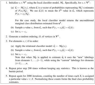
1. Initialize vi∈VUusing the local classifier model,ML. Specifically, for vi∈VU:
(a) cbi←ML(vi), wherecbiis a vector of probabilities representingML’s estimates
of P(xi|Ni). We use cbi(k) to mean the kth value in cbi, which represents P(xi=ck|Ni).
For the case study, the local classifier model returns the unconditional marginal class distribution estimated from xK.
(b) Sample a value csfromcbi, such that P(cs=ck|cbi) =cbi(k).
(c) Set xi←cs.
2. Generate a random ordering, O, of vertices in VU.
3. For elements vi∈O in order:
(a) Apply the relational classifier model:cbi←MR(vi).
(b) Sample a value csfromcbi, such that P(cs=ck|cbi) =cbi(k).
(c) Set xi←cs.
Note that when MR is applied to estimate cbi it uses the “new” labelings from elements 1, . . . ,(i−1), while using the “current” labelings for elements
(i+1), . . . ,n.
4. Repeat prior step 200 times without keeping any statistics. This is known as the burnin period.
5. Repeat again for 2000 iterations, counting the number of times each Xiis assigned
a particular value c∈X. Normalizing these counts forms the final class probability estimates.
Table 3: Pseudo-code for Gibbs sampling.
on the application, the goal ideally would be to infer the class labels with either the maximum joint probability or the maximum marginal probability for each node. Alternatively, if estimates of entities’ class-membership probabilities are needed, the collective inference method estimates the marginal probability distribution P(Xi=c|GK,Λ)for each Xi ∈xU and c∈
X
, whereΛstands for the priors returned by the local classifier.4.2.1 GIBBSSAMPLING (GS)
Gibbs sampling (Geman and Geman, 1984) is commonly used for collective inferencing with re-lational learning systems. The algorithm is straightforward and is shown in Table 3.9 The use of 200 and 2000 for the burnin period and number of iterations are commonly used values.10 Ideally, we would iterate until the estimations converge. Although there are convergence tests for the Gibbs sampler, they are neither robust nor well understood (cf., Gilks et al., 1995), so we simply use a fixed number of iterations.
9. This instance of Gibbs sampling uses a single random ordering (“chain”), as this is what we used in the case study. In the case study, averaging over 10 chains (the default in NetKit) had no effect on the final accuracies.
1. For vi∈VU, initialize the prior:cbi(0)←ML(vi), wherecbiis defined as in Table 3.
For the case study, the local classifier model returns the unconditional marginal class distribution estimated from xK.
2. For elements vi∈VU:
(a) Estimate xiby applying the relational model:
b
ci(t+1)←MR(v(it)), (4)
where MR(v(it)) denotes using the estimates cbj(t) for vj∈Ni, and t is the
iteration count. This has the effect that all predictions are done pseudo-simultaneously based on the state of the graph after iteration t.
3. Repeat for T iterations, where T =99 for the case study.bc(T)will comprise the final class probability estimations.
Table 4: Pseudo-code for relaxation labeling.
Notably, because all nodes are assigned a class at every iteration, when Gibbs sampling is used the relational models will always see a fully labeled/classified neighborhood, making prediction straightforward. For example, nBC does not need to compute its Bayesian combination (see Sec-tion 4.1.3).
4.2.2 RELAXATIONLABELING(RL)
The second collective inferencing method used in the study is relaxation labeling, based on the method of Chakrabarti et al. (1998). Rather than treat G as being in a specific labeling “state” at every point (as Gibbs sampling does), relaxation labeling retains the uncertainty, keeping track of the current probability estimations for xU. The relational model must be able to use these estimations. Further, rather than estimating one node at a time and updating the graph right away, relaxation labeling “freezes” the current estimations so that at step t+1 all vertices will be updated based on the estimations from step t. The algorithm is shown in Table 4.
Preliminary runs showed that relaxation labeling sometimes does not converge, but rather ends up oscillating between two or more graph states.11 NetKit performs simulated annealing—on each subsequent iteration giving more weight to a node’s own current estimate and less to the influence of its neighbors.
The new updating step, replacing Equation 4 is:
b
ci(t+1)=β(t+1)·
M
R(vi(t)) + (1−β(t+1))·cbi(t), whereβ0 = k,
β(t+1) = β(t)·α,
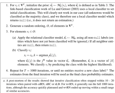
1. For vi∈VU, initialize the prior:cbi←ML(vi), wherecbiis defined as in Table 3. The
link-based classification work of Lu and Getoor (2003) uses a local classifier to set initial classifications. This will clearly not work in our case (all unknowns would be classified as the majority class), and we therefore use a local classifier model which returnsnull(i.e., it does not return an estimation.)
2. Generate a random ordering, O, of elements in VU.
3. For elements vi∈O:
(a) Apply the relational classifier model,cbi←MR, using all non-nulllabels
(en-tities which have not yet been classified will be ignored.) If all neighbor enti-ties arenull, then returnnull.
(b) Classify vi:
xi=ck,k=argmaxjcbi(j),
where cbi(j)is the jth value in vector cbi. (Remember, cbi is a vector of|X|
elements. We classify viby predicting the class with the highest likelihood).
4. Repeat for T=1000 iterations, or until no entities receive a new class label.a The estimates from the final iteration will be used as the final class probability estimates.
a. A post-mortem of the results showed that iterative classification often stopped within 10−20 iterations when paired with cdRN, nBC or nLB. For wvRN, it generally ran the full 1000 itera-tions, although the accuracy quickly plateaued and wvRN ended up moving within a small range of similar accuracies.
Table 5: Pseudo-code for Iterative classification.
where k is a constant between 0 and 1, which for the case study we set to 1.0, andα is a decay constant, which we set to 0.99. Preliminary testing showed that final performance is very robust as long as 0.9<α<1. Smaller values ofαcan lead to neighbors losing their influence too quickly, which can hurt performance when only very few labels are known. A post-mortem of the results showed that the accuracies often converged within the first 20 iterations.
4.2.3 ITERATIVECLASSIFICATION(IC)
The third and final collective inferencing method implemented in NetKit and used in the case study is the variant of iterative classification described in the work on link-based classification (Lu and Getoor, 2003) and shown in Table 5. As with Gibbs sampling, the relational model never sees uncertainty in the labels of (neighbor) entities. Either the label of a neighbor isnulland ignored (which only happens in the first iteration or if all its neighbors are also null), or it is assigned a definite label.
5. Case Study
and inference in homogeneous networks, comparing alternative techniques that have not before been compared systematically, if at all. The setting for the case study is simple: For some entities in the network, the value of xiis known; for others it must be estimated.
Univariate classification, albeit a simplification for many domains, is important for several rea-sons. First, it is a representation that is used in some applications. Above we mentioned fraud detec-tion; as a specific example, a telephone account that calls the same numbers as a known fraudulent account (and hence the accounts are connected through these intermediary numbers) is suspicious (Fawcett and Provost, 1997; Cortes et al., 2001). For phone fraud, univariate network classification often provides alarms with reasonable coverage and remarkably low false-positive rates. Gener-ally speaking, a homogeneous, univariate network is an inexpensive (in terms of data gathering, processing, storage) approximation of many complex networked data problems. Fraud detection applications certainly do have a variety of additional attributes of importance; nevertheless, univari-ate simplifications are very useful and are used in practice.
The univariate case also is important scientifically. It isolates a primary difference between networked data and non-networked data, facilitating the analysis and comparison of relevant clas-sification and learning methods. One thesis of this study is that there is considerable information inherent in the structure of the networked data and that this information can be readily taken advan-tage of, using simple models, to estimate the labels of unknown entities. This thesis is tested by isolating this characteristic—namely ignoring any auxiliary attributes and only allowing the use of known class labels—and empirically evaluating how well univariate models perform in this setting on benchmark data sets.
Considering homogeneous networks plays a similar role. Although the domains we consider have obvious representations consisting of multiple entity types and edges (e.g., people and papers for node types and same-author-as and cited-by as edge types in a citation-graph domain), a homo-geneous representation is much simpler. In order to assess whether a more complex representation is worthwhile, it is necessary to assess standard techniques on the simpler representation (as we do in this case study). Of course, the way a network is “homogenized” may have a considerable effect on classification performance. We will revisit this below in Section 5.3.6.
5.1 Data
The case study reported in this paper makes use of 12 benchmark data sets from four domains that have been the subject of prior study in machine learning. As this study focuses on networked data, any singleton (disconnected) entities in the data were removed. Therefore, the statistics we present may differ from those reported previously.
5.1.1 IMDB
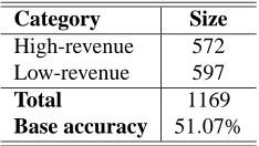
Networked data from the Internet Movie Database (IMDb)12 have been used to build models pre-dicting movie success as determined by box-office receipts (Jensen and Neville, 2002a). Following the work of Neville et al. (2003), we focus on movies released in the United States between 1996 and 2001 with the goal of estimating whether the opening weekend box-office receipts “will” ex-ceed $2 million (Neville et al., 2003). Obtaining data from the IMDb web-site, we identified 1169 movies released between 1996 and 2001 that we were able to link up with a revenue classification
Category Size High-revenue 572 Low-revenue 597
Total 1169
Base accuracy 51.07%
Table 6: Class distribution for the IMDb data set.
Category Size
Case-based 402
Genetic Algorithms 551 Neural Networks 1064 Probabilistic Methods 529 Reinforcement Learning 335
Rule Learning 230
Theory 472
Total 3583
Base accuracy 29.70%
Table 7: Class distribution for the cora data set.
in the database given to us by the authors of the original study. The class distribution of the data set is shown in Table 6.
We link movies if they share a production company, based on observations from previous work (Macskassy and Provost, 2003).13 The weight of an edge in the resulting graph is the number of production companies two movies have in common. Notably, we ignore the temporal aspect of the movies in this study, simply labeling movies at random for the training set. This can result in a movie in the test set being released earlier than a movie in the training set.
5.1.2 CORA
The cora data set (McCallum et al., 2000) comprises computer science research papers. It includes the full citation graph as well as labels for the topic of each paper (and potentially sub- and sub-sub-topics).14 Following a prior study (Taskar et al., 2001), we focused on papers within the machine learning topic with the classification task of predicting a paper’s sub-topic (of which there are seven). The class distribution of the data set is shown in Table 7.
Papers can be linked if they share a common author, or if one cites the other. Following prior work (Lu and Getoor, 2003), we link two papers if one cites the other. The weight of an edge would normally be one unless the two papers cite each other (in which case it is two—there can be no other weight for existing edges).
13. And on a suggestion from David Jensen.
Number of web-pages
Class Cornell Texas Washington Wisconsin
student 145 163 151 155
not-student 201 171 283 193
Total 346 334 434 348
Base accuracy 58.1% 51.2% 60.8% 55.5%
Table 8: Class distribution for the WebKB data set using binary class labels.
5.1.3 WEBKB
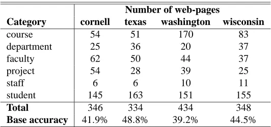
The third domain we draw from is based on the WebKB Project (Craven et al., 1998).15 It consists of sets of web pages from four computer science departments, with each page manually labeled into 7 categories: course, department, faculty, project, staff, student, or other. As with other work (Neville et al., 2003; Lu and Getoor, 2003), we ignore pages in the “other” category except as described below.
From the WebKB data we produce eight networked data sets for within-network classification. For each of the four universities, we consider two different classification problems: the six-class problem, and following a prior study, the binary classification task of predicting whether a page belongs to a student (Neville et al., 2003).16 The binary task results in an approximately balanced
class distribution.
Following prior work on web-page classification, we link two pages by co-citations (if x links to z and y links to z, then x and y are co-citing z) (Chakrabarti et al., 1998; Lu and Getoor, 2003). To weight the link between x and y, we sum the number of hyperlinks from x to z and separately the number from y to z, and multiply these two quantities. For example, if student x has 2 edges to a group page, and a fellow student y has 3 edges to the same group page, then the weight along that path between those 2 students would be 6. This weight represents the number of possible co-citation paths between the pages. Co-co-citation relations are not uniquely useful to domains involving documents; for example, as mentioned above, for phone-fraud detection bandits often call the same numbers as previously identified bandits. We chose co-citations for this case study based on the prior observation that a student is more likely to have a hyperlink to her advisor or a group/project page rather than to one of her peers (Craven et al., 1998).17
To produce the final data sets, we extracted the pages that have at least one incoming and one outgoing link. We removed pages in the “other” category from the classification task, although they were used as “background” knowledge—allowing 2 pages to be linked by a path through an “other” page. For the binary tasks, the remaining pages were categorized into either student or not-student. The composition of the data sets is shown in Tables 8 and 9.
5.1.4 INDUSTRYCLASSIFICATION
The final domain we draw from involves classifying companies by industry sector. Companies are linked via cooccurrence in text documents. We use two different data sets, representing different
15. We use the WebKB-ILP-98 data.
16. It turns out that the relative performance of the methods is quite different on these two variants.
Number of web-pages
Category cornell texas washington wisconsin
course 54 51 170 83
department 25 36 20 37
faculty 62 50 44 37
project 54 28 39 25
staff 6 6 10 11
student 145 163 151 155
Total 346 334 434 348
Base accuracy 41.9% 48.8% 39.2% 44.5%
Table 9: Class distribution for the WebKB data set using six-class labels.
Number of companies Sector industry-yh industry-pr
Basic Materials 104 83
Capital Goods 83 78
Conglomerates 14 13
Consumer Cyclical 99 94
Consumer NonCyclical 60 59
Energy 71 112
Financial 170 268
Healthcare 180 279
Services 444 478
Technology 505 609
Transportation 38 47
Utilities 30 69
Total 1798 2189
Base accuracy 28.1% 27.8%
Table 10: Class distribution for the industry-yh and industry-pr data sets.
sources and distributions of documents and different time periods (which correspond to different topic distributions).
INDUSTRYCLASSIFICATION(YH)
As part of a study of activity monitoring, Fawcett and Provost (1999) collected 22,170 business news stories from the web between 4/1/1999 and 8/4/1999. Following the study by Bernstein et al. (2003), we placed an edge between two companies if they appeared together in a story. The weight of an edge is the number of such cooccurrences found in the complete corpus. The resulting network comprises 1798 companies that cooccurred with at least one other company. To classify a company, we used Yahoo!’s 12 industry sectors. Table 10 shows the details of the class memberships.
INDUSTRYCLASSIFICATION(PR)
together in a press release. The weight of an edge is the number of such cooccurrences found in the complete corpus. The resulting network comprises 2189 companies that cooccurred with at least one other company. To classify a company, we use the same classification scheme from Yahoo! as before. Table 10 shows the details of the class memberships.
5.2 Experimental Methodology
NetKit allows for any combination of a local classifier (LC), a relational classifier (RC) and a collective inferencing method (CI). If we consider an LC-RC-CI configuration to be a complete
network-classification method, we have 12 to compare on each data set. Since, for this paper, the
local classifier component is directly tied to the collective inference component (our local classifier components determine priors based on which collective inference component is being used), we henceforth consider a network-classification method to be an RC-CI configuration.
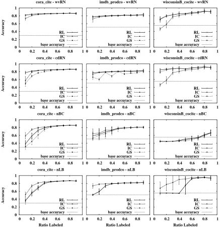
We first verify that the network structure alone (linkages plus known class labels) often con-tains a considerable amount of useful information for entity classification. We vary from 10% to 90% the percentage of nodes in the network for which class membership is known initially.18 The study assesses: (1) whether the network structure enables accurate classification; (2) how much prior information is needed in order to perform well, and (3) whether there are regular patterns of improvement across methods as the percentage of initially known labels increases.
Accuracy is averaged over 10 runs. Specifically, given a data set, G= (V,E), the subset of entities with known labels VK (the “training” data set19) is created by selecting a class-stratified random sample of(100×r)% of the entities in V. The test set, VU, is then defined as V−VK. We prune VU by removing all nodes in zero-knowledge components—nodes for which there is no path to any node in VK. We use the same 10 training/test partitions for each network-classification method. Although it would be desirable to keep the test data disjoint (and therefore independent) as done in traditional machine learning via methods such as cross-validation, this is not applicable for within-network learning. We keep the test node sets disjoint as much as possible between the different runs. For example, at r=0.90 (90% labeled data), our sets of training and testing nodes follow standard class-stratified 10-fold cross-validation.
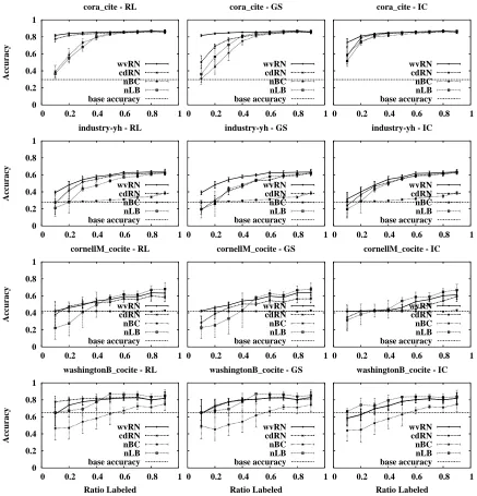
5.3 Results
0 0.2 0.4 0.6 0.8 1
0 0.2 0.4 0.6 0.8 1
Accuracy Ratio Labeled cora_cite 0 0.2 0.4 0.6 0.8 1
0 0.2 0.4 0.6 0.8 1
Accuracy Ratio Labeled cornellB_cocite 0 0.2 0.4 0.6 0.8 1
0 0.2 0.4 0.6 0.8 1
Accuracy Ratio Labeled cornellM_cocite 0 0.2 0.4 0.6 0.8 1
0 0.2 0.4 0.6 0.8 1
Accuracy Ratio Labeled imdb_prodco 0 0.2 0.4 0.6 0.8 1
0 0.2 0.4 0.6 0.8 1
Accuracy Ratio Labeled texasB_cocite 0 0.2 0.4 0.6 0.8 1
0 0.2 0.4 0.6 0.8 1
Accuracy Ratio Labeled texasM_cocite 0 0.2 0.4 0.6 0.8 1
0 0.2 0.4 0.6 0.8 1
Accuracy Ratio Labeled industry-pr 0 0.2 0.4 0.6 0.8 1
0 0.2 0.4 0.6 0.8 1
Accuracy Ratio Labeled washingtonB_cocite 0 0.2 0.4 0.6 0.8 1
0 0.2 0.4 0.6 0.8 1
Accuracy Ratio Labeled washingtonM_cocite 0 0.2 0.4 0.6 0.8 1
0 0.2 0.4 0.6 0.8 1
Accuracy Ratio Labeled industry-yh 0 0.2 0.4 0.6 0.8 1
0 0.2 0.4 0.6 0.8 1
Accuracy Ratio Labeled wisconsinB_cocite 0 0.2 0.4 0.6 0.8 1
0 0.2 0.4 0.6 0.8 1
Accuracy
Ratio Labeled wisconsinM_cocite