Evolving GPU Machine Code

(1)

Evolving GPU Machine Code

Cleomar Pereira da Silva cleomar.silva@ifc-videira.edu.br Department of Electrical Engineering

Pontifical Catholic University of Rio de Janeiro (PUC-Rio) Rio de Janeiro, RJ 22451-900, Brazil

Department of Education Development

Federal Institute of Education, Science and Technology - Catarinense (IFC) Videira, SC 89560-000, Brazil

Douglas Mota Dias douglasm@ele.puc-rio.br

Department of Electrical Engineering

Cristiana Bentes cris@eng.uerj.br

Department of Systems Engineering State University of Rio de Janeiro (UERJ) Rio de Janeiro, RJ 20550-013, Brazil

Marco Aur´elio Cavalcanti Pacheco marco@ele.puc-rio.br Department of Electrical Engineering

Leandro Fontoura Cupertino fontoura@irit.fr

Toulouse Institute of Computer Science Research (IRIT) University of Toulouse

118 Route de Narbonne

F-31062 Toulouse Cedex 9, France

Editor:Una-May O’Reilly

Abstract

Parallel Graphics Processing Unit (GPU) implementations of GP have appeared in the lit-erature using three main methodologies: (i)compilation, which generates the individuals in GPU code and requires compilation; (ii)pseudo-assembly, which generates the individuals in an intermediary assembly code and also requires compilation; and (iii) interpretation, which interprets the codes. This paper proposes a new methodology that uses the concepts of quantum computing and directly handles the GPU machine code instructions. Our methodology utilizes a probabilistic representation of an individual to improve the global search capability. In addition, the evolution in machine code eliminates both the overhead of compiling the code and the cost of parsing the program during evaluation. We obtained up to 2.74 trillion GP operations per second for the 20-bit Boolean Multiplexer benchmark. We also compared our approach with the other three GPU-based acceleration methodolo-gies implemented for quantum-inspired linear GP. Significant gains in performance were obtained.

(2)

1. Introduction

Genetic programming (GP) is a metaheuristic method to automatically generate computer programs or key subcomponents (Banzhaf et al., 1997; Koza, 1992; Poli et al., 2008). Its functionality is based on the Darwinian principle of natural selection, in which a popula-tion of computer programs, or individuals, is maintained and modified based on genetic variation. The individuals are then evaluated according to a fitness function to reach a better solution. GP has been successfully applied to a variety of problems, such as auto-matic design, pattern recognition, robotic control, data mining, and image analysis (Koza, 1992, 1994; Tackett, 1993; Busch et al., 2002; Harding and Banzhaf, 2008; Langdon, 2010a). However, the evaluation process is time consuming. The computational power required by GP is enormous, and high-performance techniques have been used to reduce the computa-tion time (Andre and Koza, 1996; Salhi et al., 1998). GP parallelism can be exploited on two levels: multiple individuals can be evaluated simultaneously, or multiple fitness cases for one individual can be evaluated in parallel. These approaches have been implemented in multiprocessor machines and computer clusters (Page et al., 1999; Turton et al., 1996; Bennett III et al., 1999).

The recent emergence of general-purpose computing on Graphics Processing Units (GPUs) has provided the opportunity to significantly accelerate the execution of many costly algo-rithms, such as GP algorithms. GPUs have become popular as accelerators due to their high computational power, low cost, impressive floating-point capabilities, and high mem-ory bandwidth. These characteristics make them attractive platforms to accelerate GP computations, as GP has a fine-grained parallelism that is suitable for GPU computation.

The power of the GPU to accelerate GP has been exploited in previous studies. We di-vide these efforts into three main methodologies: (i)compilation(Chitty, 2007; Harding and Banzhaf, 2007, 2009; Langdon and Harman, 2010); (ii) pseudo-assembly (Cupertino et al., 2011; Pospichal et al., 2011; Lewis and Magoulas, 2011); and (iii) interpretation (Lang-don and Banzhaf, 2008a; Lang(Lang-don and Harrison, 2008; Robilliard et al., 2009; Wilson and Banzhaf, 2008). In the compilationmethodology, each evolved program, or GP individual, is compiled for the GPU machine code and then evaluated in parallel on the GPU. In the pseudo-assembly methodology, the individuals are generated in the pseudo-assembly code of the GPU, and a just-in-time (JIT) compilation is performed for each individual to gen-erate the GPU machine code, which is evaluated in parallel on the GPU. In theinterpreter methodology, an interpreter that can run programs immediately is used. The individuals are evaluated in parallel on the GPU.

(3)

code, allowing large data sets to be considered. Nevertheless, the programs still need to be compiled, and the compilation time must be considered as part of the overall GP pro-cess. The interpreter methodology differs from the compilation methodology in that the interpreter is compiled once and reused millions of times. This approach eliminates the compilation overhead but includes the cost of parsing the evolved program. Theinterpreter methodology typically works well for shorter programs and smaller training cases.

In this work, we propose a new methodology for using GPUs in the GP evolution process. We used a quantum-inspired evolutionary algorithm (QEA) that handles the instructions of the GPU machine code directly. QEAs represent one of the most recent advances in evolutionary computation (Zhang, 2011). QEAs are based on quantum mechanics, particu-larly the concepts of the quantum bit and the superposition of states. QEAs can represent diverse individuals in a probabilistic manner. By this mechanism, QEAs offer an evolu-tionary mechanism that is different and, in some situations, more effective than traditional evolutionary algorithms. The quantum probabilistic representation reduces the number of chromosomes required to guarantee adequate search diversity. In addition, the use of quantum interference provides an effective approach to achieve fast convergence to the best solution due to the inclusion of an individual’s past history. It offers a guide for the popu-lation of individuals that helps to exploit the current solution’s neighborhood.

Our methodology is called GPU machine code genetic programming, GMGP, and is based on linear genetic programming (LGP) (Nordin, 1998; Brameier and Banzhaf, 2007; Oltean et al., 2009). In LGP, each program is a linear sequence of instructions. LGP is the most appropriate for machine code programs, as computer architectures require programs to be provided as linear sequences. Computers do not naturally run tree-shaped programs. Tree-based GP must employ compilers or interpreters (Poli et al., 2008).

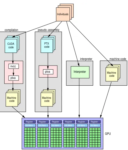
GMGP performs the evolution by modifying the GPU machine code, thus eliminating the time spent compiling the individuals while also avoiding the interpretation overhead. The individuals are generated on the CPU, and the individuals are evaluated in parallel on the GPU. The evaluation process is performed with a high level of parallelism: individuals are processed in parallel, and the fitness cases are simultaneously evaluated in parallel. Figure 1 illustrates the GPU-accelerated GP methodologies.

(4)

ptxa nvcc

ptxa Interpreter

Sh Mem Register

Sh Mem Register Sh Mem

Register Sh Mem Register

Sh Mem Register

pseudo−assembly compilation

interpreter machine code

GPU CUDA

code

PTX code

Machine code

Machine code Individuals

Figure 1: The different GP methodologies for GPU, considering the Nvidia technology. In the compilation methodology, a CUDA kernel is generated from each individual. The kernels are compiled in two main steps using thenvccandptxascompilers. In the pseudo-assembly methodology, pseudo-assembly codes (PTX) are generated from each individual and compiled using the ptxas compiler. In the interpreter methodology, each individual’s information is used by the interpreter to execute the program. The proposed machine code methodology generates a machine code program directly from each individual.

2. Related Work

Several approaches to accelerate GP on GPUs have been proposed in the literature. Harding and Banzhaf (2007) and Chitty (2007) were the first to present GP implementations on a GPU. Both works proposed compiler methodologies using tree-based GP. They obtained modest performance gains when small fitness cases were tested due to the overhead of transferring data to the GPU. Considerable performance gains were obtained for larger problems and when the compiled GP program was run many times.

(5)

the function set. The experimental results indicated moderate speedups but demonstrated performance gains even for very small programs. The same GPU SIMD interpreter was used by Langdon and Harrison (2008), who successfully applied GP to predict the breast cancer survival rate beyond ten years.

Robilliard et al. (2009) also studied the interpreter methodology, with a focus on avoiding the overhead of conditional instructions when interpreting the entire population at once. They proposed an interpreter that evaluates each GP individual on a different thread block. Each thread block was mapped to a different GPU multiprocessor during execution, avoiding branches. Inside the thread block, all threads executed the same instruction over different data subsets. Their results indicated performance gains compared to the methodology proposed by Langdon and Banzhaf (2008a).

Harding and Banzhaf (2009) studied the compilation methodology. A cluster of GPUs was used to alleviate the program compilation overhead. The focus was on processing very large data sets by using the cluster nodes to compile the GPU code and execute the programs. Different combinations of compilation and execution nodes could be used. The project was developed to run on a multi-platform Windows/Linux cluster and used low-end GPUs. Speedups were obtained for very large data sets. However, the use of high-end GPUs did not necessarily lead to better results, as the primary bottleneck remained in the compilation phase.

Langdon and Harman (2010) used the compilation methodology to automatically create an Nvidia CUDA kernel. Numerous simplifications were employed, such as not evolving the shared memory and threading information. The best evolved parallel individual was capable of correct calculations, proving that it was possible to elaborate a methodology to evolve parallel code. However, it was not possible to automatically verify the speedup obtained compared to the sequential CPU version, and the compilation still remained the bottleneck.

Wilson and Banzhaf (2008) implemented an LGP for GPU using the interpreter method-ology on a video game console. In a previous work (Cupertino et al., 2011), we proposed a pseudo-assembly methodology, a modified LGP for GPU, called quantum-inspired lin-ear genetic programming on a general-purpose graphics processing unit (QILGP3U). The individual was created in the Nvidia pseudo-assembly code, PTX, and compiled for evalu-ation through JIT. Dynamic or JIT compilevalu-ation is performed in runtime and transformed the assembly code to machine code during the execution of the program. Several compi-lation phases were eliminated, and significant speedups were achieved for large data sets. Pospichal et al. (2011) also proposed a pseudo-assembly methodology with the evolution of PTX code using a grammar-based GP that ran entirely on the GPU.

The compilation time issue was addressed in a different manner by Lewis and Magoulas (2011). All population individuals were pre-processed to identify their similarities, and all of these similarities were grouped together. In this manner, repetitive compilation was eliminated, thus reducing the compilation time by a factor of up to 4.8.

(6)

3. Quantum Computing and Quantum-Inspired Algorithms

In a classical computer, a bit is the smallest information unit and can take a value of 0 or 1. In a quantum computer, the basic information unit is the quantum bit, called the qubit. A qubit can take the states|0i or |1i or a superposition of the two. This superposition of the two states is a linear combination of the states |0i and |1i and can be represented as follows:

|ψi=α|0i+β|1i, (1)

where |ψi is the qubit state , α and β are complex numbers, and |α|2 _and _|β|2 _{are the} probabilities that the qubit collapses to state 0 or 1, respectively, based on its observation (i.e., measurement). The unitary normalization guarantees the following:

|α|2+|β|2= 1| {α,β} ∈C. (2)

The superposition of states provides quantum computers with an incomparable degree of parallelism. This parallelism, when properly exploited, allows computers to perform tasks that are unfeasible in classical computers due to the prohibitive computational time.

Although quantum computing is promising in terms of processing capacity, there is still no technology for the actual implementation of a quantum computer, and there are only a few complex quantum algorithms.

Moore and Narayanan (1995) proposed a new approach to exploit the quantum comput-ing concepts. Instead of developcomput-ing new algorithms for quantum computers or attemptcomput-ing to make their use feasible, they proposed the idea of quantum-inspired computing. This new approach aims to create classical algorithms (i.e., running on classical computers) that utilize quantum mechanics paradigms to improve their problem-solving performance. In particular, quantum-inspired evolutionary algorithms (QEAs) have recently become a sub-ject of special interest in evolutionary computation. The linear superposition of states represented in a qubit allows QEA to represent diverse individuals probabilistically. QEAs belong to the class of estimation of distribution algorithms (EDAs) (Platel et al., 2009). The probabilistic mechanism provides QEAs with an evolutionary mechanism that has several advantages, such as global search capability and faster convergence and smaller population size than those of traditional evolutionary algorithms. These algorithms have already been successfully used to solve various problems, such as the knapsack problem (Han and Kim, 2002), ordering combinatorial optimization problems (Silveira et al., 2012), engineering op-timization problems (Alfares and Esat, 2006), image segmentation (Talbi et al., 2007), and image registration (Draa et al., 2004). See Zhang (2011) for more examples of QEAs and their applications.

3.1 Multilevel Quantum Systems

(7)

4. Quantum-Inspired Linear Genetic Programming

The proposed inspired GP methodology for GPUs is based on the quantum-inspired linear genetic programming (QILGP) algorithm proposed by Dias and Pacheco (2013). QILGP evolves machine code programs for the Intel x86 platform. It uses floating point instructions and works with data from the main memory (m) and/or eight FPU regis-ters (ST(i) | i∈[0..7]). The function set consists of addition, subtraction, multiplication, division, data transfer, trigonometric, and other arithmetic instructions. QILGP generates variable-sized programs by adding the NOP instruction to the instruction set. The code generation ignores any gene in which a NOP is present. Table 1 provides an example of a function set.

Each individual is represented by a linear sequence of machine code instructions. Each instruction can use one or zero arguments. The evaluation of a program requires the input data to be read from the main memory, which consists of the input variables of the problem and some optional constants supplied by the user. The input data are represented by a vector, such as

I = (V[0], V[1],1,2,3), (3)

whereV[0] andV[1] have the two input values of the problem (i.e., a fitness case) and 1, 2, and 3 are the three constant values.

The instructions are represented in QILGP by two tokens: the function token (FT), which represents the function, and theterminal token(TT), which represents the argument of the function. Each function has a single terminal. When a function has no terminal, its corresponding token value is ignored. Each token is an integer value that represents an index to the function set or terminal set.

4.1 Representation

QILGP is based on the following entities: thequantum individual, which represents the su-perposition of all possible programs for the defined search space, and theclassical individual (or individual), which represents the machine code program coded in the token values. A classical individual represents an individual of a traditional linear GP. In the observation phase of QILGP, each quantum individual is observed to generate one classical individual.

4.2 Observation

The chromosome of a quantum individual is represented by a list of structures called quan-tum genes. The observation of a quantum individual comprises the observations of all of its chromosome genes. The observation process consists of randomly generating a value r {r ∈R|0 ≤r ≤1} and searching for the interval in which r belongs in all possible states

(8)

Instruction Operation Arg.

NOP No operation

-FADD m ST(0)←ST(0) +m m

FADD ST(0), ST(i) ST(0)←ST(0) +ST(i) i

FADD ST(i), ST(0) ST(i)←ST(i) +ST(0) i

FSUBm ST(0)←ST(0)−m m

FSUB ST(0), ST(i) ST(0)←ST(0)−ST(i) i

FSUB ST(i), ST(0) ST(i)←ST(i)−ST(0) i

FMUL m ST(0)←ST(0)×m m

FMUL ST(0), ST(i) ST(0)←ST(0)×ST(i) i

FMUL ST(i), ST(0) ST(i)←ST(i)×ST(0) i

FXCH ST(i) ST(0)ST(i) (swap) i

FDIV m ST(0)←ST(0)÷m m

FDIV ST(0), ST(i) ST(0)←ST(0)÷ST(i) i

FDIV ST(i), ST(0) ST(i)←ST(i)÷ST(0) i

FABS ST(0)← |ST(0)| -FSQRT ST(0)←pST(0) -FSIN ST(0)←sinST(0) -FCOS ST(0)←cosST(0)

-Table 1: Functional description of the instructions. The first column presents the Intel x86 instructions. The second column presents the operations performed. The third column presents the argument of the instructions (m indexes memory positions, and iselects a register).

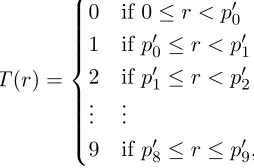
represented by 10 different states follows the function

T(r) =

        

       

0 if 0≤r < p0₀

1 ifp0₀ ≤r < p0₁

2 ifp0₁ ≤r < p0₂

.. . ...

9 ifp0₈ ≤r≤p0₉,

(4)

where{r ∈_R|0≤r≤1}is the randomly generated value with a uniform distribution and

T(r) returns the observed value for the token.

(9)

0 1 2

0.100 0.250 0.200

p0 p1 p2 3

0.125

p3

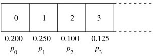
Figure 2: Illustration of a qudit implementation that represents Equation (6). Each state has an associated probability value and a token value. The observation process generates a random number r and selects one token based on the probability interval in whichr fits.

QILGP is inspired by multilevel quantum systems (Lanyon et al., 2008), and uses the qudit as the basic information unit. This information can be described by a state vector of

dlevels, wheredis the number of states in which the qudit can be measured. Accordingly,

drepresents the cardinality of the token. The state of a qudit is a linear superposition ofd

states and may be represented as follows:

|ψi=

d−1

X

i=0

αi|ii, (5)

where|αi|2 is the probability that the qudit collapses to stateiwhen observed.

For example, suppose that each instruction in Table 1 has a unique token value in

T = {0,1,2,3,...}. Equation (6) provides the state of a function qudit (FQ) whose state is given as follows:

|ψi= √1

5|0i+ 1

√

4|1i+ 1

√

10|2i+ 1

√

8|3i+. . . (6)

The probability of measuring the NOPinstruction (state |0i) is (1_/√₅₎2 _{= 0}_._{200, for} _FADD _m (state |1i) is (1_/√₄₎2 _{= 0}_._{250, for} _{FADD ST(0),ST(i)} _(state_|₂_i_{) is (}1_/√₁₀₎2 _{= 0}_._{100, and so} on. The qudit state of this example is implemented in a data structure as shown in Figure 2.

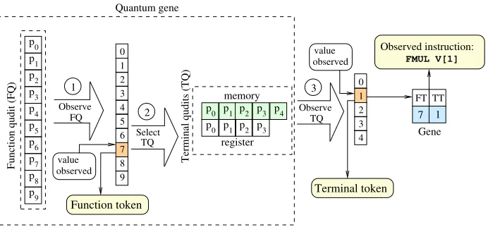
Figure 3 illustrates the creation of a classical gene by the observation of a quantum gene from an example based on Table 1 and the input vector I = (V[0], V[1],1,2,3) (Equation 3). This process can be explained by three basic steps, indicated by the numbered circles in Figure 3:

1. The FQ is observed, and the resulting value (e.g., 7) is assigned to the FT of this gene.

2. The FT value determines the terminal qudit (TQ) to be observed, as each instruction requires a different type of terminal: register or memory.

(10)

value observed Terminal token value observed FT TT 7 1 Gene Observed instruction: FMUL V[1] 1 p 0 p 1 p 2 p 3 4 p 5 6 p 7 p 8 p 9 p p 0 1 2 3 4

Function qudit (FQ)

2 Function token Select TQ TQ 3 Observe Observe FQ Quantum gene

Terminal qudits (TQ)

register memory p 4 p p

0 1 p2 p3

p p

0 1 p2 p3

5 7 8 9 6 0 1 2 3 4

Figure 3: The creation of a classical gene from the observation of a quantum gene. The FQ is observed, and the token value selected is 7. The memory qudit is selected in the TQ. The TQ is observed, and the TT value selected is 1. The observed instruction in this example is FMUL V[1], as ‘7’ is the FT value for this instruction (Table 1), and ‘1’ is the TT value that represents V[1] in the input vector I defined by Equation (3).

4.3 Evaluation of a Classical Individual

This process begins with the generation of a machine code program from the classical individual under evaluation, where its chromosome is sequentially traversed, gene by gene and token by token (both FTs and TTs), to serially generate the program body machine code related to the classical individual. Then, the program is executed for all fitness cases of the problem (i.e., samples of the training data set).

For each fitness case, the value assigned as the result of the fitness case is zero (V[0]←0) when the instructions FDIV require division by zero or the instructions FSQRT require the calculation of the square root of a negative number.

4.4 Quantum Operator

The quantum operator of QILGP manipulates the probability pi of a qudit, satisfying the

normalization condition Pd−1

i=0 |αi|2 = 1, where d is the qudit cardinality and |αi|2 = pi.

Operator P works in two main steps. First, it increases the given probability of a qudit as follows:

pi ←pi+s×(1−pi), (7)

where s is a parameter called step size, which can assume any real value between 0 and 1. The second step is to adjust the values of all of the probabilities of that qudit to satisfy the normalization condition. Thus, the operator modifies the state of a qudit by increasingpi of a value that is directly proportional tos. The asymptotic behavior of pi in

(11)

C_B

C₀ C₁ C₂ C₃

C₀ C₁ C₂ C₃ 3. Application of operator P

Classical population

Quantum population Population

1. Observation

Observed individuals

2. Sorting 4. Conditional

copy

Q₀ Q₁ Q₂ Q₃

obs obs obs obs

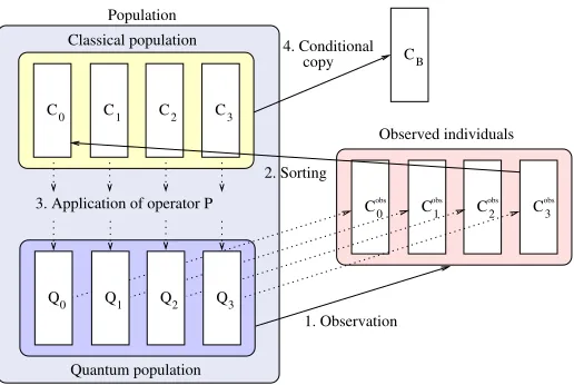
Figure 4: The four basic steps that characterize a generation of QILGP. With a population size of 4, the quantum individuals are observed and generate classical individuals. The classical individuals are sorted by their evaluations. The operatorP is applied to each quantum individual, using the classical individual as the reference. The best classical individual evaluated thus far is kept inCB.

cause the qudit to collapse, which could cause a premature convergence of the evolutionary search process.

QILGP has a hybrid population composed of a quantum population and classical pop-ulation, both of which comprise M individuals. QILGP also has M auxiliary classical individuals C_iobs, which result from observations of the quantum individuals Qi, where

1≤i≤M.

4.5 Evolutionary Algorithm

Figure 4 illustrates the four basic steps that characterize a generation of QILGP, with a population sizeM = 4. The algorithm works as follows:

1. Each of M quantum individuals is observed once, resulting in M classical individuals

C_iobs.

2. The individuals of the classical population and the observed individuals (auxiliary) are jointly sorted by their evaluations, ordered from best to worst, from C0 toCM−1. 3. The operatorP is applied to each quantum individualQi, taking their corresponding

individualCiin the classical population as a reference. Thus, at every new generation,

the application of this operator increases the probability that the observations of the quantum individuals generate classical individuals more similar to the best individuals found thus far.

4. If any classical individual evaluated in the current generation is better than the best classical individual evaluated previously, a copy is stored inCB, which keeps the best

(12)

5. GPU Architecture

GPUs are highly parallel, many-core processors typically used as accelerators for a host system. They provide tremendous computational power and have proven to be successful for general-purpose parallel computing in a variety of application areas. Although different manufacturers have developed GPUs in recent years, we have opted for GPUs from Nvidia due to their flexibility and availability.

An Nvidia GPU consists of a set of streaming multiprocessors (SMs), each consisting of a set of GPU cores. The memory in the GPU is organized as follows: a large global memory with high latency; a very fast, low-latency on-chip shared memory for each SM; and a private local memory for each thread. Data communication between the GPU and CPU is conducted via the PCIe bus. The CPU and GPU have separate memory spaces, referred to as the host memory and device memory, and the GPU-CPU transfer time is limited by the speed of the PCIe bus.

5.1 Programming Model

The Nvidia programming model is CUDA (Computer Unified Device Architecture) (Nvidia, 2013). CUDA is a C-based development environment that allows the programmer to de-fine special C functions, called kernels, which execute in parallel on the GPU by different threads. The GPU supports a large number of fine-grain threads. The threads are orga-nized into a hierarchy of thread grouping. The threads are divided into a two- or three-dimensionalgridof thread blocks. Each thread block is a two- or three-dimensional thread array. Thread blocks are executed on the GPU by assigning a number of blocks to be exe-cuted on a SM. Each thread in a thread block has a unique identifier, given by the built-in variables threadIdx.x, threadIdx.y, and threadIdx.z. Each thread block has an iden-tifier that distinguishes its position in the grid, given by the built-in variablesblockIdx.x, blockIdx.y, andblockIdx.z. The dimensions of the thread and thread block are specified at the time when the kernel is launched through the identifiers blockDim and gridDim, respectively.

(13)

5.2 Compilation

The compilation of a CUDA program is performed through the following stages. First, the CUDA front end,cudafe, divides the program into the C/C++ host code and GPU device code. The host code is compiled with a regular C compiler, such asgcc. The device code is compiled using the CUDA compiler,nvcc, generating an intermediate code in an assembly language called PTX (Parallel Thread Execution). PTX is a human-readable, assembly-like low-level programming language for Nvidia GPUs that is compiled and hides many of the machine details. PTX has been fully documented by Nvidia. The PTX code is then translated to the GPU binary code, CUBIN, using the ptxas compiler.

Unlike the PTX language, whose documentation has been made public, the CUBIN format is proprietary, and no information has been made available by Nvidia. All of the work performed with CUBIN requires reverse engineering. In addition, the manufacturer provides only the most basic elements of the underlying hardware architecture, and there are apparently no plans to make more information public in the future.

6. GPU Machine Code Genetic Programming

Our GP methodology for GPUs is called GPU Machine Code Genetic ProgrammingGMGP. It is a quantum-inspired LGP, based on QILGP, that evaluates the individuals on the GPU. The concept is to exploit the probabilistic representation of the individuals to achieve fast convergence and to parallelize the evaluation using the GPU machine code directly.

Before the evolution begins, the entire data set is transferred to the GPU global memory. In the first step, all of the classical individuals of one generation are created in the CPU in the same manner as in QILGP. Each classical individual is composed of tokens representing the instructions and arguments. For each individual, GMGP creates a GPU machine code kernel. These programs are then loaded to the GPU program memory and executed in parallel. The evaluation process in GMGP is performed with a high level of parallelism. We exploit the parallelism as follows: individuals are processed in parallel in different thread blocks, and data parallelism is exploited within each thread block, where each thread evaluates a different fitness case.

When the number of fitness cases is smaller than the number of threads in the block, we map one individual per block. For fitness cases greater than the number of threads per block, a two-dimensional grid is used, and each individual is mapped on multiple blocks. The individual is identified by theblockIdx.y, and the fitness case is identified by(blockIdx.x * blockDim.x + threadIdx.x). To maintain all of the individual codes in a single GPU kernel, we use a set of IF statements to distinguish each individual. However, these IF statements do not introduce divergence in the kernel because all of the threads in each block follow the same execution path.

(14)

6.1 Function Set

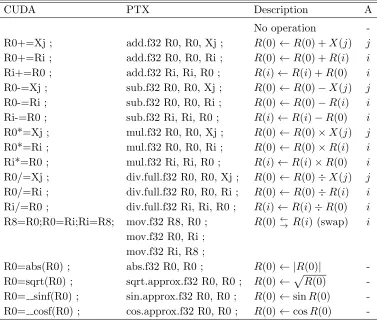
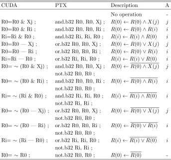
GMGP is capable of evolving linear sequences of single precision floating point operations or linear sequences of Boolean operations. The function set of floating point operations is composed of addition, subtraction, multiplication, division, data transfer, trigonometric, and arithmetic instructions. The function set of Boolean operations is composed of AND, OR, NAND, NOR, and NOT. Table 2 provides the instruction set of the floating point operations, and Table 3 provides the instruction set of the Boolean operations. Each of these instructions has an opcode and one or two arguments. The argument can be a register or memory position. When it is a register, it varies fromR0 toR7. When it is a memory position, it can be used to load input data or a constant value. The maximum number of inputs in GMGP is 256, and the maximum number of predefined constant values is 128. As an example, in Table 4, we present the CUBIN add instruction with all of the variations of its memory positions (X) and the eight auxiliary FPU registers (Ri | i∈[0..7]). Each CUBIN instruction variation with its arguments (constants or registers) has a different hexadecimal.

GMGP addresses only floating point and Boolean operations. Loops and jumps are not handled, as they are not common in the benchmark problems that we consider. However, GMGP could be extended to consider such problems, including mechanisms to restrict jumping to invalid positions and to avoid infinite loops.

Each evolved CUBIN program consists of three segments: header,body, andfooter. The header and footer are the same for all individuals throughout the evolutionary process. They are optimized in the same manner as by the Nvidia compiler. These segments contain the following:

• Header – Loads the evaluation patterns from global memory to registers on the GPU and initializes eight registers with zero.

• Body – The evolved CUBIN code itself.

• Footer – TransfersR0 contents to the global memory, which is the default output of evolved programs, and then executes the exit instruction to terminate the program and return to the evolutionary algorithm main flow.

For each individual, the body of the program is assembled by stacking the hexadecimal code in the same order as the GP tokens have been read. There is no need for comparisons and branches within an individual code because the instructions are executed sequentially. Avoiding comparisons and branches is an important feature of GMGP. As explained before, GPUs are particularly sensitive to conditional branches.

We aggregate all program bodies of the same population into a single GPU kernel. The kernel has only one header and one footer, reducing the size of the population and thus decreasing the time to transfer the program to the GPU memory through the PCIe bus.

6.2 Machine Code Acquisition

(15)

CUDA PTX Description A

No operation -R0+=Xj ; add.f32 R0, R0, Xj ; R(0)←R(0) +X(j) j

R0+=Ri ; add.f32 R0, R0, Ri ; R(0)←R(0) +R(i) i

Ri+=R0 ; add.f32 Ri, Ri, R0 ; R(i)←R(i) +R(0) i

R0-=Xj ; sub.f32 R0, R0, Xj ; R(0)←R(0)−X(j) j

R0-=Ri ; sub.f32 R0, R0, Ri ; R(0)←R(0)−R(i) i

Ri-=R0 ; sub.f32 Ri, Ri, R0 ; R(i)←R(i)−R(0) i

R0*=Xj ; mul.f32 R0, R0, Xj ; R(0)←R(0)×X(j) j

R0*=Ri ; mul.f32 R0, R0, Ri ; R(0)←R(0)×R(i) i

Ri*=R0 ; mul.f32 Ri, Ri, R0 ; R(i)←R(i)×R(0) i

R0/=Xj ; div.full.f32 R0, R0, Xj ; R(0)←R(0)÷X(j) j

R0/=Ri ; div.full.f32 R0, R0, Ri ; R(0)←R(0)÷R(i) i

Ri/=R0 ; div.full.f32 Ri, Ri, R0 ; R(i)←R(i)÷R(0) i

R8=R0;R0=Ri;Ri=R8; mov.f32 R8, R0 ; R(0) ←→R(i) (swap) i mov.f32 R0, Ri ;

mov.f32 Ri, R8 ;

R0=abs(R0) ; abs.f32 R0, R0 ; R(0)← |R(0)| -R0=sqrt(R0) ; sqrt.approx.f32 R0, R0 ; R(0)←p

R(0)

-R0= sinf(R0) ; sin.approx.f32 R0, R0 ; R(0)←sinR(0) -R0= cosf(R0) ; cos.approx.f32 R0, R0 ; R(0)←cosR(0)

-Table 2: Functional description of the single precision floating point instructions. The first column presents the CUDA command; the second presents the PTX instruction; the third describes the action performed; and the fourth column presents the argument for the instruction (jindexes memory positions, andiselects a register). The last two instructions, sinf and cosf, are fast math instructions, which are less accurate but faster versions of sinf and cosf.

Our procedure creates a PTX program containing all of the PTX instructions listed in Tables 2 or 3. In this program, each instruction is embodied inside a loop, where the iteration count at the start of the loop is unknown, which prevents theptxas compiler from removing instructions.

The PTX program is compiled, and the Nvidia cuobjdump tool is used to disassemble the binary code. The disassembled code contains the machine code of all instructions of the PTX program. The challenge is to remove the instructions that belong to each loop control, which is achieved by finding a pattern that repeats along the code. Once the loop controls are removed, each instruction of our instruction set is acquired.

(16)

CUDA PTX Description A

No operation -R0=R0 & Xj ; and.b32 R0, R0, Xj ; R(0)←R(0)∧X(j) j

R0=R0 & Ri ; and.b32 R0, R0, Ri ; R(0)←R(0)∧R(i) i

Ri=Ri & R0 ; and.b32 Ri, Ri, R0 ; R(i)←R(i)∧R(0) i

R0=R0 — Xj ; or.b32 R0, R0, Xj ; R(0)←R(0)∨X(j) j

R0=R0 — Ri ; or.b32 R0, R0, Ri ; R(0)←R(0)∨R(i) i

Ri=Ri — R0 ; or.b32 Ri, Ri, R0 ; R(i)←R(i)∨R(0) i

R0= ∼(R0 & Xj) ; and.b32 R0, R0, Xj ; R(0)←R(0)∧X(j) j

not.b32 R0, R0 ;

R0= ∼(R0 & Ri) ; and.b32 R0, R0, Ri ; R(0)←R(0)∧R(i) i

not.b32 R0, R0 ;

Ri= ∼(Ri & R0) ; and.b32 Ri, Ri, R0 ; R(i)←R(i)∧R(0) i

not.b32 Ri, Ri ;

R0= ∼(R0 — Xj) ; or.b32 R0, R0, Xj ; R(0)←R(0)∨X(j) j

not.b32 R0, R0 ;

R0= ∼(R0 — Ri) ; or.b32 R0, R0, Ri ; R(0)←R(0)∨R(i) i

not.b32 R0, R0 ;

Ri= ∼(Ri — R0) ; or.b32 Ri, Ri, R0 ; R(i)←R(i)∨R(0) i

not.b32 Ri, Ri ;

R0= ∼R0 ; not.b32 R0, R0 ; R(0)←R(0)

-Table 3: Functional description of the Boolean instructions. The first column presents the CUDA command; the second presents the PTX instruction; the third describes the action performed; and the fourth column presents the argument for the instruction (j indexes memory positions, and iselects a register).

The header is the code that comes before the first instruction found, and the footer is the remaining code after the last instruction found.

With the header and footer, our procedure generates a different program to test each instruction acquired. This program contains a header, a footer, and one instruction. The program is executed, and the result is compared to an expected result that was previously computed on the CPU.

6.3 Evaluation Process

(17)

CUBIN (hexadecimal representation) Description A

0x7e, 0x7c, 0x1c, 0x9, 0x0, 0x80, 0xc0, 0xe2, 0x7e, 0x7c, 0x1c, 0xa, 0x0, 0x80, 0xc0, 0xe2, 0x7d, 0x7c, 0x1c, 0x0, 0xfc, 0x81, 0xc0, 0xc2, 0x7d, 0x7c, 0x1c, 0x0, 0x0, 0x82, 0xc0, 0xc2, 0x7d, 0x7c, 0x1c, 0x0, 0x2, 0x82, 0xc0, 0xc2,

0x7d, 0x7c, 0x1c, 0x0, 0x4, 0x82, 0xc0, 0xc2, R(0)←R(0) +X(j) j

0x7d, 0x7c, 0x1c, 0x0, 0x5, 0x82, 0xc0, 0xc2, 0x7d, 0x7c, 0x1c, 0x0, 0x6, 0x82, 0xc0, 0xc2, 0x7d, 0x7c, 0x1c, 0x0, 0x7, 0x82, 0xc0, 0xc2, 0x7d, 0x7c, 0x1c, 0x0, 0x8, 0x82, 0xc0, 0xc2, 0x7d, 0x7c, 0x1c, 0x80, 0x8, 0x82, 0xc0, 0xc2, 0x7e, 0x7c, 0x9c, 0x0f, 0x0, 0x80, 0xc0, 0xe2, 0x7e, 0x7c, 0x1c, 0x0, 0x0, 0x80, 0xc0, 0xe2, 0x7e, 0x7c, 0x1c, 0x3, 0x0, 0x80, 0xc0, 0xe2,

0x7e, 0x7c, 0x9c, 0x3, 0x0, 0x80, 0xc0, 0xe2, R(0)←R(0) +R(i) i

0x7e, 0x7c, 0x1c, 0x4, 0x0, 0x80, 0xc0, 0xe2, 0x7e, 0x7c, 0x9c, 0x4, 0x0, 0x80, 0xc0, 0xe2, 0x7e, 0x7c, 0x1c, 0x5, 0x0, 0x80, 0xc0, 0xe2, 0x7e, 0x7c, 0x9c, 0x5, 0x0, 0x80, 0xc0, 0xe2,

0x7e, 0x7c, 0x9c, 0x0f, 0x0, 0x80, 0xc0, 0xe2, 0x2, 0x7c, 0x1c, 0x0, 0x0, 0x80, 0xc0, 0xe2, 0x1a, 0x7c, 0x1c, 0x3, 0x0, 0x80, 0xc0, 0xe2,

0x1e, 0x7c, 0x9c, 0x3, 0x0, 0x80, 0xc0, 0xe2, R(i)←R(i) +R(0) i 0x22, 0x7c, 0x1c, 0x4, 0x0, 0x80, 0xc0, 0xe2,

0x26, 0x7c, 0x9c, 0x4, 0x0, 0x80, 0xc0, 0xe2, 0x2a, 0x7c, 0x1c, 0x5, 0x0, 0x80, 0xc0, 0xe2, 0x2e, 0x7c, 0x9c, 0x5, 0x0, 0x80, 0xc0, 0xe2,

Table 4: Hexadecimal representation of the add GPU machine code instruction.

parallelization scheme avoids code divergence, as each thread in a block executes the same instruction over a different fitness case, and different individuals are executed by different thread blocks. Therefore, we are employing as much parallelism as possible for a population.

(18)

7. Experiments and Results

In this section, we analyze the performance of GMGP compared with the other GP method-ologies for GPUs. We describe the environment setup, the implementation of the other GP methodologies, the benchmarks, and the analysis of the results obtained from our experi-ments.

7.1 Environment Setup

The GPU used in our experiments was the GeForce GTX TITAN. This processor has 2,688 CUDA cores (at 837 MHz) and 6 GB of RAM (no ECC) with a memory bandwidth of 288.4 GB/s through a 384-bit data bus. The GTX TITAN GPU is based on the Nvidia Kepler architecture, and its theoretical peak performance is characterized by the use of the fused multiply-add (FMA) operations. The GTX TITAN can achieve single precision theoretical peak performance of 4.5 TFLOPs.

GMGP creates the individuals on CPU using a single-threaded code running on a single core of an Intel Xeon CPU X5690 processor, with 32 KB of L1 data cache, 1.5 M of L2 cache, 12 MB of L3 cache, and 24 GB of RAM, running at 3.46 GHz.

The GP methodologies were implemented in C, CUDA 5.5, and PTX 3.2. The compilers used were gcc 4.4.7, nvcc release 5.5, V5.5.0, and ptxas release 5.5, V5.5.0. We had to be careful in setting the compiler optimization level. It is common for the programmer to use a more advanced optimization level to produce a more optimized and faster code. However, the compilation time is a bottleneck for the GP methodologies that require individuals to be compiled. The code generated by the -O2, -O3, and -O4 optimization levels is more opti-mized and executes faster, but more time is spent in the compilation process. Experiments were performed to determine the best optimization level. These experiments indicated that the lowest optimization level, -O0, provided the best results. There were millions of in-dividuals to be compiled, and each individual was executed only once. Accelerating the execution phase was not sufficient to compensate for the time spent optimizing the code during the compilation phase.

We used five widely used GP benchmarks: two symbolic regression problems, Mexican Hat and Salutowicz; one time-series forecasting problem, Mackey-Glass; one image pro-cessing problem, Sobel filter; and one Boolean regression problem, 20-bit Multiplexer. The first four benchmarks were used to evaluate the single precision floating point instructions, whereas the last benchmark was used to evaluate the Boolean instructions. The Mackey-Glass,Boolean Multiplexer, andSobel filterbenchmarks were also used in previous works on GP accelerated by GPUs (Robilliard et al., 2009; Langdon and Banzhaf, 2008c; Langdon, 2010b; Harding and Banzhaf, 2008, 2009). Nevertheless, it is not possible to perform a direct comparison, as they used a different GP model (tree-based GP) and different hardware.

(19)

We used 256 threads per block in our experiments. The block grid is two-dimensional and depends on the number of individuals and the number of fitness cases. For an experi-ment with(number fitness cases, number individuals)the grid is(number fitness cases/256, number individuals).

7.2 GP Implementations

To put the GMGP results in perspective, we compare the performance of GMGP with the other GP methodologies for GPUs: compilation, pseudo-assembly, and interpretation. However, the GP methodologies for GPUs taken from the literature are not based on LGP or inspired algorithms. For this reason, we had to implement an LGP and quantum-inspired approach corresponding to each methodology to make them directly comparable with GMGP. Nevertheless, these implementations are based on the algorithms described in the literature.

The compilation approach is based on the work by Harding and Banzhaf (2009) and is calledCompiler here. The pseudo-assemblyapproach is based on our previous work (Cu-pertino et al., 2011), and is called Pseudo-Assembly here. The interpretation approach is based on the work by Langdon and Banzhaf (2008a) and is called Interpreterhere.

The Compiler and Pseudo-Assembly methodologies use a similar program assembly to the GMGP methodology. The individuals are created by the CPU and sent to the GPU to be computed. The main difference is the assembly of the body of the programs. In Compiler, the bodies are created using CUDA language instructions. When the popula-tion is complete, it is compiled using thenvcc compiler to generate the GPU binary code. In Pseudo-Assembly, the bodies are created using the PTX pseudo-assembly language in-structions. When the population is complete, the code can be compiled with ptxas or the cuModuleLoad C function provided by Nvidia, both of which generate GPU binary code. The Pseudo-Assembly methodology reduces the compilation overhead using the JIT com-pilation.

In the Interpreter methodology, the interpreter was written in the PTX language, rather than in RapidMind, as proposed by Langdon and Banzhaf (2008a). The interpreter is au-tomatically built once, at the beginning of the GP evolution, and is reused to evaluate all individuals. Algorithm 1 presents a high-level description of the interpreter process. As the pseudo-assembly language does not have a switch-case statement, we used a combina-tion of the instruccombina-tion setp.eq.s32(comparisons) andbra (branches) to obtain the same functionality. These comparisons and branches represent one of the weaknesses of the In-terpreter methodology. The inIn-terpreter must execute more instructions than the actual GP operations. For each GP instruction, we have at least one comparison, to identify the GP operation, and one jump to the beginning of the loop. In addition, comparisons can be made to identify the instruction arguments.

(20)

1: TBX←X dimension of the Thread Block identification 2: TBY←Y dimension of the Thread Block identification

3: INDIV←individual number (TBY)

4: N←program length (INDIV)

5: THREAD←GPU Thread identification

6: X0←input variable 1 (THREAD + TBX * Number of threads in a block) 7: X1←input variable 2 (THREAD + TBX * Number of threads in a block) 8: fork←1toN do

9: INSTRUCT←instruction number (k) (INDIV)

10: ARG←argument number (k) (INDIV)

11: switch(INSTRUCT)

12: case0: 13: no operation 14: case1:

15: switch(ARG) % Description: R(0)←R(0) +X(j)

16: case0:

17: add.f32 R0, R0, X0 18: case1:

19: add.f32 R0, R0, X1

20: →Here, we have more similar cases for all inputs and constant registers (X).

21: end switch

22: case2:

23: switch(ARG) % Description: R(0)←R(0) +R(i)

24: case0:

25: add.f32 R0, R0, R0 26: case1:

27: add.f32 R0, R0, R1

28: →Here, we have more similar cases for all eight auxiliary FPU registers (Ri).

29: end switch

30: case3:

31: switch(ARG) % Description: R(i)←R(i) +R(0)

32: case0:

33: add.f32 Ri, R0, R0 34: case1:

35: add.f32 Ri, R1, R0

36: →Here, we have more similar cases for all eight auxiliary FPU registers (Ri).

37: end switch

38: →Here, we have more similar cases for all other instructions, such as subtraction, multiplication, division, data transfer, trigonometric, and arithmetic operations.

39: default:

40: exit

41: end switch

42: →Write result back to global memory.

43: end for

(21)

7.3 Symbolic Regression Benchmarks

Symbolic regression is a typical problem used to assess GP performance. We used two well-known benchmarks: the Mexican Hat and Salutowicz. These benchmarks allow us to evaluate GMGP over different fitness case sizes.

The Mexican Hat benchmark (Brameier and Banzhaf, 2007) is represented by a two-dimensional function given by Equation (8):

f(x,y) =

1−x

2 4 −

y2

4

×e(−x2−y2)/8. (8) The Salutowicz benchmark (Vladislavleva et al., 2009) is represented by Equation (9). We used the two-dimensional version of this benchmark.

f(x,y) = (y−5)×e−x×x3×cos(x)×sin(x)×hcos(x)×sin(x)2−1

i

. (9)

For the Mexican Hat benchmark, the x and y variables are uniformly sampled in the range [−4,4]. For the Salutowicz benchmark, they are uniformly sampled in the range [0,10]. This sampling generates the training, validation, and testing data sets. The number of subdivisions of each variable can be 16, 32, 64, 128, 256, and 512, which is called the number of samples, N. At each time, both variables use the same value ofN, producing a grid. WhenN = 16, there is a 16×16 grid, which represents 256 fitness cases. Accordingly, the number of fitness cases varies in the set S={256, 1024, 4096, 16K, 64K, 256K}.

These two benchmarks represent two different surfaces, and GP has the task of recon-structing these surfaces from a given set of points. The fitness value of an individual is its mean absolute error (MAE) over the training cases, as given by Equation (10):

MAE = 1

n n X

i=1

|t_i−V[0]i|, (10)

whereti is the target value for the ithcase andV[0]i is the individual output value for the

same case.

7.3.1 Parameter Settings

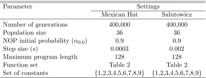
Table 5 presents the parameters used when executing the Mexican Hat and Salutowicz benchmarks. We used a small population size, which is a typical characteristic of QEAs. The evolution status of QEAs is represented by a probability distribution, and there is no need to include many individuals. The superposition of states provides a good global search ability due to the diversity provided by the probabilistic representation.

7.3.2 Preliminary Experiments for the Compiler Methodology

(22)

Parameter Settings

Mexican Hat Salutowicz

Number of generations 400,000 400,000

Population size 36 36

NOP initial probability (α0,0) 0.9 0.9

Step size (s) 0.0003 0.002

Maximum program length 128 128

Function set Table 2 Table 2

Set of constants {1,2,3,4,5,6,7,8,9} {1,2,3,4,5,6,7,8,9}

Table 5: Parameter settings for the Mexican Hat and Salutowicz benchmarks. The values of number of generations, population size, initial probability of NOP, and step size were obtained from previous experiments.

Methodology Total nvcc upload evaluation interpret download CPU

GMGP 292.6 – 73.2 76.9 – 5.13 137.2

Interpreter 636.8 – 3.14 – 542.4 4.35 86.8

Pseudo-Assembly 40,777 – 40,414 118.8 – 6.13 238.8

Compiler 242,186.7 135,027.5 106,458 283.6 – 6.74 410.9

Table 6: Execution time breakdown of all GPU methodologies (in seconds). The table presents the times for: Total, the total execution; nvcc, the compilation in the nvcc compiler;upload, the compilation of the PTX code (Compiler and Pseudo-Assembly), or loading the GPU binaries to the GPU memory (GMGP), or transfer-ring the tokens through the PCIe bus (Interpreter);evaluation, the computation of the fitness cases;interpret, the interpretation;download, the copy of the fit-ness result from GPU to the CPU; andCPU, the GP methodology is executed on the CPU.

the GPU binaries to the graphic card before execution); in the interpreter methodology,

upload is the time necessary to transfer the tokens through the PCIe bus; evaluation

represents the time spent computing the fitness cases;interpretis the interpretation time for Interpreter; download is the time spent in copying the fitness result from GPU to the CPU; andCPUrepresents the remainder of the execution time, including the time necessary to execute the GP methodology on the CPU.

(23)

Banzhaf (2007) and Chitty (2007) did not use CUDA and could therefore avoid the nvcc overhead. Harding and Banzhaf (2009) used CUDA but handled the compilation overhead by using a cluster to compile the population. Langdon and Harman (2010) also used CUDA, but the total compilation time for our experiment is greater than their compilation time for two reasons. First, the small population size of a quantum-inspired approach requires more compiler calls. Second, the total number of individuals we are evaluating (number of generations × population size) is at least one order of magnitude greater than in their experiments.

Because the other methodologies solved the same problem considerably faster, we dis-carded the Compiler methodology for the remaining experiments.

Thedownloadtime is almost the same for all implementations because the same data set was used in all approaches. Accordingly, the results to be copied through the PCIe bus are the same. The CPU time for Interpreter is slightly smaller than for GMGP, Compiler, and Pseudo-Assembly because Interpreter does not have to assemble the individuals in the CPU before transferring to the GPU. Instead, the tokens are copied directly. The evaluation

time is almost the same for Compiler and Pseudo-Assembly, but GMGP presents a slightly smaller evaluation time because the header and footer are optimized. The interpret

time is approximately one order of magnitude slower than the GMGP evaluation time because it has to perform many additional instructions, such as comparisons and jumps. The upload time for GMGP is approximately three orders of magnitude faster than the

upload time for Compiler and Pseudo-Assembly because GMGP directly assembles the GPU binaries without calling the PTX compiler. The time necessary to transfer the tokens through the PCIe bus in the Interpreter methodology is smaller than the time necessary to load the GPU binary code in the GMGP.

7.3.3 Performance Analysis

We compare the execution times of the methodologies as the number of fitness cases varies in the set: S={256, 1024, 4096, 16K, 64K, 256K}. The total execution times of theMexican HatandSalutowiczbenchmarks for the Pseudo-Assembly, Interpreter, and GMGP method-ologies are presented in Figure 5. The curves are plotted in log-scale. The Pseudo-Assembly methodology execution time remains almost constant as the problem size increases in both cases studied because Pseudo-Assembly spends most of the time compiling the individual population code, and the compilation time does not depend on the problem size. The total execution times of the Interpreter and GMGP methodologies increase almost linearly as the number of fitness cases increases from 256 to 256K. For the largest data set, 256K, the Pseudo-Assembly execution time approaches the execution time of Interpreter. How-ever, the Pseudo-Assembly methodology performs much worse than the other methodologies when only a few fitness cases are considered.

(24)

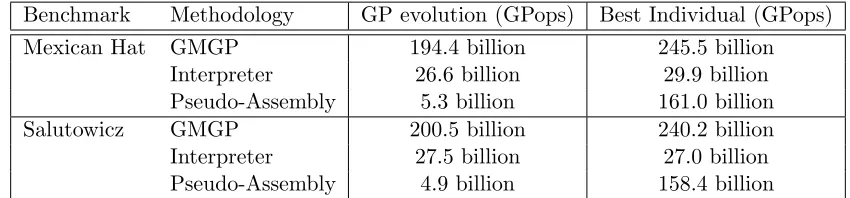
Benchmark Methodology GP evolution (GPops) Best Individual (GPops) Mexican Hat GMGP 194.4 billion 245.5 billion

Interpreter 26.6 billion 29.9 billion Pseudo-Assembly 5.3 billion 161.0 billion Salutowicz GMGP 200.5 billion 240.2 billion Interpreter 27.5 billion 27.0 billion Pseudo-Assembly 4.9 billion 158.4 billion

Table 7: Performance of GMGP, Interpreter, and Pseudo-Assembly for Mexican Hat and Salutowicz in GPops. The table presents the results for the overall evolution, including the time spent in the GPU and CPU, and the results for the GPU computation of the best individual after the evolution is complete.

Figure 5: Execution time (in seconds) of Pseudo-Assembly, Interpreter, and GMGP methodologies for theMexican HatandSalutowiczbenchmarks with an increasing number of fitness cases.

methodology had the smallest values, 5.3 billion GPops for Mexican Hat and 4.9 billion GPops forSalutowicz. Table 7 also presents the GPops for the evaluation in the GPU of the best individual found after the evolution is completed. The best individual GPops results are greater than the GP evolution results because the evaluation of the best individual takes considerably less time than the whole GP evolution. In addition, the GP evolution includes the overheads of creating the individuals and transferring the data to/from the GPU. For Pseudo-Assembly, the evaluation of the best individual does not consider the compilation overhead, and the GPops value obtained for the best individual is similar to that obtained by GMGP.

(25)

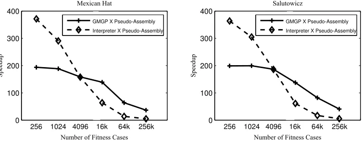
Figure 6: Speedup of Interpreter and GMGP compared to Pseudo-Assembly for theMexican Hatand Salutowicz benchmarks with an increasing number of fitness cases.

Mexican Hat, Interpreter runs 371 times faster than Pseudo-Assembly, whereas GMGP runs 193 times faster than Pseudo-Assembly. The gains are similar for Salutowicz: In-terpreter runs 363 times faster than Pseudo-Assembly, and GMGP runs 199 times faster than Assembly. As the problem size increases, the speedups compared to Pseudo-Assembly become smaller for both benchmarks. We will compare only Interpreter and GMGP in the remainder of this analysis.

Figure 7 presents the speedup obtained with GMGP compared to Interpreter forMexican Hat and Salutowicz. GMGP performs better for larger data sets for both benchmarks. For the small data sets, in GMGP, the number of fitness cases used is not sufficient to compensate for the overhead of uploading the individuals, and the Interpreter methodology is faster. GMGP outperforms Interpreter for fitness case sizes exceeding 4,096. GMGP is 7.3 times faster than Interpreter for Mexican Hat and a fitness case size of 256K. Similar results were obtained for Salutowicz. As expected, GMGP is promising for applications with large data sets.

To explain why GMGP outperforms Interpreter for large data sets, we analyze the execution time breakdown for each approach in detail. Figures 8 and 9 present the execution breakdown of GMGP and Interpreter for the Mexican Hat and Salutowicz benchmarks with an increasing number of fitness cases. The execution time was broken into the same components as described in Table 6.

(26)

Figure 7: Speedup of GMGP compared to Interpreter for theMexican Hat and Salutowicz benchmarks with an increasing number of fitness cases.

256 1024 4096 16k 64k 256k 0

200 400 600 800 1000

Number of Fitness Cases

A

verage

T

ime (seconds)

Mexican Hat − GMGP

upload evaluation download CPU

256 1024 4096 16k 64k 256k

0 200 400 600 800 1000

A

verage

T

ime (seconds)

Salutowicz − GMGP

upload evaluation download CPU

Figure 8: Execution time breakdown of GMGP. The graph presents the time broken down as follows: upload, the time spent loading the GPU binaries to the GPU memory; evaluation, the time spent computing the fitness cases; download, the time spent copying the fitness result from the GPU to the CPU; and CPU, the time during which the GP methodology is executed on the CPU.

(27)

256 1024 4096 16k 64k 256k 0 200 400 600 800 1000

A

verage

T

ime (seconds)

Mexican Hat − Interpreter

2127 seconds 8484 seconds upload interpret download CPU

256 1024 4096 16k 64k 256k

0 200 400 600 800 1000

A

verage

T

ime (seconds)

Salutowicz − Interpreter

2198 seconds 8892 seconds upload interpret download CPU

Figure 9: Execution time breakdown of Interpreter. The graph presents the time broken into: upload, the time necessary to transfer the tokens through the PCIe bus; interpret, the interpretation time; download, the time spent copying the fitness result from the GPU to the CPU; and CPU, the time during which the GP methodology is executed on the CPU.

evaluation function times for GMGP and Interpreter by comparing theevaluationtime of Figure 8 with the interpret time of Figure 9. For small data sets, the evaluation time of GMGP is smaller than the interpret time of Interpreter, but the difference is small. However, as the problem size increases, theinterpret time increases significantly because the Interpreter methodology must execute an excessive amount of additional instructions, such as comparisons and branches. For GMGP, the evaluation time increases slightly because it executes only the necessary GP instructions. Thus, the total time difference between GMGP and Interpreter increases for larger data sets.

7.3.4 Quality of Results

To compare the quality of the results of the Compiler, Pseudo-Assembly, Interpreter, and GMGP methodologies on the GPU, we used the same random seed at the beginning of the first experiment of each approach. We compared the intermediate and final results. All GPU approaches produced identical results, comparing all available precision digits. The only difference among them was the execution time.

(28)

Benchmark Methodology Training Validation Test Average σ Average σ Average σ

Mexican Hat GMGP 0.046 0.007 0.048 0.008 0.053 0.008 Interpreter 0.046 0.007 0.048 0.008 0.053 0.008 Pseudo-Assembly 0.046 0.007 0.048 0.008 0.053 0.008 Compiler 0.046 0.007 0.048 0.008 0.053 0.008 Salutowicz GMGP 0.17 0.10 0.19 0.12 0.15 0.08

Interpreter 0.17 0.10 0.19 0.12 0.15 0.08 Pseudo-Assembly 0.17 0.10 0.19 0.12 0.15 0.08 Compiler 0.17 0.10 0.19 0.12 0.15 0.08

Table 8: Mean Absolute Errors (MAEs) in GPU evolution for the Mexican Hat and Salu-towiczbenchmarks. The table presents the best individuals’ average and standard deviation (σ) for the training, validation, and testing data sets for 16K fitness cases, with a precision of 10−3.

7.4 Mackey-Glass Benchmark

The Mackey-Glass benchmark (Jang and Sun, 1993) is a chaotic time-series prediction benchmark, and the Mackey-Glass chaotic system is given by the non-linear time delay differential Equation (11).

dx(t)

dt =

0.2x(t−τ)

1 +x10₍_t₋_τ₎ −0.1x(t) (11) TheMackey-Glasssystem has been used as a GP benchmark in various works (Langdon and Banzhaf, 2008b,c). In our experiments, the time series consists of 1,200 data points, and GP has the task of predicting the next value when historical data are provided. The GP inputs are eight earlier values from the series, at 1, 2, 4, 8, 16, 32, 64, and 128 time steps ago.

The parameters used for the GP evolution in theMackey-Glassbenchmark are presented in Table 9. We used a small population size and a large number of generations, as previously explained. The number of generations was defined according to the number of individuals proposed by Langdon and Banzhaf (2008c).

(29)

Parameter Settings

Number of generations 512,000

Population size 20

NOP initial probability (α0,0) 0.9

Step size (s) 0.004

Maximum program length 128

Function set Table 2

Set of constants {0,0.01,0.02, ..., 1.27}

Table 9: Parameter settings for the Mackey-Glass benchmark. The number of individuals (number of population x number of generations) was defined according to the literature. The initial probability of NOP and step size were obtained in previous experiments.

GPops

GP evolution 77.7 billion + loading data 8.85 billion + results transfer 8.4 billion Total computation 3.59 billion Best individual 8.6 billion

Table 10: Results of GMGP running the Mackey-Glass benchmark in GPops. The table presents the number of GPops spent in the GP evolution in the GPU, progres-sively including the overhead of loading the individuals code into GPU and trans-ferring the results back to the CPU. At the end, we provide the results for the entire computation, including the overhead of CPU computation, and the results for the execution of the best individual.

individual code into the GPU memory, GMGP obtained 8.85 billion GPops. The load of data into the GPU memory does not include any GP operation and requires a substantial time in the evolution process. The load time is fixed regardless of the size of the data set. The idea is to amortize this cost by the faster execution of a larger data set. However, the Mackey-Glassbenchmark has a small number of fitness cases.

(30)

Figure 10: The three gray-scale images used for training. The image resolutions are 512×

512 pixels.

7.4.3 Quality of the Results

The quality of the results produced by GMGP was analyzed using 10 GP executions. We computed the RMS error and standard deviation. The average error was 0.0077, and the standard deviation was 0.0021. The error is lower than the errors presented in the literature due to the difference in the GP models used. The results presented in the literature used a tree-based GP with a tree size limited to 15 and depth limited to 4. In contrast, GMGP can evolve individuals with at most 128 linear instructions. Accordingly, it was possible to find an individual that better addressed this benchmark problem.

7.5 Sobel filter

The Sobel filter is a widely used edge detection filter. Edges characterize boundaries and are therefore considered crucial in image processing. The detection of edges can assist in image segmentation, data compression, and image reconstruction. The Sobel operator calculates the approximate image gradient of each pixel by convolving the image with a pair of 3×3 filters. These filters estimate the gradients in the horizontal (x) and vertical (y) directions, and the magnitude of the gradient is the sum of these gradients. All edges in the original image are greatly enhanced in the resulting image, and the slowly varying contrast is suppressed.

(31)

Figure 11: The two gray-scale images used for validation. The image resolutions are 512×

512 pixels.

Figure 12: Results of evolving the filter for one test image. The leftmost image is the original gray-scale test image. The center image is the output image produced by applying the GIMP Sobel filter. The rightmost image is the output image produced by the GMGP evolved filter.

The parameters used for the GP evolution of theSobel filter are presented in Table 11. The population size also employs a low number of individuals for the reasons explained before. The number of generations, NOP initial probability, step size, and maximum program length were obtained from previous experiments.

(32)

Parameter Settings

Number of generations 400,000

Population size 20

Step size (s) 0.001

Set of constants {1,2,3,4,5,6,7,8,9}

Table 11: Parameter settings for the Sobel filter. The values of the number of generations, population size, initial probability of NOP, and step size were obtained in previous experiments.

GPops

GP evolution 287.3 billion + loading data 274.2 billion + results transfer 268.6 billion Total computation 249.9 billion Best individual 295.8 billion

Table 12: Results of GMGP running the Sobel filter in GPops. The table presents the number of GPops spent in the GP evolution in the GPU, progressively including the overheads of loading the individual code into the GPU and transferring the results back to the CPU. At the end, we present the results for the entire com-putation, including the overhead of CPU comcom-putation, and the results for the execution of the best individual.

of transferring the results back to the CPU through the PCIe bus, GMGP obtained 268.6 billion GPops. When the entire computation is considered, including the overhead of the CPU computation during the evolution, GMGP obtained 249.9 billion GPops. After the evolution, the best individual was executed on the GPU, and we calculated a performance of 295.8 billion GPops for the best individual.

(33)

Training Validation Test Average σ Average σ Average σ

2.11 0.61 2.21 0.64 2.03 0.599

Table 13: MAEs in GMGP evolution for the Sobel filter. The table presents the average and standard deviation (σ) of the best individual for the training, validation, and testing data sets.

best individual of GMGP applied to the test image. This image can be visually compared to the image in the center of Figure 12, which was obtained using theSobel filter of GIMP. A visual comparison of these two images indicates that the evolved filter produced an image with more prominent horizontal edges without significantly increasing the noise.

7.6 20-bit Boolean Multiplexer

The Boolean instructions of GMGP were evaluated using the 20-bit Boolean Multiplexer benchmark (Langdon, 2010b, 2011). In the20-bit Boolean Multiplexerbenchmark, there are 1,048,576 possible combinations of 20 arguments of a 20-bit Multiplexer. In our experiments, we used 1,048,576 fitness cases to evaluate all of the individuals, which is possible because GMGP evaluates each individual rapidly. This experiment is the first time this benchmark has been solved in this manner, using all fitness cases. The bit-level parallelism was exploited by performing bitwise operations over a 32-bit integer that packs 32 Boolean fitness cases.

The parameter settings used for the 20-bit Boolean Multiplexer benchmark are presented in Table 14. More individuals were used in the population than in the previous benchmark experiments reported in this paper. This problem addresses more input variables and a larger data set. The number of generations was computed to produce a total number of individuals similar to the numbers presented in the literature. However, the zero error solution was found before the maximum number of generations was reached for all 10 GP executions. The maximum program length was obtained by verifying the minimum length needed to solve this problem benchmark.

Table 15 presents the number of GPops obtained by GMGP for the GP evolution in the GPU (execution of the evaluation of all individuals considering the non-NOP operations); the GP evolution including the loading of the individual code into the GPU memory; the GP evolution, including the loading of the individuals and the transfer of the results to the CPU memory; the total computation, including the CPU computation; and the best individual computation.

(34)

Parameter Settings

Number of generations First Solution or 14,000,000

Population size 40

Step size (s) 0.004

Set of constants –

Table 14: Parameter settings for the20-bit Boolean Multiplexer. The values of the number of generations, population size, initial probability of NOP, and maximum program length were obtained in previous experiments, where we varied the values until the problem was solved.

GPops GP evolution 5.88 trillion + loading data 5.24 trillion + results transfer 5.19 trillion Total computation 2.74 trillion Best individual 4.87 trillion

Table 15: Results of GMGP running the 20-bit Boolean Multiplexerbenchmark in GPops. The table presents the number of GPops spent in the GP evolution in the GPU, progressively including the overhead of loading the individual code into GPU and transferring the results back to the CPU. At the end, we present the results for the entire computation, including the overhead of CPU computation, and the results for the execution of the best individual.

(35)

Experiment Generation Total Number of Individuals

1 2,413,505 96,540,200

2 1,246,979 49,879,160

3 3,238,394 129,535,760

4 7,802,509 312,100,360

5 8,892,873 355,714,920

6 10,737,990 429,519,600

7 5,255,728 210,229,120

8 2,576,655 103,066,200

9 5,469,381 218,775,240

10 3,395,730 135,829,200

Table 16: Generation at which GMGP solved the20-bit Boolean Multiplexer and the total number of individuals used in the evolution. The population size is 40 individuals.

GMGP was able find the zero solution for the20-bit Boolean Multiplexerbenchmark before the maximum number of generations was reached for all 10 GP executions. Table 16 presents the number of generations and total number of individuals needed to find this solution.

8. Discussions