Multi-scale Classification using Localized Spatial Depth
Subhajit Dutta [email protected]
Department of Mathematics and Statistics Indian Institute of Technology
Kanpur 208016, India.
Soham Sarkar [email protected]
Anil K. Ghosh [email protected]
Theoretical Statistics and Mathematics Unit Indian Statistical Institute
203, B. T. Road, Kolkata 700108, India.
Editor:Jie Peng
Abstract
In this article, we develop and investigate a new classifier based on features extracted using spatial depth. Our construction is based on fitting a generalized additive model to posterior probabilities of different competing classes. To cope with possible multi-modal as well as non-elliptic nature of the population distribution, we also develop a localized version of spatial depth and use that with varying degrees of localization to build the classifier. Final classification is done by aggregating several posterior probability estimates, each of which is obtained using this localized spatial depth with a fixed scale of localization. The proposed classifier can be conveniently used even when the dimension of the data is larger than the sample size, and its good discriminatory power for such data has been established using theoretical as well as numerical results.
Keywords: Bayes classifier, elliptic distributions, generalized additive models, HDLSS asymptotics, uniform strong consistency, weighted aggregation of posteriors.
1. Introduction
In a supervised classification problem with J competing classes, we have nj labeled obser-vationsxj1, . . . ,xjnj from thej-th class (1≤j≤J). We use this training sample consisting
of n = PJ
−10 −5 0 5 10
−10
−5
0
5
10
X1 X2
−10 −5 0 5 10
−10
−5
0
5
10
X1 X2
(a) ExampleE1
−4 −2 0 2 4
−4
−2
0
2
4
X1 X2
−4 −2 0 2 4
−4
−2
0
2
4
X1 X2
(b) ExampleE2
Figure 1: Bayes class boundaries inR2.
density estimates (KDE) (see, e.g., Scott, 2015) are more flexible and free from such model assumptions. But, they suffer from the curse of dimensionality and are often not suitable for high-dimensional data.
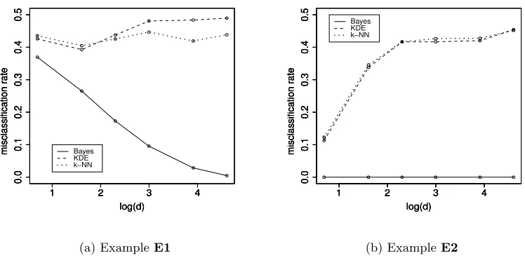
To demonstrate this, let us consider two examples denoted by E1andE2. E1involves a classification problem with two classes in Rd, where the distribution of the first class is
an equal mixture of Nd(0d,Id) and Nd(0d,10Id), and that of the second class is Nd(0d,5Id). Here Nddenotes thed-variate normal distribution,0d= (0, . . . ,0)T ∈RdandIdis thed×d identity matrix. InE2, each class distribution is an equal mixture of two uniform distribu-tions. For the first (respectively, the second) class, it is a mixture of Ud(0,1) and Ud(2,3) (respectively, Ud(1,2) and Ud(3,4)), where Ud(r1, r2) denotes the uniform distribution over the region {x∈Rd :r
1 ≤ kxk ≤ r2} with 0 ≤r1 < r2 <∞ and k · kbeing the Euclidean norm. Figure 1 shows the class boundaries of the Bayes classifier for these two examples when d= 2 and π1 =π2 = 1/2. The regions colored grey (respectively, black) correspond to observations classified to the first (respectively, the second) class by the Bayes classifier. It is clear that classifiers like LDA and QDA, or any other classifier with linear or quadratic class boundaries will deviate significantly from the Bayes classifier in both examples. A natural question then is how standard nonparametric classifiers like those based on k-NN and KDE perform in such examples.
1 2 3 4
0.0
0.1
0.2
0.3
0.4
0.5
log(d)
misclassification r
ate
1 2 3 4
0.0
0.1
0.2
0.3
0.4
0.5
log(d)
misclassification r
ate
1 2 3 4
0.0
0.1
0.2
0.3
0.4
0.5
log(d)
misclassification r
ate
Bayes KDE k−NN
(a) ExampleE1
1 2 3 4
0.0
0.1
0.2
0.3
0.4
0.5
log(d)
misclassification r
ate
1 2 3 4
0.0
0.1
0.2
0.3
0.4
0.5
log(d)
misclassification r
ate
1 2 3 4
0.0
0.1
0.2
0.3
0.4
0.5
log(d)
misclassification r
ate
Bayes KDE k−NN
(b) ExampleE2
Figure 2: Average misclassification rates of nonparametric classifiers and the Bayes classifier ford= 2,5,10,20,50 and 100.
These two examples clearly show the necessity to develop new classifiers to cope with such situations. We use the idea of data depth for this purpose. Over the last three decades, data depth (see, e.g., Liu et al., 1999; Zuo and Serfling, 2000) has emerged as a powerful tool for multivariate data analysis with applications in many areas including supervised and unsupervised classification (see, e.g., Jornsten, 2004; Ghosh and Chaudhuri, 2005a,b; Hoberg and Mosler, 2006; Xia et al., 2008; Dutta and Ghosh, 2012; Li et al., 2012; Lange et al., 2014; Paindaveine and Van Bever, 2015). Spatial depth (also known as theL1 depth) is a popular notion of data depth that was introduced and studied by Vardi and Zhang (2000) and Serfling (2002). Thespatial depth(SPD) of an observationx∈Rdwith respect to (w.r.t.) a distribution functionF onRdis defined as SPD(x, F) = 1−EF[u(x−X)]
,where
X∼F, andu(·) is the multivariate sign function given by u(x) =kxk−1xifx6=0d ∈Rd,
and u(0d) = 0d. This version of SPD is invariant w.r.t. location shift, orthogonal, and homogeneous scale transformations. SPD is often computed on the standardized version of
X as well. In that case, it is defined as SPD(x, F) = 1−
EF[u(Σ−1/2(x−X))]
,
where Σ is a scatter matrix associated with F. One can check that if Σ has the affine equivariance property (see, e.g., Zuo and Serfling, 2000), this version of SPD is affine in-variant. To differentiate between these two versions of SPD, we will denote them by SPD◦ and SPD∗, respectively. IfΣ=λId for someλ >0 (e.g., if F is spherically symmetric, see Fang et al., 1990), then SPD◦ and SPD∗ coincide. Throughout this article, the term SPD will be used in a generic sense.
pair of probability distributions F1 and F2, if SPD(x, F1) is larger than SPD(x, F2), one would expect x to come from F1 instead of F2. Based on this simple idea, the maximum
depth classifier was developed by Jornsten (2004); Ghosh and Chaudhuri (2005b). For a
J class problem involving distributionsF1, . . . , FJ, the maximum depth classifier based on SPD assigns an observation xto thej0-th class, where j0 = argmax1≤j≤JSPD(x, Fj).
0 2 4 6 8 10
0.0
0.2
0.4
0.6
0.8
1.0
||x||
SPD
SPD(x, F1)
SPD(x, F2)
(a) ExampleE1
0 1 2 3 4 5
0.0
0.2
0.4
0.6
0.8
1.0
||x||
SPD
SPD(x, F1)
SPD(x, F2)
(b) ExampleE2
Figure 3: SPD(x, F1) and SPD(x, F2) for different values of kxk when x∈R2.
In E1 and E2, since the class distributions are spherically symmetric, SPD∗ coincides with SPD◦, and they become a monotonically decreasing function of the Euclidean norm of x(see Lemma 7). In Figure 3, we have plotted SPD(x, F1) and SPD(x, F2) for different values of kxk in E1and E2, where F1 and F2 are the distributions of the two classes and
x∈R2. It is transparent from Figure 3 that the maximum depth classifier based on SPD
will fail in both examples. InE1, for all values ofkxksmaller (respectively, greater) than a constant close to 4, the observations will be classified to the first (respectively, the second) class by the maximum SPD classifier. On the other hand, this classifier will classify all observations to the second class in E2. Most of the popular depth functions turn out to be monotonically decreasing functions of the Euclidean norm in the case of a spherically symmetric distribution. So, the maximum depth classifiers based on those depth functions will have similar problems as well.
Almost all existing depth based classifiers require ellipticity of class distributions to achieve Bayes optimality. To cope with possible multi-modal as well as non-elliptic popu-lation distributions, we construct a localized version of spatial depth (LSPD) in Section 3. In Section 4, we develop a multi-scale classifier based on LSPD. Relevant theoretical results on SPD, LSPD and the resulting classifiers are studied in these sections. In Sections 5 and 6, some simulated and benchmark data sets are analyzed to demonstrate the usefulness of these proposed classifiers. An advantage of SPD over other depth functions is its compu-tational simplicity. Classifiers based on SPD and LSPD can be constructed even when the dimension exceeds the sample size. We deal with such high dimension, low sample size (HDLSS) cases in Section 7, and show that both classifiers turn out to be optimal under a fairly general framework. Several high-dimensional data sets are also analyzed to evaluate their empirical performance. All proofs and mathematical details are given in Appendix A.
2. Bayes Optimality of a Classifier Based on Spatial Depth
Let us assume thatf1, . . . , fJ are density functions ofJ elliptically symmetric distributions (Fang et al., 1990) on Rd, where fj(x) = |Σj|−1/2gj(kΣ
−1/2
j (x−µj)k) for 1 ≤ j ≤ J. Here µj ∈ Rd, Σ
j is a d×d symmetric and positive definite matrix, and gj(ktk) is a probability density function of a spherically symmetric distribution on Rd for 1 ≤ j ≤ J.
For such classification problems involving general elliptic populations with equal or unequal priors, the next theorem establishes the Bayes optimality of a classifier, which is based on
z∗(x) = (z1∗(x), . . . , zJ∗(x))T = (SPD∗(x, F1), . . . ,SPD∗(x, FJ))T.
Theorem 1 If the densities ofJ competing classes are elliptically symmetric, the posterior probabilities of these classes satisfy the logistic regression model given by
p(j|x) = ˜p(j|z∗(x)) = exp(Φj(z ∗(x))) [1 +P(J−1)
k=1 exp(Φk(z∗(x)))]
for 1≤j ≤(J −1) (1)
and p(J|x) = ˜p(J|z∗(x)) = 1 [1 +P(J−1)
k=1 exp(Φk(z∗(x)))]
. (2)
Here Φj(z∗(x)) =ϕj1(z∗1(x)) +· · ·+ϕjJ(zJ∗(x)), andϕjis are appropriate real-valued
func-tions ofπj and fj for 1≤j≤J. Consequently, the Bayes rule assigns an observation xto
the classj0, where j0 = argmax1≤j≤J p˜(j|z∗(x)).
Theorem 1 shows that the Bayes classifier is based on a nonparametric multinomial additive logistic regression model for the posterior probabilities, which is a special case of generalized additive models (GAM) (Hastie and Tibshirani, 1990). If the prior probabilities of J classes are equal, and f1, . . . , fJ are all elliptic and unimodal differing only in their locations, this Bayes classifier reduces to the maximum depth classifier (Ghosh and Chaud-huri, 2005b) (see Remark 8 after the proof of Theorem 1 in Appendix A). A special case of Theorem 1 withΣj =λjId, whereλj >0 for 1≤j≤J is stated below.
Corollary 2 If the densities ofJ competing classes are spherically symmetric (i.e.,fj(x) =
gj(kx−µjk) for 1 ≤ j ≤ J), then the posterior probabilities of these classes satisfy the
For any fixediandj, one can calculate theJ-dimensional vectorz◦(xji) (or,z∗(xji)), where
xji is the i-th labeled observation from thej-th class for 1≤i≤nj and 1≤j≤J. These
z◦(xji)s (or, z∗(xji)s) can be viewed as realizations of the vector of covariates in a non-parametric multinomial additive logistic regression model, where the response corresponds to the class label that belongs to {1, . . . , J}. Now, a classifier based on SPD can be con-structed by fitting a GAM with the logistic link function. This procedure can be viewed as a multinomial logistic regression in the J-dimensional depth plot. Lange et al. (2014); Li et al. (2012); Mozharovskyi et al. (2015) used such plots for nonparametric classification. Recently, Cuesta-Albertos et al. also considered GAM to construct a depth based classifier for functional data. In practice, we use a random sample x1, . . . ,xn generated fromF to compute the empirical versions of SPD◦ and SPD∗, which are given by
SPD◦(x, Fn) = 1−
1
n
n
X
i=1
u(x−xi)
and SPD∗(x, Fn) = 1−
1
n
n
X
i=1
u(Σb
−1/2
(x−xi))
,
respectively, where Σb is an estimate of Σ, andFn is the empirical distribution of the data
x1, . . . ,xn. Clearly, SPD∗ is affine invariant ifΣb has the affine equivariance property. The
resulting classifier worked quite well in examplesE1andE2, and we shall see the numerical results later in Section 5.1.
3. Extraction of Small Scale Distributional Features by Localization of Spatial Depth
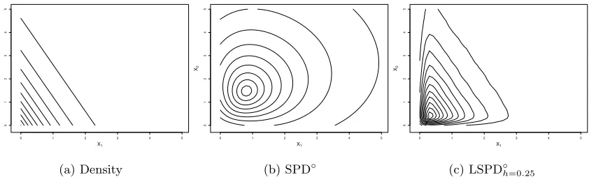
Under elliptic symmetry, the density function of a class can be expressed as a function of SPD∗, and hence the depth contours coincide with the density contours. This is the main mathematical argument used in the proof of Theorem 1. For non-elliptic distributions, where the density function cannot be expressed as a function of SPD, such mathematical arguments are no longer valid. Consider an equal mixture of Nd(0d,0.25Id), Nd(21d,0.25Id) and Nd(41d,0.25Id), where1d= (1, . . . ,1)T denotes ad-dimensional vector with all elements equal to 1. We have plotted the density contours in Figure 4(a) and SPD◦ contours in Figure 4(b) when d= 2. In this trimodal distribution, the SPD◦ contours failed to match the density contours. As a second example, we consider a d-dimensional distribution with independent components, where thei-th component is exponential with the scale parameter
d/(d−i+ 1) for 1≤i≤d. Figures 5(a) and 5(b) show the density contours and the SPD◦ contours, respectively, when d = 2. Even in this example, SPD◦ and density contours differed significantly. We observed a similar picture for contours based on SPD∗ as well.
To cope with this issue, we suggest a localization of SPD. Note that SPD◦(x, F) = 1−kEF[u(x−X)]kis constructed by assigning the same weight to each unit vectoru(x−X) and ignoring the significance of the distance between x and X. By introducing a weight function, which takes account of this distance, one can extract important features related to the local geometry of the data. To capture these local features, we use a kernel function
K(·) and define
X1 X2
−2 0 2 4 6
−2
0
2
4
6
(a) Density
X1 X2
−2 0 2 4 6
−2
0
2
4
6
(b) SPD◦
X1 X2
−2 0 2 4 6
−2
0
2
4
6
(c) LSPD◦h=0.4
Figure 4: Contours of density, SPD◦ and LSPD◦h (withh= 0.4) functions for a symmetric, trimodal density function.
X1
X2
0 1 2 3 4 5
0
1
2
3
4
5
(a) Density
X1
X2
0 1 2 3 4 5
0
1
2
3
4
5
(b) SPD◦
X1
X2
0 1 2 3 4 5
0
1
2
3
4
5
(c) LSPD◦h=0.25
Figure 5: Contours of density, SPD◦ and LSPD◦h (with h= 0.25) functions for the density functionf(x1, x2) = 0.5 exp{−(x1+ 0.5x2)}I{x1 >0, x2 >0}.
where t = (x−X) and Kh(t) = h−dK(t/h). For our theoretical investigation, we will assumeK to be a continuous probability density function on Rd that satisfies the following
properties:
(K1) K(t) =g0(ktk), where g0 is a decreasing function with g0(0)< ∞ and g0(ktk) → 0 asktk → ∞,
(K2) K(t) has bounded first derivatives, and (K3) R
RdktkK(t)dt<∞.
Γ◦h(x, F)→ 0 as h → ∞. So, we re-scale Γ◦
h(x, F) by an appropriate factor of h to define LSPD◦ as follows:
LSPD◦h(x, F) =
Γ◦
h(x, F) ifh≤1,
hdΓ◦
h(x, F) ifh >1.
(3)
LSPD◦h defined in this way is a continuous function ofh. For d= 2, Figures 4(c) and 5(c) show that unlike SPD◦ contours, LSPD◦h contours matched the density contours in both examples. Using t = Σ−1/2(x−X) in the definition of Γ◦h(x, F), one gets Γ∗h(x, F), and LSPD∗h is defined using Γ∗h(x, F) in the same way. Clearly, LSPD∗h is affine invariant ifΣ
is affine equivariant. When Σ=λId, we obtain Γ∗h(x, F) =λd/2Γ◦h0(x, F) with h0 =h
√
λ, and using this expression, one can derive the relation between LSPD∗h and LSPD◦h. The vector z∗h(x) = (LSPD∗h(x, F1), . . . ,LSPD∗h(x, FJ))T has the desired behavior as shown in Theorem 3.
Theorem 3 If f1, . . . , fJ are continuous density functions with bounded first derivatives,
and Σj is the scatter matrix corresponding to the j-th class (1≤j ≤J), then (a) z∗h(x)→(|Σ1|1/2f1(x), . . . ,|ΣJ|1/2fJ(x))T as h→0, and
(b) z∗h(x)→(K(0)SPD∗(x, F1), . . . , K(0)SPD∗(x, FJ))T as h→ ∞.
Now, we construct a classifier by plugging in LSPDh instead of SPD in the GAM frame-work discussed in equations (1) and (2) of Section 2. Consider the following model for the posterior probabilities:
p(j|x) = ˜p(j|z∗h(x)) = exp(Φj(z ∗
h(x))) [1 +P(J−1)
k=1 exp(Φk(z∗h(x)))]
, for 1≤j≤(J−1), (4)
and p(J|x) = ˜p(J|z∗h(x)) = 1 [1 +P(J−1)
k=1 exp(Φk(z∗h(x)))]
. (5)
The main implication of part (a) of Theorem 3 is that the classifier constructed using GAM andz∗h(x) as the covariate tends to the Bayes classifier in a general nonparametric setup as
h→0. On the other hand, part (b) of Theorem 3 implies that for elliptic class distributions, the same classifier tends to the Bayes classifier when h → ∞. When we fit a GAM, the unknown functions Φjs are estimated nonparametrically. Flexibility of such nonparametric estimates also takes care of the unknown constants |Σj|1/2 for 1≤j ≤J and K(0) in the expressions of the limiting values ofz∗h(x) in parts (a) and (b) of Theorem 3, respectively. A special case of Theorem 3 follows by takingΣj =λjId withλj >0 for all 1≤j≤J.
Corollary 4 If f1, . . . , fJ are continuous density functions with bounded first derivatives,
then
(a) z◦h(x) = (LSPDh◦(x, F1), . . ., LSPD◦h(x, FJ))T →(f1(x), . . . , fJ(x))T as h→0, and (b) z◦h(x)→(K(0)SPD◦(x, F1), . . . , K(0)SPD◦(x, FJ))T as h→ ∞.
Ifx1, . . . ,xnis a random sample of sizenfromF, the empirical version of Γ◦h(x, F) is given by
Γ◦h(x, Fn) = 1
n
n
X
i=1
Kh(ti)−
1
n
n
X
i=1
Kh(ti)u(ti)
where ti = (x−xi) for 1 ≤i≤ n. Then LSPD◦h(x, Fn) is defined using (3) with Γ◦h(x, F) replaced by Γ◦h(x, Fn). Similarly, we obtain Γ∗h(x, Fn) and LSPD∗h(x, Fn) by using ti =
b
Σ−1/2(x−xi) in the expression stated above. Here Σb is an estimate of Σ, and Fn is the
empirical distribution of the datax1, . . . ,xn. We know that supx∈Rd|SP D
◦(x, F
n)−SP D◦(x, F)|goes to 0 almost surely (a.s.) asn goes to infinity (see Gao, 2003). Theorem 5 establishes a similar a.s. uniform convergence of LSPD◦h(x, Fn) to its population counterpart LSPD◦h(x, F) for a fixed value ofh.
Theorem 5 Assume the density corresponding to the distribution functionF to be bounded. Then, for any fixed h >0, supx∈Rd|LSPD◦h(x, Fn)−LSPD◦h(x, F)|
a.s.
→ 0 as n→ ∞.
From the proof of Theorem 5 (see Appendix A), it is easy to check that this a.s. uniform convergence also holds whenh→ ∞. Under additional moment conditions onF, we obtain this convergence whenh→0 in such a way thatnh2d/logn→ ∞asn→ ∞(see Remarks 9 and 10 after the proof of Theorem 5 in Appendix A).
The fact that LSPD tends to a constant multiple of the probability density function as h → 0 is a crucial requirement for limiting Bayes optimality of classifiers based on this local depth function. Agostinelli and Romanazzi (2010) proposed localized versions of simplicial depth and half-space depth, but the relationship between the local depth and the probability density function was established only for d = 1. A depth function based on inter-point distances was developed by Lok and Lee (2011) to capture multi-modality in a data set. Chen et al. (2009) defined kernelized spatial depth using a reproducing kernel Hilbert space. Hu et al. (2011) also considered a generalized notion of Mahalanobis depth in reproducing kernel Hilbert spaces. However, there is no result connecting them to the probability density function. In fact, the kernelized spatial depth function becomes degenerate at the value (1−1/√2) as the tuning parameter goes to zero. Consequently, it becomes non-informative for small values of the tuning parameter. It will be appropriate to note here that none of the preceding authors used their proposed depth functions for constructing classifiers.
Recently, Paindaveine and Van Bever (2013, 2015) proposed a notion of local depth and used it for supervised classification along with other applications. Their version of local depth does not relate to the underlying density function either. At this point, one should note that convergence of local depth function to the underlying density function is an advantageous property for classification. However, this may not always be a desirable property for other applications of data depth (see Paindaveine and Van Bever, 2013, for a detailed discussion).
4. Multi-scale Classification using Localized Spatial Depth
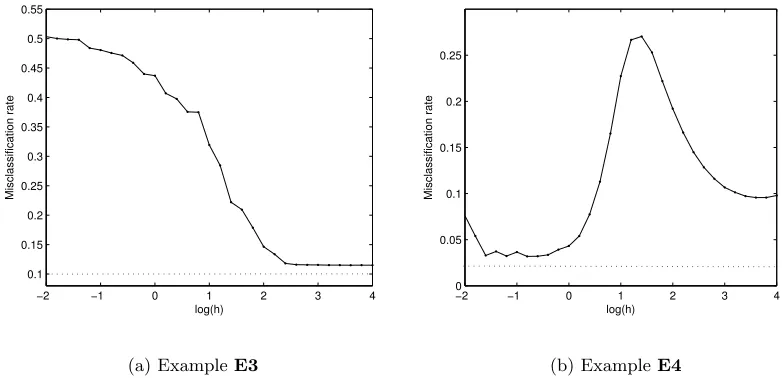
We now consider two examples to demonstrate the above points. The first example (we call it E3) involves two multivariate normal distributions Nd(0d,Id) and Nd(1d,4Id). In the second example (we call it E4), both the competing classes have trimodal distri-butions. The first class has the same density as in Figure 4(a) (i.e., an equal mixture of Nd(0d,0.25Id), Nd(21d,0.25Id) and Nd(41d,0.25Id)), while the second class is an equal mix-ture of Nd(1d,0.25Id), Nd(31d,0.25Id) and Nd(51d,0.25Id). In each of these examples, we consideredd= 5 and generated a training sample of size 100 from each class. The misclassi-fication rate for the classifier based on LSPD◦h was computed based on a test sample of size 500 (250 observations from each class). This procedure was repeated 100 times to calculate the average misclassification rates for different values ofh. Small values ofhextracted local distributional features and yielded low misclassification rates inE4(see Figure 6(b)). How-ever, those small values ofh led to relatively higher misclassification rates inE3, while the underlying global elliptic structure was captured well by the proposed classifier for larger values of h (see Figure 6(a)). This provides a strong motivation for adapting a multi-scale approach in constructing the final classifier so that one can harness the strength of different classifiers corresponding to different scales of localization. One would expect that when aggregated judiciously, the multi-scale classifier will lead to an improved misclassification rate. Usefulness of the multi-scale approach in combining different classifiers has been dis-cussed in the classification literature (see, e.g., Kittler et al., 1998; Dzeroski and Zenko, 2004; Ghosh et al., 2005, 2006).
−2 −1 0 1 2 3 4
0.1 0.15 0.2 0.25 0.3 0.35 0.4 0.45 0.5 0.55
log(h)
Misclassification rate
(a) ExampleE3
−20 −1 0 1 2 3 4
0.05 0.1 0.15 0.2 0.25
log(h)
Misclassification rate
(b) ExampleE4
Figure 6: Misclassification rates of the Bayes classifier (indicated by dotted lines) and the classifier based on LSPD◦h (indicated by solid curves) in examplesE3and E4for varying choices ofh.
A popular way of aggregation is to consider a weighted average of the estimated posterior probabilities computed for different values of h. There are various proposals for the choice of the weight function in the literature. Following Ghosh et al. (2005, 2006), we compute
b
(or, LSPD∗h) and use
W(h)∝exp
"
−1 2
(∆bh−∆b0)2 b
∆0(1−∆0)b /n #
as the weight function, where ∆b0 = minh∆bh. The exponential function helps to
appro-priately weigh up (respectively, weigh down) the promising (respectively, the unsatisfac-tory) classifier resulting from different choices of the smoothing parameter h. We compute
R
W(h)˜g(h)˜p(j|z∗h(x))dhfor thej-th class (1≤j≤J), where a probability density function ˜
g is used to make the integral finite. Here ˜p(j|z∗h(x)) is as defined in equations (4) and (5) of Section 3. If we use very small values ofhto classify a test case, then the kernel function used in LSPDh will put almost zero weights on all observations. Clearly, those small values of h will not be useful for classification. On the other hand, LSPDh behaves like SPD for large values of h. So, after a certain threshold value, increasing the value of h will not provide any additional information about the distributional features. Therefore, one needs to find suitable lower and upper limits ofhto compute the weighted posterior probabilities of different classes. Following Ghosh et al. (2006), we compute the pairwise distances (stan-dardized pairwise distances in the case of LSPD∗h) among the observations in a class and compute the quantiles of these distances. Letλj,α denote theα-th quantile (0< α <1) of the pairwise distances for thej-th class with 1≤j≤J. We usehL= minj{λj,0.05}/3 as the lower limit ofh, andhU = 2rhL as the upper limit of h. Here r is the smallest integer for which we havekz∗h(xji)−z∗(xji)k/kz∗(xji)k<0.05 (or,kz◦h(xji)−z◦(xji)k/kz◦(xji)k<0.05 in case of LSPD◦h) for 1 ≤ i ≤ nj and 1 ≤ j ≤ J. Our final classifier, which we call the LSPD classifier, assigns an observationx to the classj0, where
j0= argmax 1≤j≤J
hU Z
hL
W(h)˜g(h)˜p(j|z∗h(x))dh.
One can choose ˜g to be the uniform distribution on the interval [hL, hU]. Since we are dealing with a scale parameterh, we take the uniform distribution in the logarithmic scale. In practice, we generate M independent observations h1, . . . , hM from the distribution ˜g. For any given 1≤j≤J and x,RhU
hL W(h)˜g(h)˜p(j|z
∗
h(x))dhis approximated by the average
PM
i=1W(hi)˜p(j|z∗hi(x))/M.
5. Analysis of Simulated Data Sets
We have analyzed several data sets simulated from elliptic as well as non-elliptic distribu-tions in R5. In each example, taking an equal number of observations from each of the two
For the classifiers based on SPD and LSPD, we wrote our own R codes and they are available at the link goo.gl/E5tmd6. Throughout this article, we have used 50 different values ofhfor multi-scale classification based on LSPD, and the weight function is computed using 5-fold cross-validation method. In this section and in Section 6, we have used SPD∗ and LSPD∗h for classification with the usual sample covariance matrix of the j-th class as
ˆ
Σj for 1≤j≤J. Any other choice of ˆΣj has been mentioned at appropriate places. We compared our proposed classifiers with a pool of classifiers that include parametric classifiers like LDA and QDA, and nonparametric classifiers like those based onk-NN (with the Euclidean metric as the distance function) and KDE (with the Gaussian kernel). For
k-NN and KDE, we have used the pooled sample covariance matrix for standardization. Tables 1 and 2 show misclassification rates for the multi-scale versions of k-NN (Ghosh et al., 2005) and KDE (Ghosh et al., 2006) based on the same weight function described in Section 4. For the multi-scale method based on KDE, we have considered 50 equi-spaced values of the bandwidth in the range suggested by Ghosh et al. (2006). For the multi-scale version of k-NN, we considered all possible values of k (see Ghosh et al., 2005, for more details). These multi-scale versions usually had better performance then their single scale analogs with the smoothing parameters chosen by the method of cross-validation.
We also considered support vector machines (SVM) (Hastie et al., 2009) based on the linear kernel (i.e., K(x,y) = hx,yi) and the radial basis function (RBF) kernel (i.e.,
Kγ(x,y) = exp(−γkx−yk2)) to facilitate comparison. We used the codes available at theR librarye1071 (Dimitriadou et al., 2011). For the RBF kernel, it has been suggested in the literature to use γ = 1/d (see http://www.csie.ntu.edu.tw/~cjlin/libsvm/). However, for our numerical work, we considered γ = i/10d for 1 ≤i ≤ 50. We also used 25 different values for the box constraint in the interval [0.1,100], which were equi-spaced in the logarithmic scale. Misclassification rates were computed for these different choices of the tuning parameters, and the best result is reported in the tables for both classifiers.
Misclassification rates are also reported for classification tree (TREE), and a boosted version of TREE known as random forest (RF) (see, e.g., Hastie et al., 2009). For the implementation of TREE and RF, we used the R codes available in the libraries tree
(Ripley, 2011) andrandomForest (Liaw and Wiener, 2002), respectively. For classification tree, the deviance function was used as a measure of impurity, and the maximum height of the tree was restricted to 31. Nodes with less than 5 observations were never considered for splitting. We have combined the results of 500 trees in RF, where each tree was generated based on 63.2% randomly chosen observations from the training sample. At any stage, only a random subset of b√dc out of dvariables were considered for splitting. Herebtc denotes the largest integer less than, or equal tot.
(Kosiorowski and Zawadzki, 2016) and considered the best result obtained for different choices of depth and a range of values for the localization parameter. The misclassification rates of the maximum LD classifier was higher than those of the DD classifier in almost all cases, and we do not report those results in this article.
5.1 Examples Involving Elliptic Distributions
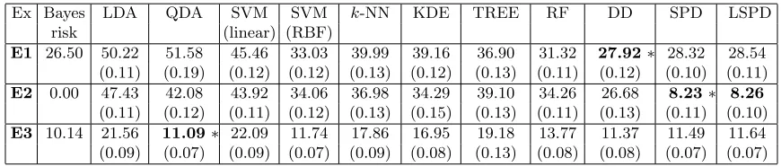
Recall examples E1 and E2 in Section 2, and example E3 in Section 4 involving elliptic class distributions. In E1, the DD classifier led to the lowest misclassification rate closely followed by SPD and LSPD classifiers (see Table 1), but it did not perform well in E2. In this example, SPD and LSPD classifiers significantly outperformed all their competitors. Since the class distributions were elliptic, the SPD classifier had a slight edge over the LSPD classifier in these examples. In view of normality of the class distributions, QDA was expected to have the best performance in E3. The DD classifier ranked second here, while SPD and LSPD classifiers performed satisfactorily. In all these examples, the Bayes classifier had non-linear class boundaries. So, LDA and SVM with the linear kernel did not perform well. The performance of SVM with the RBF kernel was relatively better, and it had competitive misclassification rates inE3. In all these examples, nonparametric classifiers based on k-NN and KDE yielded much higher misclassification rates compared to SPD and LSPD classifiers.
Table 1: Misclassification rates (in %) of different classifiers in elliptic data sets.
Ex Bayes LDA QDA SVM SVM k-NN KDE TREE RF DD SPD LSPD risk (linear) (RBF)
E1 26.50 50.22 51.58 45.46 33.03 39.99 39.16 36.90 31.32 27.92∗ 28.32 28.54 (0.11) (0.19) (0.12) (0.12) (0.13) (0.12) (0.13) (0.11) (0.12) (0.10) (0.11)
E2 0.00 47.43 42.08 43.92 34.06 36.98 34.29 39.10 34.26 26.68 8.23∗ 8.26
(0.11) (0.12) (0.11) (0.12) (0.13) (0.15) (0.13) (0.11) (0.13) (0.11) (0.10)
E3 10.14 21.56 11.09∗ 22.09 11.74 17.86 16.95 19.18 13.77 11.37 11.49 11.64 (0.09) (0.07) (0.09) (0.07) (0.09) (0.08) (0.13) (0.08) (0.08) (0.07) (0.07)
5.2 Examples Involving Non-elliptic Distributions
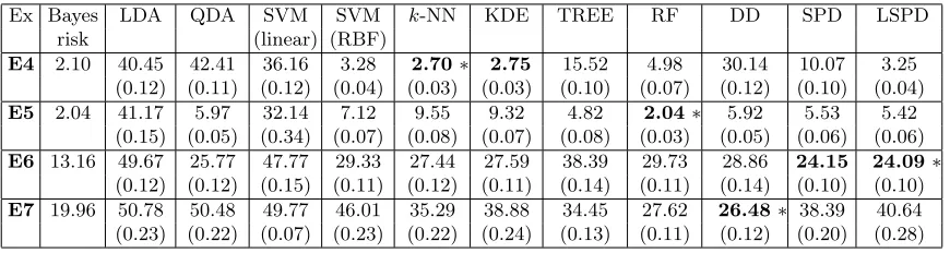
We now consider some examples involving non-elliptic class distributions. Recall the tri-modal example E4 discussed in Section 4. In this example, when the classifiers based on
k-NN and KDE were used after standardizing the data set by the pooled sample covariance matrix, they yielded misclassification rates higher than 40%. For KDE, we used a common bandwidth in all directions after standardization. This lead to the use of a large bandwidth in the principal component direction √1
d1d (this can be observed from Figure 4(a)). Since the difference between the posterior probabilities of the two classes changes its sign fre-quently along this direction, use of this large bandwidth makes it difficult to discriminate between the two competing classes. In thek-NN classifier, this standardization leads to the use of a neighborhood which was also elongated along the direction √1
standard-ization. So we used classifiers based on SPD◦ and LSPD◦ in this example. The LSPD◦ classifier had the third best performance. SVM with the RBF kernel also performed well. All other classifiers had relatively higher misclassification rates. The DD classifier, LDA, QDA and SVM with the linear kernel all misclassified more than 25% of the observations.
The next example (we call it E5) is with exponential distributions, where the com-ponent variables are independently distributed in both classes. The i-th variable in the first (respectively, the second) class is exponential with scale parameter d/(d−i+ 1) (re-spectively, d/2i) for 1 ≤ i ≤ d. Further, the second class has a location shift such that the difference between the mean vectors of the two classes is 1d1d. Recall that Figure 5(a) shows the density contours of the first class when d = 2. In this example, the RF classi-fier had the best performance followed by TREE. Here all the measurement variables were independent, and there was significant separation between the two classes in some of the co-ordinate directions. This is one of the main reasons behind the superior performance of both TREE and RF. Classifiers based on DD, SPD∗ and LSPD∗ also performed quite well, and their misclassification rates were significantly lower than all other classifiers. The two linear classifiers performed poorly, but QDA had a reasonably good performance in this example. Good performance of QDA was not surprising as the two competing classes are unimodal, while they differ widely in their dispersion structures.
Table 2: Misclassification rates (in %) of different classifiers in non-elliptic data sets.
Ex Bayes LDA QDA SVM SVM k-NN KDE TREE RF DD SPD LSPD risk (linear) (RBF)
E4 2.10 40.45 42.41 36.16 3.28 2.70∗ 2.75 15.52 4.98 30.14 10.07 3.25 (0.12) (0.11) (0.12) (0.04) (0.03) (0.03) (0.10) (0.07) (0.12) (0.10) (0.04)
E5 2.04 41.17 5.97 32.14 7.12 9.55 9.32 4.82 2.04∗ 5.92 5.53 5.42 (0.15) (0.05) (0.34) (0.07) (0.08) (0.07) (0.08) (0.03) (0.05) (0.06) (0.06)
E6 13.16 49.67 25.77 47.77 29.33 27.44 27.59 38.39 29.73 28.86 24.15 24.09∗
(0.12) (0.12) (0.15) (0.11) (0.12) (0.11) (0.14) (0.11) (0.14) (0.10) (0.10)
E7 19.96 50.78 50.48 49.77 46.01 35.29 38.88 34.45 27.62 26.48∗ 38.39 40.64 (0.23) (0.22) (0.07) (0.23) (0.22) (0.24) (0.13) (0.11) (0.12) (0.20) (0.28)
In example E6, each class is an equal mixture of four elliptic distributions. The first class constitutes of Nd(1d, S0.6), t3,d(βd, S0.7), Nd(−1d, S0.8) and t3,d(−βd, S0.9), while the second class is an equal mixture of t3,d(1d, S−0.9), Nd(βd,3S−0.8), t3,d(−1d, S−0.7) and
Nd(−βd,3S−0.6). Heret3,d(µ,Σ) denotes the d-variatetdistribution with 3 degrees of free-dom (df), location parameterµand scatter matrixΣ. The vectorβdis ad-dimensional vec-tor with thei-th element equal to (−1)i+1 for 1≤i≤dand the matrixS
α = ((α|i−j|))d×d for α ∈ (−1,1) and 1 ≤ i, j ≤ J. This example has a complex structure for the class distributions, and both SPD and LSPD classifiers significantly outperformed all their com-petitors. As the Bayes classifier was far from being linear, LDA and linear SVM did not have satisfactory performance.
relatively higher misclassification rates. Both half-space depth and projection depth used in the DD classifier are robust against outliers generated from heavy-tailed distributions, while the moment based estimates used in both SPD∗ and LSPD∗ are non-robust. So, it is better to use robust estimates ofΣjs here. When we used MCD estimates based on 75% of the observations (Rousseeuw and Van Driessen, 1999), the misclassification rates of SPD∗ and LSPD∗ classifiers dropped to 31.90% and 32.05%, respectively, with corresponding standard errors of 0.18% and 0.20%.
All these examples clearly demonstrate that the LSPD classifier performs as good as (if not better) popular nonparametric classifiers for non-elliptic, or multi-modal data. This adjustment of the LSPD classifier is automatic in view of the multi-scale approach developed in Section 4.
5.3 Computing Time for SPD and LSPD Classifiers
For a training sample of sizen, computation ofz(xji) for 1≤i≤nj and 1≤j≤J requires
O(n2) calculations. Fitting a GAM involves an iterative algorithm, and it is quite difficult to calculate its exact computational complexity. Each iteration requires computations of the orderO(n2) (Wood, 2006). So, the algorithm takes no more than O(n2) computations to fit a GAM for a finite number of iterations. For the multi-scale classifier based on LSPD, we need to repeat this procedure for M different values ofh and then compute the weight functionW(h) based on V-fold cross-validation. The overall order of computation remains
O(n2) although the associated constant increases linearly with d, J,M and V. However, one should note that these are offline calculations. Both SPD and LSPD classifiers require
O(n) calculations to classify a test case.
Throughout this article, we have used M = 50 andV = 5 and theRlibrary VGAM (Yee, 2008) was used to fit GAM. In a single iteration, the average CPU time to determine the weight functionW(h) based on cross-validation for the LSPD classifier was 21.83 seconds, while 0.55 seconds were required to fit a GAM using the full training data. The average CPU time to classify the 500 test observations was about 0.01 seconds. All the calculations were done on a desktop computer with an Intel i7 (2.2 GHz) processor having 8 GB RAM.
6. Analysis of Benchmark Data Sets
We have analyzed seven benchmark data sets for further evaluation of our proposed classi-fiers. The biomedical data set is taken from the CMU data archive (http://lib.stat.
cmu.edu/datasets/). In this data set, we ignored the observations with missing
val-ues. The diabetes data set is available in the R library mclust (also analyzed in Reaven and Miller, 1979). All other data are taken from the UCI machine learning repository
(http://archive.ics.uci.edu/ml/). Descriptions of these data sets are available at these
sources. Satellite image (satimage) data set has specific training and test samples. For this data set, we report misclassification rates of different classifiers based on this fixed test set. If a classifier had misclassification rate ε, its standard error was computed as
p
stan-dard errors. Sizes of training and test sets in each partition are also reported in this table. For all classifiers, we used the same tuning procedures as described in Section 5. Codes for the DD classifier are available only for two class problems. In biomedical and Parkinson’s data sets, the DD classifier yielded misclassification rates of 12.54% and 14.48%, respec-tively, with corresponding standard errors of 0.18% and 0.15%. We also used the maximum LD classifier on these real data sets. However, its performance was not satisfactory for most data sets and we do not report those misclassification rates in Table 3.
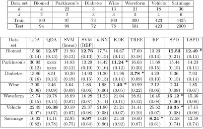
In biomedical and vehicle data, covariance matrices of the competing classes were differ-ent. So, QDA led to significant improvement over LDA, and its misclassification rates were close to the best rate. In both these data sets, the competing classes were nearly elliptic (this can be verified using the diagnostic plots suggested by Li et al., 1997). The SPD classifier utilized this ellipticity of the class distributions to outperform the nonparametric classifiers. The LSPD classifier competed well with the SPD classifier in biomedical data. But, the evidence of ellipticity was much stronger in vehicle data and LSPD had a slightly higher misclassification rate. In diabetes data also, the three competing classes had widely varying covariance structures. As expected, QDA performed better than LDA. Since the class distributions were not elliptic, the SPD classifier yielded a higher misclassification rate than the LSPD classifier, while both TREE and RF outperformed all other classifiers in this data set.
Table 3: Descriptions of the real data sets, and misclassification rates (in %) of different classifiers.
Data set Biomed Parkinson’s Diabetes Wine Waveform Vehicle Satimage
d 4 22 3 13 21 18 36
J 2 2 3 3 3 4 6
Train 100 97 73 100 300 423 4435
Test 94 98 72 78 501 423 2000
Data LDA QDA SVM SVM k-NN KDE TREE RF SPD LSPD set (linear) (RBF)
Biomed 15.66 12.57 21.90 12.76 17.74 16.67 17.69 13.23 12.53 12.49 *
(0.14) (0.13) (0.13) (0.13) (0.15) (0.14) (0.18) (0.14) (0.21) (0.15) Parkinson’s 30.93 xxxx 14.83 13.29 14.42 11.24 * 16.63 11.68 15.44 14.23 (0.12) xxxx (0.12) (0.10) (0.16) (0.12) (0.20) (0.15) (0.15) (0.11) Diabetes 13.86 8.51 10.20 14.93 11.20 11.96 3.78 * 4.29 9.36 7.93
(0.16) (0.13) (0.19) (0.15) (0.13) (0.14) (0.09) (0.10) (0.15) (0.14)
Wine 2.00 2.46 3.64 1.86 1.98 1.40 * 10.99 2.12 2.34 1.85
(0.06) (0.09) (0.09) (0.06) (0.06) (0.05) (0.22) (0.06) (0.08) (0.07) Waveform 19.74 20.78 18.89 16.28 21.23 21.04 28.81 16.45 15.12 * 15.36 (0.15) (0.15) (0.07) (0.07) (0.11) (0.11) (0.12) (0.08) (0.06) (0.06) Vehicle 22.49 16.38 20.59 25.37 21.80 21.21 31.41 25.52 16.35 * 17.15 (0.07) (0.07) (0.07) (0.08) (0.08) (0.07) (0.10) (0.07) (0.08) (0.08) Satimage 16.02 14.11 12.95 8.97 18.00 21.40 18.60 8.24 * 12.58 12.58 (0.82) (0.78) (0.75) (0.64) (0.86) (0.92) (0.87) (0.61) (0.74) (0.74)
‘xxxx’: QDA could not be used because of singularity of the estimated class dispersion matrices.
of SPD∗ and LSPD∗. In this data set, all the nonparametric classifiers had significantly lower misclassification rates than LDA, and the classifier based on KDE had the lowest misclassification rate. The performance of the LSPD classifier was also competitive. Since the underlying distributions were non-elliptic, LSPD outperformed the SPD classifier. We observed a similar phenomena in wine data as well. The sample covariance matrices of different classes were nearly singular, and we used the pooled sample covariance matrix for computing SPD∗ and LSPD∗. The classifier based on KDE yielded the lowest misclassi-fication rate, while the LSPD classifier had the second best performance. Although the data dimension was quite high in both data sets, all the competing classes had low intrinsic dimensions (can be estimated using the method described by Levina and Bickel, 2004). So, nonparametric methods like KDE were not affected much by the curse of dimensionality. TREE was the only classifier with a somewhat higher misclassification rate.
In waveform data, the competing class distributions were nearly elliptic and the SPD classifier was expected to perform well. The LSPD classifier is quite flexible, and it yielded a competitive misclassification rate. The class distributions were not normal (can be checked using the method proposed in Royston, 1983) for this data, and did not have low intrinsic dimensions. As a result, LDA, QDA and the nonparametric classifiers had relatively higher misclassification rates.
In satimage data, recall that the results are based on a single training and a single test set. So, the standard errors of the misclassification rates were high for all classifiers, and it is quite difficult to compare the performance of different classifiers. Both RF and SVM with the RBF kernel had lower misclassification rates than other classifiers, while the classifiers based on SPD and LSPD had the next best performance.
7. Classification of High-dimensional Data
A serious practical limitation of many existing depth based classifiers is their computational complexity in high dimensions, and this makes such classifiers impossible to use even for moderately large dimensional data. Besides, depth functions that are based on random simplices formed by the data points (see, e.g., Liu et al., 1999; Zuo and Serfling, 2000) cannot be defined in a meaningful way if the dimension of the data exceeds the sample size. Tukey’s half-space depth and projection depth both become degenerate at zero for such high-dimensional data (see, e.g., Dutta et al., 2011). Classification of high-dimensional data presents a substantial challenge to many nonparametric classification tools as well. We have seen in examples E1 and E2 (recall Figure 2) that nonparametric classifiers like those based on k-NN and KDE can yield poor performance when the data dimension is large. Some limitations of SVM for classification of high-dimensional data has been noted by Marron et al. (2007); Dutta and Ghosh (2016).
(C) Consider two independent random vectors X1 = (X1(1), . . . , X (d)
1 )T ∼ Fj and X2 = (X2(1), . . . , X2(d))T ∼F
i for 1≤j, i≤J. Further, assume that
(C1)aj = limd→∞d−1 Pkd=1E(X1(k))2 exists, andd−1Pdk=1(X1(k))2 a.s.→ aj asd→ ∞, (C2)bji= limd→∞d−1Pdk=1E(X1(k)X2(k)) exists, andd−1Pdk=1X1(k)X2(k)a.s.→ bji asd→ ∞.
It is not difficult to verify that forX1 ∼Fj (1≤j≤J), if we assume that the sequence of variables {X1(k)−E(X1(k)) :k = 1,2, . . .} centered at their means are independent with uniformly bounded eighth moments (see Theorem 1 (2) in Jung and Marron, 2009, p. 4110), or they are m-dependent processes with some appropriate conditions (see Theorem 2 in de Jong, 1995, p. 350), then the convergence results in (C1) and (C2) hold. Also, if the observations are generated from discrete time ARMA processes, all these conditions are satisfied. Stationarity of such time series is not required here. These assumptions continue to hold if the sequences{(X1(k))2−E(X1(k))2 :k= 1,2, . . .}and{X1(k)X2(k)−E(X1(k)X2(k)) :
k = 1,2, . . .}, where X1 ∼ Fj and X2 ∼ Fi for all 1 ≤ j, i ≤ J, are mixingales satisfying some appropriate conditions (see, e.g., Theorem 2 in de Jong, 1995, p. 350).
Define σ2j =aj−bjj andνji =bjj−2bji+bii. For the random vector X1∼Fj,σ2j is the limit ofd−1Pd
k=1V ar(X (k)
1 ) asd→ ∞. If we consider a second independent random vector
X2 ∼ Fi with i 6= j, then νji is the limit of d−1Pdk=1{E(X1(k))−E(X2(k))}2 as d → ∞. Hall et al. (2005) assumed a similar set of conditions to study the performance of support vector machines (SVM) with the linear kernel and the 1-NN classifier as the data dimension grows to infinity. Similar conditions on observation vectors were also considered by Jung and Marron (2009) to study consistency of principal components of the empirical covariance matrix for high-dimensional data. Under (C1) and (C2), the following theorem describes the behavior ofz◦(x) = (SPD◦(x, F1),. . ., SPD◦(x, FJ))T and z◦h(x) = (LSPD
◦
h(x, F1),. . ., LSPD◦h(x, FJ))T asdgrows to infinity.
Theorem 6 Suppose that the conditions (C1)-(C2) hold, and X∼Fj for 1≤j ≤J. (a) z◦(X)a.s.→ (cj1, . . . , cjJ)T =cj asd→ ∞, wherecjj = 1−
q
1
2 andcji = 1−
r
σ2
j+νji
σ2
j+σ2i+νji for 1≤j6=i≤J.
(b) Assume that h → ∞ and d → ∞ in such a way that √d/h → 0 or A0(> 0). Then, z◦h(X)a.s.→ g0(0)cj or c0j = (g0(ej1A0)cj1, . . . , g0(ejJA0)cjJ)T depending on whether
√
d/h→
0or A0, respectively. Here K(t) =g0(ktk),ejj = √
2σj andeji =
q
σ2j +σ2i +νjifor j6=i. (c) Assume thath >1, and√d/h→ ∞ as d→ ∞. Then, z◦h(X)a.s.→ 0J.
at a rate faster thanh,z◦h(x) converges to the same value0J and it becomes non-informative. Consequently, the classifier based on LSPD◦h will lead to a high misclassification probability in this case.
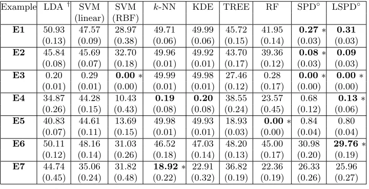
To evaluate the performance of our depth based classifiers for high-dimensional data, we considered examples E1-E7 with d= 200. In each example, we generated 20 observations from each class to constitute the training sample, while 250 observations from each class were used to form the test set. We generated 500 training and test sets, and the average test set misclassification rates of the different classifiers along with their corresponding standard errors are reported in Table 4. The Bayes risks werealmost zeroin all these examples, and we have not stated them in Table 4. We did not standardize the data for KDE andk-NN. QDA could not be used in these examples, and we used Id instead of the pooled sample covariance matrix for LDA. When the competing classes have equal priors (which is the case in simulated examples), this leads to the Euclidean distance based classifier which classifies an observation to the class having the nearest centroid.
As we have mentioned before, we use SPD◦ and LSPD◦ for classification of these high-dimensional data sets. For a single iteration, the LSPD classifier required an average CPU time of 8.82 seconds to compute the weight function W(h), 0.39 seconds for fitting GAM using the full training data, and 0.06 seconds for classification of 500 test cases.
Table 4: Misclassification rates (in %) of different classifiers in simulated data sets.
Example LDA† SVM SVM k-NN KDE TREE RF SPD◦ LSPD◦ (linear) (RBF)
E1 50.93 47.57 28.97 49.71 49.99 45.72 41.95 0.27∗ 0.31
(0.13) (0.09) (0.38) (0.06) (0.06) (0.15) (0.14) (0.03) (0.03)
E2 45.84 45.69 32.70 49.96 49.92 43.70 39.36 0.08∗ 0.09
(0.08) (0.07) (0.18) (0.01) (0.01) (0.17) (0.12) (0.03) (0.03)
E3 0.20 0.29 0.00∗ 49.99 49.98 27.46 0.28 0.00∗ 0.00∗
(0.01) (0.01) (0.00) (0.01) (0.01) (0.12) (0.17) (0.00) (0.00)
E4 34.87 44.28 10.43 0.19 0.20 38.55 23.57 0.68 0.13∗
(0.26) (0.15) (0.43) (0.08) (0.08) (0.24) (0.45) (0.12) (0.06)
E5 40.83 44.61 13.69 49.98 49.93 18.93 0.00∗ 0.84 0.80 (0.07) (0.11) (0.15) (0.01) (0.01) (0.03) (0.00) (0.04) (0.04)
E6 50.11 48.16 31.03 46.52 47.03 48.20 45.00 30.98 29.76∗
(0.12) (0.14) (0.26) (0.18) (0.14) (0.13) (0.17) (0.20) (0.19)
E7 44.74 35.06 31.82 18.92∗ 22.91 36.82 22.36 26.33 25.96 (0.45) (0.24) (0.48) (0.22) (0.32) (0.19) (0.19) (0.26) (0.27)
†
Idwas used instead of the pooled sample covariance matrix.
distribution from the first class and one from the second class differ only in their scales, the k-NN classifier gives a decision in favor of the distribution with a smaller spread (also see Hall et al., 2005). This was the main reason behind the poor performance of the k-NN classifier. Similar arguments can be given for the poor performance of the classifier based on KDE. In these two examples, splitting based on a single variable failed to yield significant reduction in the impurity function (one can see this in Figure 1). So, TREE and RF had relatively higher misclassification rates. In E3, the two Gaussian distributions differed in their locations and scales. Barring TREE,k-NN and the classifier based on KDE, all other classifiers yielded misclassification rates close to zero. Since the scale difference between the two classes dominates the location difference, such a poor performance of the classifier based on KDE and k-NN was expected (see the results in Hall et al., 2005; Dutta and Ghosh, 2016). The same explanation holds for E5as well. These nonparametric classifiers yielded excellent performance inE4, where the component distribution differ only in their locations. However, TREE and RF failed to have satisfactory performance here. Splitting based on linear combinations of the variables may be helpful inE4(see Figure 4).
Examples E6and E7 were difficult to deal with. Unlike E1-E5, none of the classifiers could achieve misclassification rates close to zero in these two examples. Conditions (C1) and (C2) do not hold here, and Theorem 6 is not applicable. The LSPD classifier had the best performance in E6 (just like the case with d = 5 in Section 5). SVM with the RBF kernel and the SPD classifier also led to competitive misclassification rates. Their performance was much better than all other classifiers. In E7, the linear classifiers and SVM with the RBF kernel could not perform well. This is also consistent with what we observed in Section 5. Barring TREE, all other classifiers yielded competitive performances in this example. Among them thek-NN classifier led to the lowest misclassification rate.
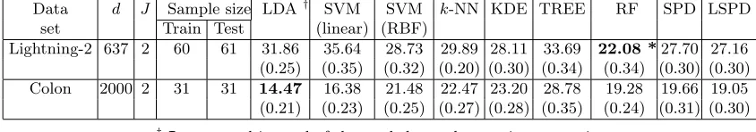
We also analyzed two high-dimensional benchmark data sets, namely, lightning-2 data and colon data (Alon et al., 1999). The first data set is from the UCR time series classi-fication archive (http://www.cs.ucr.edu/~eamonn/time_series_data/), while the other one is taken from the R library rda. In each case, we formed 500 training and test sets by randomly partitioning each data into two almost equal parts. The average test set misclassification rates of different classifiers are reported in Table 5.
Table 5: Misclassification rates (in %) of different classifiers in real data sets.
Data d J Sample size LDA† SVM SVM k-NN KDE TREE RF SPD LSPD set Train Test (linear) (RBF)
Lightning-2 637 2 60 61 31.86 35.64 28.73 29.89 28.11 33.69 22.08 *27.70 27.16 (0.25) (0.35) (0.32) (0.20) (0.30) (0.34) (0.34) (0.30) (0.30) Colon 2000 2 31 31 14.47 16.38 21.48 22.47 23.20 28.78 19.28 19.66 19.05 (0.21) (0.23) (0.25) (0.27) (0.28) (0.35) (0.24) (0.31) (0.30)
†
Idwas used instead of the pooled sample covariance matrix.
Colon data contain micro-array expression levels of 2000 genes for ‘normal’ and ‘colon cancer’ tissues. There was a good linear separation among the observations from the two competing classes, and the linear classifiers lead to low misclassification rates. Among the other classifiers, the LSPD classifier yielded the minimum misclassification rate closely followed by RF and the SPD classifier. These three classifiers were less affected by the curse of dimensionality.
In these high-dimensional benchmark data sets, the data had low intrinsic dimensions due to high correlation among the the measurement variables (Levina and Bickel, 2004). Moreover, data from the competing classes differed mainly in their locations. As a conse-quence, though the proposed LSPD classifier had a good overall performance, its superiority over the nonparametric methods was not as prominent as it was in the simulated examples.
Acknowledgments
The authors are grateful to Prof. Probal Chaudhuri for his valuable contributions to this manuscript. They are also thankful to the Action Editor and two anonymous reviewers for providing them with several helpful comments. The first author would like to thank Prof. Thomas W. Yee for his help with VGAM, and Prof. Jun Li for sharing R codes of the DD classifier.
Appendix A. Proofs and Mathematical Details
Lemma 7 If F has a spherically symmetric densityf(x) =g(kxk) onRd withd >1, then
kEF[u(x−X)]k is a non-negative monotonically increasing function ofkxk.
Proof of Lemma 7 : In view of spherical symmetry of f(x), S(x) =kEF[u(x−X)]k is invariant under orthogonal transformations of x. Consequently, S(x) = η(kxk) for some non-negative function η. Consider now x1 and x2 such that kx1k<kx2k. Using spherical symmetry off(x), without loss of generality, we can assumexi = (ti,0, . . . ,0)T fori= 1,2 such that|t1|<|t2|. For anyx= (t,0, . . . ,0)T, we have
S(x) =
EF
(t−X1)
q
(t−X1)2+X2
2 +. . .+Xd2
,
due to spherical symmetry of f(x). For anyx∈ Rd withd >1, EF[kx−Xk] is a strictly convex function ofxin this case. Consequently, it is a strictly convex function oft. Observe now that S(x) with this choice ofx is the absolute value of the derivative of EF[kx−Xk] w.r.t. t. This derivative is a symmetric function of tthat vanishes att= 0. Hence,S(x) is an increasing function of|t|, and this proves that η(kx1k)< η(kx2k).
Proof of Theorem 1 : If the population distribution fj(x) is elliptically symmetric, we have fj(x) = |Σj|−1/2gj(δ(x, Fj)), where δ(x, Fj) = kΣ
−1/2
j (x−µj)k is the Mahalanobis distance for 1≤j≤J. Since SPD∗(x, Fj) = 1−kE[u(Σ
−1/2
with its center at the origin, from Lemma 7 it follows that SPD∗(x, Fj) is a monotonically decreasing function of δ(x, Fj). Therefore, δ(x, Fj) is also a function of SPD∗(x, Fj) and using this factfj(x) can also be expressed as
fj(x) =ψj(SPD∗(x, Fj)) for all 1≤j≤J,
where ψj is an appropriate real-valued function that depends on gj. Now, one can check that
log
hp(j|x)
p(J|x)
i
= log(πj/πJ) + logψj(SPD∗(x, Fj))−logψJ(SPD∗(x, FJ)).
for 1 ≤ j ≤ (J −1). Now, if we define ϕjj(z) = logπj + logψj(z) and ϕij(z) = 0 for 1≤j6=i≤(J−1); and ϕ1J(z) =· · ·=ϕ(J−1)J(z) =−logπJ −logψJ(z), then the proof is complete.
Remark 8 If fj(x) is unimodal, ψj(z) is monotonically increasing for 1≤ j ≤J.
More-over, if the distributions differ only in their locations, then theψjs are same for all classes.
In that case, fj(x) > fi(x) ⇔ δ(x, Fj) < δ(x, Fi) ⇔ SPD∗(x, Fj) > SPD∗(x, Fi) for 1≤i6=j ≤J, and hence the classifier turns out to be the maximum SPD classifier.
Proof of Theorem 3(a) : Let h <1. For any fixed x∈Rd and the distribution function
Fj, we have LSPD∗h(x, Fj) =EFj[Kh(t)]− kEFj[Kh(t)u(t)]k,wheret=Σj
−1/2(x−X) for 1≤j≤J. For the first term in the expression of LSPD∗h(x, Fj) above, we have
EFj[Kh(t)] = Z
Rd
1
hdKh(Σ
−1/2
j (x−v))fj(v)dv=|Σj| 1/2
Z
Rd
K(y)fj(x−hΣ1j/2y)dy,
wherey=h−1Σ−1/2
j (x−v). So, using Taylor’s expansion offj(x), we get
EFj[Kh(t)] =|Σj|
1/2f
j(x)−h|Σj|1/2
Z
Rd
K(y) (Σ1j/2y)T∇fj(ξ)dy,
whereξ lies on the line joiningxand (x−hΣ1j/2v). Using the Cauchy-Schwartz inequality, one gets
EFj[Kh(t)]−|Σj|
1/2f j(x)
≤h|Σj|
1/2λ1/2
j Mj◦MK, whereMj◦= supx∈Rdk∇fj(x)k,
MK =
R
kykK(y)dy, and λj is the largest eigenvalue of Σj. This implies
EFj[Kh(t)]−
|Σj|1/2fj(x)
→0 as h→0 for 1≤j≤J.
For the second term in the expression of LSPD∗h(x, Fj), a similar argument yields
EFj[Kh(t)u(t)] =|Σj|
1/2Z
Rd
K(y)u(y)fj(x−hΣ1j/2y)dy =−h|Σj|1/2
Z
Rd
K(y)u(y) (Σj1/2y)T∇fj(ξ)dy (as
Z
Rd
K(y)u(y)dy=0).
Now, kEFj[Kh(t)u(t)]k ≤ h|Σj|
1/2λ1/2 j M
◦
Proof of Theorem 3(b) : Here we consider the case h > 1. Take any fixed x ∈ Rd and a j with 1 ≤ j ≤ J. For any fixed t, since K(t/h) → K(0) as h → ∞ and K is bounded, using Dominated Convergence Theorem (DCT), one can show that LSPD∗h(x, Fj) → K(0)SPD∗(x, Fj) as h → ∞. So, z∗h(x) → (K(0)SPD∗(x, F1), . . . , K(0) SPD∗(x, FJ))T ash→ ∞.
Proof of Theorem 5 : Define the sets Bn = {x = (x1, . . . , xd) : kxk ≤ √
dn}, and
An ={x: n2xi is an integer and |xi| ≤n for all 1 ≤i≤d}. Clearly An ⊂Bn ⊂ Rd, the
setBnis a closed ball and the setAnhas cardinality (2n3+ 1)d. We will prove almost sure (a.s.) uniform convergence on three disjoint sets: (i) An, (ii) Bn\An and (iii) Bnc.
Consider any fixed h ∈(0,1]. Recall that for this choice of h, LSPD◦h(x, F) (see equation (3)) and LSPD◦h(x, Fn) are defined as follows:
LSPD◦h(x, Fn) = 1
nhd n
X
i=1
Kx−Xi h − 1 nhd n X i=1
Kx−Xi h
u(x−Xi)
, and
LSPD◦h(x, F) = 1
hdE
h
Kx−X h i − 1 hd E h
Kx−X h
u(x−X)i
.
(i) Define Zi = K(h−1(x−Xi))u(x−Xi)−E[K(h−1(x−X))u(x−X)] for 1 ≤ i ≤ n. Note that Zis are independent and identically distributed (i.i.d.) with E(Zi) = 0 and kZik ≤2K(0). Fix an > 0. Using the exponential inequality for sums of i.i.d. random vectors (see Yurinskii, 1976, p. 491), we obtain P
kn−1Pn
i=1Zik ≥
≤ 2e−C0n2. Here
C0 is a positive constant that depends onK(0) and . This now implies that
P 1 nhd n X i=1 K
x−Xi
h
u(x−Xi)
− 1
hdE
h K
x−X
h
u(x−X)
i ≥ ≤P 1 nhd n X i=1
Kx−Xi h
u(x−Xi)− 1
hdE
h
Kx−X h
u(x−X)i
≥ =P 1 n n X i=1 Zi ≥h
d≤2e−C0nh2d2. (6)
For a fixed value of h,Pn
i=1K(h−1(x−Xi)) is a sum of i.i.d. bounded random variables. Using Bernstein’s inequality, we obtain
P 1 n n X i=1 K
x−Xi
h
−E h
K
x−X
h i
≥
≤2e−C1n2,
for some suitable positive constant C1. This implies
P 1 nhd n X i=1
Kx−Xi h
− 1
hdE
h
Kx−X h
i
≥
≤2e−C1nh2d2. (7)
Combining (6) and (7), we get P(|LSPD◦(x, Fn)−LSPD◦(x, F)| ≥ ) ≤C3e−C4nh
2d2
for some suitable constantsC3 and C4. Since the cardinality of An is (2n3+ 1)d, we have
P
sup
x∈An
|LSPD◦(x, Fn)−LSPD◦(x, F)| ≥
Now, P
n≥1(2n3+ 1)de−C4nh
2d2
<∞. So, an application of Borel-Cantelli lemma implies
that supx∈An|LSPD
◦
h(x, Fn)−LSPD◦h(x, F)| a.s.
→ 0 asn→ ∞.
(ii) Consider the set Bn\An. Given any x in Bn\An, there exists y ∈ An such that kx−yk ≤√2/n2. First we will show that|LSPD◦(y, Fn)−LSPD◦(x, Fn)|
a.s.
→ 0 asn→ ∞. Using the mean-value theorem, one obtains
1 nhd n X i=1
Kx−Xi h − 1 nhd n X i=1
Ky−Xi h ≤ 1
nhd+1 n X i=1
(x−y)T∇Kξ−Xi h
,
whereξlies on the line joiningxandy. Note that the right hand side is less than M
0
K
hd+1 √
2
n2, and MK0 = suptk∇K(t)k. This upper bound is free ofx, and goes to 0 as n→ ∞. Now,
1 nhd n X i=1 K
x−Xi
h
u(x−Xi)
− 1 nhd n X i=1 K
y−Xi
h
u(y−Xi)
≤ 1 nhd n X i=1 h K
x−Xi
h
u(x−Xi)−K
y−Xi
h
u(y−Xi)
i (9) ≤ 1 nhd n X i=1 h K
x−Xi
h
−K
y−Xi
h i
+K(0)
1 nhd n X i=1
[u(x−Xi)−u(y−Xi)]
.
We have proved above that the first part converges to 0 in a.s. sense.
For the second part, consider a ball of radius 1/n aroundx(say, B(x,1/n)). Now,
1 nhd n X i=1
[u(x−Xi)−u(y−Xi)]
≤ 2 nhd n X i=1
I[Xi∈B(x,1/n)]
+2n
hdkx−yk
≤ 2 hd 1 n n X i=1
I[Xi ∈B(x,1/n)]−P[X1 ∈B(x,1/n)]
+ 2
hdP[X1 ∈B(x,1/n)] + 2n√2
n2hd.
Note that I[Xi ∈ B(x,1/n)]s are i.i.d. bounded random variables with expectation
P[X ∈ B(x,1/n)]. Therefore, a.s. convergence of the first term follows from Bernstein’s inequality. Since P[X ∈ B(x,1/n)] ≤ Mfn−d (where Mf = supxf(x) < ∞), the second
term converges to 0. For any fixed h, the third term also converges to 0 as n→ ∞. So, we have |LSPD◦h(x, Fn)−LSPD◦h(y, Fn)|
a.s.
→ 0 as n→ ∞.
Similarly, one can prove that |LSPD◦h(x, F) −LSPDh◦(y, F)| a.s.→ 0 as n → ∞. In the arguments above, all the bounds are free from x and y. We have also proved that supy∈An|LSPD
◦
h(y, Fn)−LSPD◦h(y, F)| a.s.
→ 0 as n→ ∞. Combining all these results, we have supx∈Bn\An|LSPD
◦
h(x, Fn)−LSPD◦h(x, F)| a.s.
→ 0 asn→ ∞.
(iii) Now, consider the region outsideBn (i.e., the setBnc). First note that
sup
x∈Bc n
|LSPD◦h(x, Fn)−LSPD◦h(x, F)| ≤ sup
x∈Bc n 1 nhd n X i=1 K
x−Xi
h
+ sup
x∈Bc n
1
hdE
h K
x−X
h i
We will show that both of these terms become sufficiently small asn→ ∞.
Fix an > 0. We can choose two constants M1 and M2 such that P(kXk ≥ M1) ≤
hd/2K(0) andK(t)≤hd/2 whenktk ≥M2. Now, one can check that 1
hdE
h
Kx−X h
i
≤ 1
hdE
h
Kx−X h
I(kXk ≤M1)
i
+ 1
hdK(0)P(kXk> M1). If x∈Bnc and kXk ≤M1, then h−1kx−Xk ≥h−1|√dn−M1|. Choose nlarge enough so that|√dn−M1| ≥M2h, and this impliesK(h−1(x−X))≤hd/2. So, we obtain
1
hdE
h
Kx−X h
i
≤ 2 +
1
hdK(0)P(kXk> M1)≤, and 1
nhd n
X
i=1
Kx−Xi h
≤ 2+
1
hdK(0) 1
n
n
X
i=1
I(kXik> M1)
≤+ 1
hdK(0)
1 n n X i=1
I(kXik> M1)−P(kXk> M1)
.
The Glivenko-Cantelli theorem implies that the last term on the right hand side converges to 0 as n→ ∞. So, we have supx∈Bc
n|LSPD
◦
h(x, Fn)−LSPD◦h(x, F)| a.s.
→ 0 asn→ ∞.
Combining the arguments in parts (i), (ii) and (iii) and for a fixed h ∈ (0,1], we get supx|LSPD◦h(x, Fn)−LSPD◦h(x, F)|
a.s.
→ 0 asn→ ∞. If we haveh >1, then this convergence result can be proved in a similar way. For this case, recall that the definition of LSPD◦(x, F) does not involve thehdterm in the denominator (see equation (3)).
Remark 9 Following the proof of Theorem 5, it is easy to check that a.s. convergence holds when h diverges to infinity with n.
Remark 10 The result continues to hold when h →0 as well. However, for a.s. conver-gence in part (i) (to use the Borel-Cantelli lemma) we require nh2d/logn→ ∞ asn→ ∞. In part (iii), we need M1 and M2 to vary with n. Assume the first moment of the density
corresponding to F to be finite, and R
ktkK(t)dt < ∞ (which implies that ktkK(t) → 0
as ktk → ∞). Also, assume that nh2d/logn → ∞ as n → ∞. We can now choose M1 = M2 =
√
n to ensure that both P(kXk ≥ M1) ≤ hd/2K(0) and K(t) ≤ hd/2 for ktk ≥M2 hold for a sufficiently large n.
Proof of Theorem 6(a) : Consider two independent random vectors X = (X(1), . . .,
X(d))T ∼Fj and X1 = (X1(1), . . . , X1(d))T ∼Fj, where 1≤j≤J. It follows from (C1) and (C2) thatkX−X1k/
√
da.s.→ q2σ2
j asd→ ∞.So, for almost every realizationxofX∼Fj, kx−X1k/
√
da.s.→
q
2σ2
i asd→ ∞. (10)
Next, consider two independent random vectors X ∼Fj and X1 ∼Fi for 1 ≤i 6=j ≤ J. Using (C1) and (C2), we get kX−X1k/
√
da.s.→ qσj2+σi2+νji as d→ ∞. Consequently, for almost every realizationx ofX∼Fj
kx−X1k/ √
Let us next consider hx−X1,x−X2i, where X ∼ Fj, X1,X2 ∼ Fi are independent random vectors, and h·,·i denotes the inner product in Rd. Therefore, for almost every
realizationxof X, arguments similar to those used in (10) and (11) yield hx−X1,x−X2i
d
a.s.
→ σj2 asd→ ∞ if 1≤i=j ≤J, and (12) hx−X1,x−X2i
d
a.s.
→ σ2j +νji asd→ ∞ if 1≤i6=j≤J. (13) Observe now that kEFj[u(x−X)]k
2 = hE
Fj[u(x−X1)], EFj[u(x−X2)]i = EFj[hu(x− X1), u(x−X2)i],where X1,X2 ∼Fj are independent random vectors for 1≤j≤J.
Since we are dealing with expectations of random vectors with bounded norm, a simple application of DCT implies that for almost every realization x of X ∼Fj (1≤j ≤J), as
d→ ∞,
SPD◦(x, Fj) a.s. → 1−
r
1
2 and SPD ◦(x, F
i) a.s.
→ 1−
s
σ2j +νji
σj2+σi2+νji
fori6=j. (14)
Thus, forX∼Fj, we get z◦(X) = (SPD◦(X, F1), . . . ,SPD◦(X, FJ))T a.s.→ cj asd→ ∞.
Proof of Theorem 6(b) : Recall that for h > 1, LSPD◦h(x, F) = EF[hdKh(t)]− kEF[hdKh(t)u(t)]k. Since we have assumedXs to be standardized, here we get hdKh(t) =
K((x−X)/h) =g0(kx−Xk/h). LetX∼Fj andXi ∼Fi with 1≤i, j ≤J. Using (10) and (11) above, and the continuity of g0, for almost every realizationx of X∼Fj, one obtains the following
g0
k
x−√Xik
d
√
d h
a.s.
→ g0(0) org0(ejiA0),
depending on whether √d/h → 0 or A0. The proof follows from an application of DCT, and the arguments used in the proof of Theorem 6(a).
Proof of Theorem 6(c) : Sinceg0(s)→0 ass→ ∞, using the same argument as used in the proof of Theorem 6(b), for Xi ∼Fi and almost every realization xof X∼Fj, we have
g0
k
x−Xik √
d
√
d h
a.s. → 0 as
√
d/h→ ∞.
The proof now follows from a simple application of DCT.
Lemma 11 Recall cj and c0j for 1≤j≤J defined in Theorem 6(a) and (b), respectively.
For any 1≤j6=i≤J, cj =ci if and only ifσj =σi and νji=νij = 0. Similarly, c0j =c0i
if and only if σj =σi and νji=νij = 0.
Proof of Lemma 11 : The ‘if’ part is easy to check in both cases. So, it is enough to prove the ‘only if’ part and that too for the case ofJ = 2. If c1 = (c11, c12)T and c2 = (c21, c22)T are equal, then we have
σ21+ν12
σ2
1 +σ22+ν12
= 1/2 and σ 2 2 +ν12
σ2
1+σ22+ν12