Computable Shell Decomposition Bounds

(1)

Computable Shell Decomposition Bounds

Toyota Technology Institute at Chicago 1427 East 60th Street

Chicago, IL 60637, USA

Editor: Manfred Warmuth

Abstract

Haussler, Kearns, Seung and Tishby introduced the notion of a shell decomposition of the union bound as a means of understanding certain empirical phenomena in learning curves such as phase transitions. Here we use a variant of their ideas to derive an upper bound on the generalization error of a hypothesis computable from its training error and the histogram of training errors for the hypotheses in the class. In most cases this new bound is significantly tighter than traditional bounds computed from the training error and the cardinality of the class. Our results can also be viewed as providing a rigorous foundation for a model selection algorithm proposed by Scheffer and Joachims.

Keywords: Sample complexity, classification, true error bounds, shell bounds

1. Introduction

For an arbitrary finite hypothesis class we consider the hypothesis of minimal training error. We give a new upper bound on the generalization error of this hypothesis computable from the training error of the hypothesis and the histogram of the training errors of the other hypotheses in the class. This new bound is typically much tighter than more traditional upper bounds computed from the training error and cardinality of the class.

As a simple example, suppose that we observe that all but one empirical error in a

hypothe-sis space is 1/2 and one empirical error is 0. Furthermore, suppose that the sample size is large

enough (relative to the size of the hypothesis class) that with high confidence we have that, for all hypotheses in the class, the true (generalization) error of a hypothesis is within 1/5 of its training

error. This implies, that with high confidence, hypotheses with training error near 1/2 have true

error in[3/10,7/10]. Intuitively, we would expect the true error of the hypothesis with minimum

empirical error to be very near to 0 rather than simply less than 1/5 because none of the

hypothe-ses which produced an empirical error of 1/2 could have a true error close enough to 0 that there

exists a significant probability of producing 0 empirical error. The bound presented here validates

this intuition. We show that you can ignore hypotheses with training error near 1/2 in calculating

(2)

We actually give two upper bounds on generalization error — an uncomputable bound and a computable bound. The uncomputable bound is a function of the unknown distribution of true error rates of the hypotheses in the class. The computable bound is, essentially, the uncomputable bound with the unknown distribution of true errors replaced by the known histogram of training errors. Our main contribution is that this replacement is sound, i.e., the computable version remains, with high confidence, an upper bound on generalization error.

When considering asymptotic properties of learning theory bounds it is important to take limits in which the cardinality (or VC dimension) of the hypothesis class is allowed to grow with the size of the sample. In practice, more data typically justifies a larger hypothesis class. For example, the size of a decision tree is generally proportional the amount of training data available. Here we analyze the asymptotic properties of our bounds by considering an infinite sequence of hypothesis classes

H

m, one for each sample size m, such that ln|_mHm| approaches a limit larger than zero. This

kind of asymptotic analysis provides a clear account of the improvement achieved by bounds that are functions of error rate distributions rather than simply the size (or VC dimension) of the class.

We give a lower bound on generalization error showing that the uncomputable upper bound is asymptotically as tight as possible — any upper bound on generalization error given as a function of the unknown distribution of true error rates must asymptotically be greater than or equal to our uncomputable upper bound. Our lower bound on generalization error also shows that there is essentially no loss in working with an upper bound computed from the true error distribution rather than expectations computed from this distribution as used by Scheffer and Joachims (1999).

Asymptotically, the computable bound is simply the uncomputable bound with the unknown distribution of true errors replaced with the observed histogram of training errors. Unfortunately, we can show that in limits where ln|Hm|

m converges to a value greater than zero, the histogram of

training errors need not converge to the distribution of true errors — the histogram of training errors is a “smeared out” version of the distribution of true errors. This smearing loosens the bound even in the large-sample asymptotic limit. We give a precise asymptotic characterization of this smearing effect for the case where distinct hypotheses have independent training errors. In spite of the divergence between these bounds, the computable bound is still significantly tighter than classical bounds not involving error distributions.

The computable bound can be used for model selection. In the case of model selection we can assume an infinite sequence of finite model classes

H

0,

H

1, ...where each

H

j is a finite class

with ln|

H

j|growing linearly in j. To perform model selection we find the hypothesis of minimal

training error in each class and use the computable bound to bound its generalization error. We can then select, among these, the model with the smallest upper bound on generalization error. Scheffer and Joachims propose (without formal justification) replacing the distribution of true errors with the histogram of training errors. Under this replacement, the model selection algorithm based on our computable upper bound is asymptotically identical to the algorithm proposed by Scheffer and Joachims.

The shell decomposition is a distribution-dependent use of the union bound. Distribution-dependent uses of the union bound have been previously exploited in so-called self-bounding al-gorithms. Freund (1998) defines, for a given learning algorithm and data distribution, a set S of hypotheses such that with high probability over the sample, the algorithm always returns a hypoth-esis in that set. Although S is defined in terms of the unknown data distribution, Freund gives a way

of computing a set S0 from the given algorithm and the sample such that, with high confidence, S0

(3)

Blum (1999) give a more practical version of this algorithm. Given an algorithm and data distribu-tion they conceptually define a weighting over the possible execudistribu-tions of the algorithm. Although the data distribution is unknown, they give a way of computing a lower bound on the weight of the particular execution of the algorithm generated by the sample at hand. In this paper we consider distribution dependent union bounds defined independent of any particular learning algorithm.

The bounds given in this paper apply to finite concept classes. Of course more sophisticated measures of the complexity of a concept class, such as VC dimension or Rademacher complexity, are possible and can sometimes result in tighter bounds.

However, insight into finite classes remains useful in at least two ways. Finite class analysis is useful as a pedagogical tool, teaching about directions in which to look for the removal of slack from these more sophisticated bounds. Indeed, various localized Rademacher complexity results (Bartlett et al., 2002) and the “peeling” technique (van de Geer, 1999) appear to (roughly) correspond to the orthogonal combination of shell bounds and earlier Rademacher complexity results. One advantage of the shell bounds is the KL-divergence form of the bounds which smoothly interpolates between the linear bounds of the realizable case and the quadratic bounds of the unrealizable case. This realizable-unrealizable interpolation is orthogonal to the shell principle that concepts with large empirical error are unlikely to be confused with concepts with low error rate. The shell bound also supports intuitions that are difficult to achieve in more complex settings. For example, the simple shell bounds clearly exhibit phase transitions in the learning bound, something which does not appear to be well-elucidated for localalized Rademacher bounds. In summary, the simplicity of finite classes (and a shell bound analysis on a finite class) provides a clarity that is difficult to achieve with more complex structure-exploiting bounds.

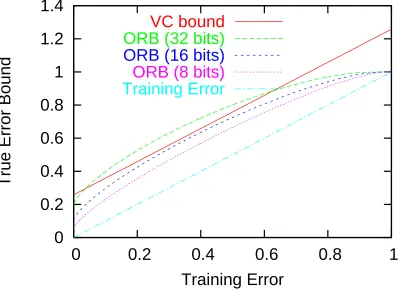
Finite class analysis is also useful in a more practical sense. In practice a finite VC dimension class usually has a finite parameterization. Given that these real parameters are typically represented as 32 bit floating point numbers, the class becomes finite and the log of the class size is linear in the number of parameters. Since many of the more sophisticated infinite-class techniques are loose by large multiplicative constants, a finite class analysis applied to a VC class discretized to a small number of bits can actually yield tighter bounds as shown in Figure 1.

2. Mathematical Preliminaries

For an arbitrary measure on an arbitrary sample space we use the notation1 ∀δSΦ[S,δ]to mean

that with probability at least 1−δover the choice of the sample S we have that Φ[S,δ]holds. In practice S is the training sample of a learning algorithm. Note that∀x∀δSΦ[x,S,δ]does not imply ∀δS∀xΦ[x,S,δ]. If X is a finite set, and for all x∈X we have the assertion∀δ>0∀δSΦ[S,x,δ]then by a standard application of the union bound we have the assertion∀δ>0∀δS∀x∈XΦ[S,x,_|X|δ ]. We call this the quantification rule. If∀δ>0∀δSΦ[S,δ]and∀δ>0∀δSΨ[S,δ]then by a standard application of the union bound we have∀δ>0∀δSΦ[S,δ₂]∧Ψ[S,δ₂]. We call this the conjunction rule.

The KL-divergence of p from q, denoted D(q||p), is q ln(q_p) + (1−q)ln(1₁−q_−p)with 0 ln(0

p) =0

and q ln(q₀) =∞. Let ˆp be the fraction of heads in a sequence S of m tosses of a biased coin where

(4)

0

0.2

0.4

0.6

0.8

1

1.2

1.4

0

0.2

0.4

0.6

0.8

1 True Error Bound

Training Error

VC bound

ORB (32 bits)

ORB (16 bits)

ORB (8 bits)

Training Error

Figure 1: A graph comparing the (infinite hypothesis) VC bound to the finite hypothesis Occam’s

razor bound. For all curves we use VC dimension d=10, bound failure probability,δ=

0.1, and m=1000 examples. For the VC bound calculation (see Moore, 2004, for details)

the formula is true error≤train error+

q

(d ln2m_d +ln4_δ)/m. For the Occam’s Razor Bound (see Langford, 2003, for details) calculation, we use a uniform distribution over

the 2kd_{discrete classifiers which might be representable when we discretize d parameters}

(5)

the probability of heads is p. We have the following inequality given by Chernoff (1952):

∀q∈[p,1]: Pr(pˆ≥q) ≤ e−mD(q||p). (1)

This bound can be rewritten as follows:

∀δ>0∀δS D(max(pˆ,p)||p)≤ ln( 1

δ)

m . (2)

To derive (2) from (1) note that Pr(D(max(pˆ,p)||p)≥ ln(1δ)

m )equals Pr(pˆ≥q)where q≥ p and

D(q||p) =ln(1δ)

m . By (1) we then have that this probability is no larger than e−mD(q||p)=δ. It is just

as easy to derive (1) from (2) so the two statements are equivalent. By duality, i.e., by considering

the problem defined by replacing p by 1−p, we get

∀δ>0∀δS D(min(pˆ,p)||p)≤ln( 1

δ)

m . (3)

Conjoining (2) and (3) yields the following corollary of (1):

∀δ>0∀δS D(pˆ||p)≤ln( 2

δ)

m . (4)

Using the inequality D(q||p)≥2(q−p)2_{one can show that (4) implies the better known form of} the Chernoff bound

∀δ>0∀δS |p−pˆ| ≤

s ln(2_δ)

2m . (5)

Using the inequality D(q||p)≥ (p−q_2q)2, which holds for q≤ p, we can show that (3) implies the following:2

∀δ>0∀δS p≤pˆ+

s 2 ˆp ln(1

δ)

m +

2 ln(1

δ)

m . (6)

Note that for small values of ˆp formula (6) gives a tighter upper bound on p than does (5). The

upper bound on p implicit in (4) is somewhat tighter than the minimum of the bounds given by (5) and (6).

We now consider a formal setting for hypothesis learning. We assume a finite set

H

of

hypothe-ses and a space

X

of instances. We assume that each hypothesis represents a function from

X

to

{0,1}where we write h(x)for the value of the function represented by hypothesis h when applied to instance x. We also assume a distribution D on pairshx,yi with x∈

X

and y∈ {0,1}. For any hypothesis h we define the error rate of h, denoted e(h), to be P_h_x_,_y_i_∼D(h(x)6=y). For a given

sample S of m pairs drawn from D we write ˆe(h)to denote the fraction of the pairshx,yiin S such that h(x)6=y. Quantifying over h∈

H

in (4) yields the following second corollary of (1):

∀δS ∀h∈

H

D(eˆ(h)||e(h))≤ln|

H

|+ln( 2

δ)

m . (7)

(6)

By considering bounds on D(q||p)we can derive the more well known corollary of (7),

∀δS ∀h∈

H

|e(h)−eˆ(h)| ≤

s

ln|

H

|+ln(2

δ)

2m . (8)

These two formulas both limit the distance between ˆe(h)and e(h). In this paper we work with (7) rather than (8) because it yields an (implicit) upper bound on generalization error that is optimal up to asymptotic equality.

3. The Upper Bound

Our goal now is to improve on (7). Our first step is to divide the hypotheses in

H

into m disjoint

sets based on their true error rates. More specifically, for p∈[0,1]defineddpeeto be max(1_m,dmpe). Note thatddpeeis of the form _mk where either p=0 and k=1 or p>0 and p∈(k−1

m , k

m]. In either

case we haveddpee ∈ {1

m, . . . , m

m}and ifddpee= k

m then p∈[

k−1

m , k

m]. Now we define

H

( k m)to be

the set of h∈

H

such thatdde(h)ee= k

m. We define s( k

m)to be ln(max(1,|

H

( k

m)|)). We now have

the following lemma.

Lemma 3.1 With high probability over the draw of S, for all hypotheses, the deviation between the empirical error ˆe(h), and true error e(h), of every hypothesis is bounded by s(dde(h)ee). More precisely,

∀δ>0∀δS ∀h∈

H

,

D(eˆ(h)||e(h))≤s(dde(h)ee) +ln( 2m

δ )

m .

Proof Quantifying over p∈ {_m1, . . . , m_m}and h∈

H

(p)in (4) gives∀δ>0,∀δS,∀p∈ {_m1, . . . , m_m}, ∀h∈

H

(p),

D(eˆ(h)||e(h))≤ ln s(p) +ln( 2m

δ )

m .

But this implies the lemma.

Lemma 3.1 imposes a constraint, and hence a bound, on e(h). More specifically, we have the

following wherelub{x : Φ[x]}denotes the least upper bound (the maximum) of the set{x : Φ[x]}:

e(h)≤lub{q : D(eˆ(h)||q)≤s(ddqee) +ln( 2m

δ )

m }. (9)

This is our uncomputable bound. It is uncomputable because the m numbers s(_m1), . . ., s(m_m) are unknown. Ignoring this problem, however, we can see that this bound is typically significantly tighter than (7). More specifically, we can rewrite (7) as

e(h)≤lub{q : D(eˆ(h)||q)≤ln|

H

|+ln( 2

δ)

m }. (10)

Since s(_mk)≤ln|

H

|, and since ln m_m is small for large m, we have that (9) is never significantly looser

(7)

(10), is significantly less than 1/2. Assuming m is large, the bound given by (9) must also be significantly less than 1/2. But for q significantly less than 1/2 we typically have that s(ddqee)is

significantly smaller than ln|

H

|. For example, suppose

H

is the set of all decision trees of size

m/10. For large m, a random decision tree of this size has error rate near 1/2. The set of decision

trees with error rate significantly smaller than 1/2 is an exponentially small fraction of the set of all possible trees. So for q small compared to 1/2 we get that s(ddqee)is significantly smaller than ln|H|. This makes the bound given by (9) significantly tighter than the bound given by (10).

We now show that the distribution of true errors can be replaced, essentially, by the histogram of training errors. We first introduce the following definitions:

ˆ

H

k

m,δ

≡

 



h∈

H

: ˆ e(h)− k

m ≤ 1 m+ s ln(16m2

δ )

2m−1

   , ˆ s k m,δ

≡ ln

max

1,2 ˆ

H

k

m,δ .

The definition of ˆs _mk,δ

is motivated by the following lemma.

Lemma 3.2 With high probability over the draw of S, for all q, s(q)≤sˆ(q,2δ). More precisely, ∀δ>0,∀δS,∀q∈ {1

m, . . . , m m},

s(q)≤sˆ(q,2δ).

Before proving Lemma 3.2 we note that by conjoining (9) and Lemma 3.2 we get the following. This is our main result.

Theorem 3.3 With high probability over the draw of S, for all hypotheses, the deviation between the empirical error ˆe(h), and true error e(h), of every hypothesis is bounded by ˆs(ddqee,δ). More precisely,

∀δ>0,∀δS,∀h∈

H

,

e(h)≤lub

(

q : D(eˆ(h)||q)≤sˆ(ddqee,δ) +ln( 4m

δ )

m

)

.

As for Lemma 3.1, the bound implicit in Theorem 3.3 is typically significantly tighter than the bound in (7) or its equivalent form (10). The argument for the improved tightness of Theorem 3.3 over (10) is similar to the argument for (9). More specifically, consider a hypothesis h for which the bound in (10) is significantly less than 1/2. Since ˆs(ddqee, δ)≤ln|

H

|, the set of values of q satisfying the condition in Theorem 3.3 must all be significantly less than 1/2. But for large m we

have that q

ln(16m2_/δ₎

2m−1 is small. So if q is significantly less than 1/2 then all hypotheses in ˆ

H

(ddqee,δ) have empirical error rates significantly less than 1/2. But for most hypothesis classes, e.g., decision trees, the set of hypotheses with empirical error rates far from 1/2 should be an exponentially small fraction of the class. Hence we get that ˆs(ddqee,δ)is significantly less than ln|

H

|and Theorem 3.3 is tighter than (10).

(8)

Lemma 3.4 (McAllester 99) For any measure on any hypothesis class we have the following where

Ehf(h)denotes the expectation of f(h)under the given measure on h:

∀δ>0∀δS Ehe(2m−1)(eˆ(h)−e(h)) 2

≤4m

δ .

Intuitively, this lemma states that with high confidence over the choice of the sample most hypotheses have empirical error near their true error. This allows us to prove that ˆs(ddqee, δ)

bounds s(ddqee). More specifically, by considering the uniform distribution on

H

(k

m), Lemma 3.4

implies

E_h∼_H₍k m)

e(2m−1)(eˆ(h)−e(h))2 ≤ 4m

δ

Pr_h∼_H₍k m)

e(2m−1)(eˆ(h)−e(h))2≥8m

δ

≤ 1

2

Pr_h∼_H₍k m)

e(2m−1)(eˆ(h)−e(h))2≤8m

δ ≥ 1 2   

h∈

H

(k

m): |eˆ(h)−e(h)| ≤ s

ln(8m

δ )

2m−1

   ≥ 1

2|

H

( k m)|

  

h∈

H

(k

m): |eˆ(h)− k m| ≤

1 m+

s ln(8m

δ )

2m−1

   ≥ 1

2|

H

( k m)|

H

(k m) ≤2 ˆ

H

k

m,2mδ

.

Lemma 3.2 now follows by quantification over q∈ {_m1, . . . , m_m}. 4. Asymptotic Analysis and Phase Transitions

This section and the two that follow give an asymptotic analysis of the bounds presented earlier. The asymptotic analysis is stated in Theorem 4.1 and Statement 6.1. To develop the asymptotic analysis, however, a preliminary discussion is needed regarding the phenomenon of phase transitions. The bounds given in (9) and Theorem 3.3 exhibit phase transitions. More specifically, the bounding

expression can be discontinuous in δ and m, e.g., arbitrarily small changes in δ can cause large

changes in the bound. To see how this happens consider the constraint on the quantity q:

D(eˆ(h)||q)≤s(ddqee) +ln( 2m

δ )

m . (11)

The bound given by (9) is the least upper bound of the values of q satisfying (11). Assume that m is sufficiently large that we can think of s(ddqee_m )as a continuous function of q which we write as ¯s(q). We can then rewrite (11) whereλis a quantity not depending on q and ¯s(q)does not depend onδ:

(9)

For q≥eˆ(h)we know that D(eˆ(h)||q)is a monotonically increasing function of q. It is reasonable

to assume that for q≤1/2 we also have that ¯s(q) is a monotonically increasing function of q.

But even under these conditions it is possible that the feasible values of q, i.e., those satisfying

(12), can be divided into separated regions. Furthermore, increasing λ can cause a new feasible

region to come into existence. When this happens the bound, which is the least upper bound of the feasible values, can increase discontinuously. At a more intuitive level, consider a large number of high error concepts and smaller number of lower error concepts. At a certain confidence level the high error concepts can be ruled out. But as the confidence requirement becomes more stringent suddenly (and discontinuously) the high error concepts must be considered. A similar discontinuity can occur in sample size. Phase transitions in shell decomposition bounds are discussed in more detail by Haussler et al. (1996).

Phase transitions complicate asymptotic analysis. But asymptotic analysis illuminates the nature of phase transitions. As mentioned in the introduction, in the asymptotic analysis of learning theory

bounds it is important that one does not hold

H

fixed as the sample size increases. If we hold

H

fixed then lim_m→∞ln|_mH|=0. But this is not what one expects for large samples in practice. As the sample size increases one typically uses larger hypothesis classes. Intuitively, we expect that even for very large m we have that ln|_mH| is far from zero.

For the asymptotic analysis of the bound in (9) we assume an infinite sequence of hypothesis classes

H

1,

H

2,

H

3 . . . and an infinite sequence of data distributions D1, D2, D3, . . .. Let sm(_mk)

be s(k

m)defined relative to

H

mand Dm. In the asymptotic analysis we assume that the sequence of

functions sm(ddqee)

m , viewed as functions of q∈[0,1], converge uniformly to a continuous function

¯s(q). This means that for anyε>0 there exists a k such that for all m>k we have

∀q∈[0,1] |sm(ddqee)

m −¯s(q)| ≤ε.

Given the functions sm(ddpee)

m and their limit function ¯s(p), we define the following functions of an

empirical error rate ˆe:

Bm(eˆ) ≡ lub

(

q : D(eˆ||q)≤sm(ddqee) +ln( 2m

δ )

m

)

,

B(eˆ) ≡ lub{q : D(eˆ||q)≤ ¯s(q)}.

The function Bm(eˆ)corresponds directly to the upper bound in (9). The function B(eˆ)is intended

to be the large m asymptotic limit of Bm(eˆ). However, phase transitions complicate asymptotic

analysis. The bound B(eˆ) need not be a continuous function of ˆe. A value of ˆe where the bound

B(eˆ) is discontinuous corresponds to a phase transition in the bound. At a phase transition the

sequence Bm(eˆ)need not converge. Away from phase transitions, however, we have the following

theorem.

Theorem 4.1 If the bound B(eˆ)is continuous at the point ˆe (so we are not at a phase transition), and the functions (parameterized by m) sm(ddqee)

m , viewed as functions of q∈[0,1], converge uniformly to

a continuous function ¯s(q), then we have

lim

(10)

Proof Define the set Fm(eˆ)as

Fm(eˆ)≡

(

q : D(eˆ||q)≤ sm(ddqee) +ln( 2m

δ )

m

)

.

This gives

Bm(eˆ) =lubFm(eˆ).

Similarly, define F(eˆ,ε)and B(eˆ,ε)as

F(eˆ,ε) ≡ {q∈[0,1]: D(eˆ||q)≤ ¯s(q) +ε}.

B(eˆ,ε) ≡ lubF(eˆ,ε).

We first show that the continuity of B(eˆ)at the point ˆe implies the continuity of B(eˆ,ε)at the pointheˆ,0i. We note that there exists a continuous function f(eˆ,ε)with f(eˆ,0) =e and such thatˆ

for anyεsufficiently near 0 we have

D(f(eˆ,ε)||q) =D(eˆ||q)−ε.

We then have

B(eˆ,ε) =B(f(x,ε)).

Since f is continuous, and B(eˆ)is continuous at the point ˆe, we get that B(eˆ,ε)is continuous at the pointheˆ,0i.

We now prove the lemma. The functions of the form sm(ddqee)+ln

2m δ

m converge uniformly to the

function ¯s(q). This implies that for anyε>0 there exists a k such that for all m>k we have

F(eˆ,−ε)⊆Fm(eˆ)⊆F(eˆ,ε).

But this in turn implies that

B(eˆ,−ε)≤Bm(eˆ)≤B(eˆ,ε). (13)

The lemma now follows from the continuity of the function B(eˆ,ε)at the pointheˆ,0i.

Theorem 4.1 can be interpreted as saying that for large sample sizes, and for values of ˆe other

than the special phase transition values, the bound has a well defined value independent of the

confidence parameterδand determined only by a smooth function ¯s(q). A similar statement can be

made for the bound in Theorem 3.3 — for large m, and at points other than phase transitions, the

bound is independent ofδand is determined by a smooth limit curve.

For the asymptotic analysis of Theorem 3.3 we assume an infinite sequence

H

1,

H

2,

H

3,. . .of

hypothesis classes and an infinite sequence S1, S2, S3,. . .of samples such that sample Smhas size

m. Let

H

m(_mk,δ)and ˆsm(_mk,δ)be

H

(_mk,δ)and ˆs(_mk,δ)respectively defined relative to hypothesis

class

H

m and sample Sm. Let Um(_mk) be the set of hypotheses in

H

m having an empirical error of

exactly _mk in the sample Sm. Let um(_mk) be ln(max(1,|Um(_mk)|). In the analysis of Theorem 3.3

we allow that the functions um(ddqee)

m are only locally uniformly convergent to a continuous function

¯u(q), i.e., for any q∈[0,1]and anyε>0 there exists an integer k and real numberγ>0 satisfying

∀m>k,∀p∈(q−γ,q+γ)|um(ddpee)

(11)

Theorem 4.2 If the functions um(ddqee)

m converge locally uniformly to a continuous function ¯u(q)

then, for any fixed value ofδ, the functions sˆm(ddqee,δ)

m also converge locally uniformly to ¯u(q). If the

convergence of um(ddqee)

m is uniform, then so is the convergence of

ˆ

sm(ddqee,δ)

m .

Proof Consider an arbitrary value q∈[0,1]andε>0. We construct the desired k andγ. More specifically, select k sufficiently large andγsufficiently small that we have the properties

∀m>k,∀p∈(q−2γ,q+2γ)

um(ddpee)

m −¯u(p) <ε 3,

∀p∈(q−2γ,q+2γ) |¯u(p)−¯u(q)| ≤ε 3,

1 k+

s ln(16k2

δ )

2k−1 <γ,

ln k k ≤

ε

3.

Consider an m>k and p∈(q−γ,q+γ). It now suffices to show that

ˆ

sm(ddpee,δ)

m −¯u(p)

≤ε.

Because Um(ddpee)is a subset of

H

m(ddpee,δ)we have

ˆ

sm(ddpee,δ)

m ≥

um(ddpee)

m ≥ ¯u(p)−

ε

3.

We can also upper bound sˆm(ddpee,δ)

m as follows:

|

H

m(ddpee,δ)| ≤

∑

|k m−p|≤γ Um k m ≤

∑

|k m−p|≤γ

eum(mk)

≤

∑

|k m−p|≤γ

em(u¯(mk)+ε3)

≤

∑

|k m−p|≤γ

em(u¯(p)+2ε3)

≤ mem(u¯(p)+2ε3)

ˆ

s(ddpee,δ)

m ≤ ¯u(p) + 2ε

3 +

ln m m

(12)

A similar argument shows that if um(ddqee)

m converges uniformly to ¯u(q)then so does

um(ddqee)

m .

Given quantities sˆi(ddqee,δ)

m that converge uniformly to ¯u(q)the remainder of the analysis is

iden-tical to that for the asymptotic analysis of (9). We define the upper bounds

ˆ

Bm(eˆ) ≡ lub

(

q : D(eˆ||q)≤sˆm(ddqee,δ) +ln 4m

δ

m

)

.

ˆ

B(eˆ) ≡ lub{q : D(eˆ||q)≤ ¯u(q)}.

Again we say that ˆe is at a phase transition if the function ˆB(eˆ)is discontinuous at the value ˆe. We then get the following whose proof is identical to that of Theorem 4.1.

Theorem 4.3 If the bound ˆB(eˆ)is continuous at the point ˆe (so we are not at a phase transition), and the functions um(ddqee)

m converge uniformly to ¯u(q), then we have that

lim

m→∞Bˆm(eˆ) =Bˆ(eˆ).

5. Asymptotic Optimality of (9)

Formula (9) can be viewed as providing an upper bound on e(h) as a function of ˆe(h) and the

function s. In this section we show that for any curve s and value ˆe there exists a hypothesis class and data distribution such that the upper bound in (9) is realized up to asymptotic equality. Up to

asymptotic equality, (9) is the tightest possible bound computable from ˆe(h) and the m numbers

s(1

m),. . ., s( m m).

The classical VC dimensions bounds are nearly optimal over bounds computable from the cho-sen hypothesis error rate ˆe(h∗)and the class

H

. The m numbers s(1

m),. . ., s( m

m)depend on both

H

and the data distribution. Hence the bound in (9) uses information about the distribution and hence can be tighter than classical VC bounds. A similar statement applies to the bound in Theorem (3.3)

computed from the empirically observable numbers ˆs(1

m), . . ., ˆs( m

m). In this case, the bound uses

more information from the sample than just ˆe(h). The optimality theorem given here also differs

from the traditional lower bound results for VC dimension in that here the lower bounds match the upper bounds up to asymptotic equality.

The departure point for our optimality analysis is the following lemma from Cover and Thomas (1991).

Lemma 5.1 (Cover and Thomas) If ˆp is the fraction of heads out of m tosses of a coin where the true probability of heads is p then for q≥p we have

Pr(pˆ≥q)≥ 1 m+1e

−mD(q||p)_.

This lower bound on Pr(pˆ≥q)is very close to Chernoff’s 1952 upper bound (1). The tightness of (9) is a direct reflection of the tightness (1). To exploit Lemma 5.1 we need to construct hypothesis classes and data distributions where distinct hypotheses have independent training errors. More specifically, we say that a set of hypotheses {h1, . . . , hn} has independent training errors if the

(13)

By an argument similar to the derivation of (3) from (1) we can prove the from Lemma 5.1 that

Pr D(min(pˆ,p)||p)≥ ln( 1

δ)−ln(m+1)

m

!

≥δ. (14)

Lemma 5.2 Let X be any finite set, S a random variable, andΘ[S,x,δ]a formula such that for every x∈X andδ>0 we have Pr(Θ[S,x,δ])≥δ, and Pr(∀x∈XΘ[S,x,δ]) =∏_x∈XPr(Θ[S,x,δ]). We then have∀δ>0∀δS ∃x∈X Θ[S,x,ln(1δ)

|X| ].

Proof

Pr(Θ[S,x,ln(1δ)

|X| ]) ≥

ln(1 δ) |X|

Pr(¬Θ[S,x,ln( 1 δ)

|X| ]) ≤ 1−

ln(1 δ) |X|

≤ e−

ln(1 δ) |X|

Pr(∀x∈X¬Θ[S,x,ln( 1 δ)

|X| ]) ≤ e−

ln(1 δ)₌δ_.

Now define h∗(k

m)to be the hypothesis of minimal training error in the set

H

( k

m). Letglb{x :

Φ[x]} denote the greatest lower bound (the minimum) of the set {x : Φ[x]}. We now have the

following lemma.

Lemma 5.3 If the hypotheses in the class

H

(ddqee) are independent then ∀δ>0, ∀δS, ∀q∈ {1

m, . . . , m m},

ˆ

e(h∗(q))≤glb

n ˆ

e : D(min(eˆ,q−1

m)||q)≤

s(q)−ln(m+1)−ln(ln(m

δ)) m

o

.

Proof To prove Lemma 5.3 let q be a fixed rational number of the form _mk. Assuming independent hypotheses we can applying Lemma 5.2 to (14) to get∀δ>0,∀δS,∃h∈

H

(k

m),

D(min(eˆ(h),e(h))||e(h))≥ s(q)−ln(m+1)−ln(ln( 1

δ))

m

Let w be the hypothesis in

H

(q)satisfying this formula. We now have ˆe(h∗(q))≤eˆ(w)and q−1

m≤

e(w)≤q. These two conditions imply∀δ>0,∀δS,

D(min(eˆ(h∗(q)),q−_m1)||q)≥s(q)−ln(m+1)−ln(ln 1 δ)

m .

This implies that

ˆ

e(h∗(q))≤glb

n ˆ

e : D(min(eˆ,q−1

m)||q)≤

s(q)−ln(m+1)−ln(ln(1 δ))

m .

o

Lemma 5.3 now follows by quantification over q∈ {1

(14)

For q∈[0,1]we have that Lemma 3.1 implies that

ˆ

e(h∗(ddqee))≥glb

n ˆ

e : D ˆe||ddqee −1

m

≤s(ddqee)+ln(2mδ )

m .

o

We now have upper and lower bounds on the quantity ˆe(h∗(ddqee))which agree up to asymptotic equality — in a large m limit where sm(ddqee)

m converges (pointwise) to a continuous function ¯s(q)we

have that the upper and lower bound on ˆe(h∗(ddqee))both converge (pointwise) to

ˆ

e(h∗(q)) =glb{e : Dˆ (eˆ||q)≤¯s(q)}.

This asymptotic value of ˆe(h∗(q))is a continuous function of q. Since q is held fixed in calculating the bounds on ˆe(ddqee), phase transitions are not an issue and uniform convergence of the functions

sm(ddqee)

m is not required. Note that for large m and independent hypotheses we get that ˆe(h

∗₍_q₎₎_is

determined as a function of the true error rate q and s(ddqee_m ).

The following lemma states that any limit function ¯s(p) is consistent with the possibility that

hypotheses are independent. This, together with Lemma 5.3 implies that no uniform bound on e(h)

as a function of ˆe(h)and|

H

(1

m)|,. . .,|

H

( m

m)|can be asymptotically tighter than (9).

Theorem 5.4 Let ¯s(p)be any continuous function of p∈[0,1]. There exists an infinite sequence of hypothesis spaces

H

1,

H

2,

H

3,. . ., and sequence of data distributions D1, D2, D3,. . .such that each class

H

m has independent hypotheses for data distribution Dm and such that sm(ddpee_m ) converges

(pointwise) to ¯s(p).

Proof First we show that if|

H

m(_mi)|=em ¯s(

i

m)then the functions sm(ddpee)

m converge (pointwise) to

¯s(p). Assume|

H

m(_mi)|=em ¯s(

i

m). In this case we have

sm(ddpee)

m =¯s(ddpee).

Since ¯s(p)is continuous, for any fixed value of p we get thatsm(ddpee)

m converges to ¯s(p).

Recall that Dmis a probability distribution on pairshx,yiwith y∈ {0,1}and x∈Xmfor some

set Xm. We take

H

m to be a disjoint union of sets

H

m(_mk) where |

H

m(_mk)| is selected as above.

Let f1, . . ., fN be the elements of

H

m with N=|

H

m|. Let Xm be the set of all N-bit bit strings

and define fi(x) to be the value of ith bit of the bit vector x. Now define the distribution Dm on

pairshx,yiby selecting y to be 1 with probability 1/2 and then selecting each bit of x independently where the ith bit is selected to disagree with y with probability _mk where k is such that fi∈

H

m(_mk).

6. Relating ˆs and s

In this section we show that in large m limits of the type discussed in Section 4 the histogram of empirical errors need not converge to the histogram of true errors. So even in the large m asymptotic limit, the bound given by Theorem 3.3 is significantly weaker than the bound given by (9).

(15)

sequence of hypothesis spaces

H

1,

H

2,

H

3,. . .and an infinite sequence of data distributions D1, D2, D3,. . .using the construction in the proof of Theorem 5.4. We note that if ¯s(p)is differentiable with bounded derivative then the functions sm(ddpee)

m converge uniformly to ¯s(p).

For a given infinite sequence data distributions we generate an infinite sample sequence S1, S2, S3,. . ., by selecting Smto consists of m pairs hx,yidrawn IID from distribution Dm. For a given

sample sequence and h∈

H

mwe define ˆem(h)and ˆsm(_mk,δ)in a manner similar to ˆe(h)and ˆs(_mk,δ)

but for sample Sm. The main result of this section is the following.

Conjecture 6.1 If each

H

mhas independent hypotheses under data distribution Dm, and the

func-tions sm(ddpee)

m converge uniformly to a continuous function ¯s(p), then for anyδ>0 and p∈[0,1],

we have, with probability 1 over the generation of the sample sequence, that

lim

m→∞

ˆ

sm(ddpee,δ)

m =_q∈sup_[₀_,₁_]¯s(q)−D(p||q).

We call this a conjecture rather than a theorem because the proof has not been worked out to a high level of rigor. Nonetheless, we believe the proof sketch given below can be expanded to a fully rigorous argument.

Before giving the proof sketch we note that the limiting value of sˆm(ddpee,δ)

m is independent ofδ.

This is consistent with Theorem 4.2. Define

¯_ˆ

s(p)≡ sup

q∈[0,1]

¯s(q)−D(p||q).

Note that ¯sˆ(p)≥ ¯s(p). This gives an asymptotic version of Lemma 3.2. But since D(p||q)can be locally approximated as c(p−q)2_{(up to its second order Taylor expansion), if ¯}_s₍_p₎_{is increasing at} the point p then we also get that ¯sˆ(p)is strictly larger than ¯s(p).

Proof Outline: To prove Statement 6.1 we first define

H

m(p, q)for p,q∈ {_m1, . . . , m_m}to be

the set of all h∈

H

m(q)such that ˆem(h) =p. Intuitively,

H

m(p,q)is the set of concepts with true

error rate near q that have empirical error rate p. Ignoring factors that are only polynomial in m, the probability of a hypothesis with true error rate q having empirical error rate p can be written as (approximately) e−mD(p||q). So the expected size of

H

m(p, q)can be written as|

H

m(q)|e−mD(p||q),

or alternatively, (approximately) as em ¯s(q)e−mD(p||q)or em(s¯(q)−D(p||q)). More formally, we have, for any fixed value of p and q,

lim

m→∞

ln(max(1,E(|

H

m(ddpee,ddqee)|)))

m

=max(0, ¯s(q)−D(p||q)).

We now show that the expectation can be eliminated from the above limit. First, consider distinct values of p and q such that ¯s(q)−D(p||q)>0. Since p and q are distinct, the probability that a fixed hypothesis in

H

m(ddqee) is in

H

m(ddpee, ddqee) declines exponentially in m. Since

¯s(q)−D(p||q)>0 the expected size of

H

m(ddpee, ddqee) grows exponentially in m. Since the

hypotheses are independent, the distribution of possible values of |

H

m(ddpee, ddqee)| becomes

essentially a Poisson mass distribution with an expected number of arrivals growing exponentially in m. The probability that|

H

m(ddpee,ddqee)|deviates from its expectation by as much as a factor

(16)

have that|

H

m(ddpee,ddqee)|is within a factor of 2 of its expectation. Since the probability of being

unsafe at m declines exponentially in m, for anyδthere exists a k such that with probability at least

1−δthe sample sequence is safe after k. So for any δ>0 we have that with probability at least

1−δthe sequence is safe after some k. But since this holds for allδ>0, with probability 1 such a k must exist:

lim

m→∞

ln(max(1,|

H

m(ddpee,ddqee)|))

m

=¯s(q)−D(p||q).

We now define

sm(ddpee,ddqee)≡ln(max(1,|

H

m(ddpee,ddqee)|)).

It is also possible to show for p=q we have that with probability 1 we have that sm(ddpee,ddqee)

m

approaches ¯s(p) and that for distinct p and q with ¯s(q)−D(p||q)≤0 we have thatsm(ddqee,ddqee)

m

approaches 0. Putting these together yields that, with probability 1, we have

lim

m→∞

sm(ddpee,ddqee)

m =max(0, ¯s(q)−D(p||q)). (15)

Define Um(_mk)and um(_mk)as in Section 4. We now have the following equality:

Um(p) =∪_q∈{1

m, ...,mm}

H

m(p,q).

We now show that with probability 1, um(p)

m approaches ¯sˆ(p). First, consider a p∈[0,1] such

that ¯sˆ(p)>0. Let Since ¯s(q)−D(q||p) is a continuous function, and [0,1] is a compact set, sup_q∈_[₀_,₁_]¯s(q)−D(p||q) must be realized at some value q∗ ∈[0,1]. Let q∗ be such that ¯s(q∗)− D(p||q∗) equals ¯sˆ(p). We have that um(ddpee) ≥sm(ddpee, ddq∗ee). This, together with (15),

implies that

lim inf

m→∞

um(ddpee)

m ≥s¯ˆ(p).

The sample sequence is “safe” at m and _mk if|

H

m(ddpee,dd_mkee)|does not exceed twice the

expec-tation of|

H

m(ddpee, ddq∗ee)|. Assuming uniform convergence of sm(ddpee_m ), the probability of not

being safe at m and _mk declines exponentially in m at a rate at least as fast as the rate of decline of the probability of not being safe at m andddq∗ee. By the union bound this implies that for a given m

the probability that there exists an unsafe _mk also declines exponentially. We say that the sequence

is safe after N if it is safe for all m and _mk with m>N. The probability of not being being safe after N also declines exponentially with N. By an argument similar to that given above, this implies that with probability 1 over the choice of the sequence there exists a N such that the sequence is safe after N. But if we are safe at m then|Um(ddpee)| ≤2mE|

H

m(p,ddq∗ee)|. This implies that

lim sup

m→∞

um(ddpee)

m ≤¯sˆ(p).

Putting the two bounds together we get

lim

m→∞

um(ddpee)

(17)

The above argument establishes (to some level of rigor) pointwise convergence of um(ddpee)

m to

¯_ˆ

s(p). It is also possible to establish a convergence rate that is a continuous function of p. This implies that the convergence of um(ddpee)

m can be made locally uniform. Theorem 4.2 then implies

the desired result.

7. Improvements

Theorem 3.3 has been improved in various ways (Langford, 2002):

• Removing the discretization of true errors,

• Using one-sided bounds,

• Using nonuniform union bounds over discrete values of the form _mk,

• Tightening the Chernoff bound using direct calculation of Binomial coefficients, and

• Improving Lemma 3.4.

These improvements allow the removal of all but one ln(m)terms from the statement of the bound.

However, they do not improve the asymptotic equations given by Theorem 4.1 and Statement 6.1. A practical difficulty with the bound in Theorem 3.3 is that it is usually impossible to enumer-ate the elements of an exponentially large hypothesis class and hence impractical to compute the histogram of training errors for the hypotheses in the class. In practice the values of s(k

m)might be

estimated using some form of Monte-Carlo Markov chain sampling over the hypotheses. For certain hypothesis spaces it might also be possible to directly calculate the empirical error distribution with-out evaluating every hypothesis. For example, this can be done with “partition rules” which, given a fixed partition of the input space, make predictions which are constant on each partition. If there are n elements in the partition then there are 2npartition rules. For a fixed partition, the histogram of

empirical errors for the 2npartition rules can be computed in polynomial time. Note that the class

of decision trees is a union of partition rules where the structure of a tree defines a partition and the labels at the leaves of the tree define a particular partition rule relative to that partition. Taking advantage of this, it is suprisingly easy to compute a shell bound for small decision trees (Langford, 2002).

8. Discussion and Conclusion

(18)

One of the goals of learning theory is to give generalization guarantees that are predictive of actual generalization error. It is well known that the actual generalization error can exhibit phase transitions — as the sample size increases the expected generalization error can jump essentially discontinuously in sample size. So accurate true error bounds should also exhibit phase transitions. Shell bounds exhibit these phase transitions while other bounds such as VC dimension results do not.

The phase transitions can also be interpreted as a statement about the bound as a function of the

confidence parameterδ. As the value ofδis varied the bound may shift essentially discontinuously.

To put this another way, let h∗be the hypothesis of minimal training error on a large sample. Near a phase transition in true generalization error (as opposed to a phase transition in the bound) we may have that with probability 1−δthe true error of h∗is near its training error but with probabilityδ/2, say, the true error of h∗can be far from its training error. More traditional bounds do not exhibit this kind of sensitivity toδ. Bounds that exhibit phase transitions seem to bring the theoretical analysis of generalization closer to the actual phenomenon.

Acknowledgments

Yoav Freund, Avrim Blum, and Tobias Scheffer all provided useful discussion in forming this paper.

References

P. Bartlett, O. Bousquet and S. Mendelson. Localized Rademacher complexities. Proceedings of the 15th Annual Conference on Computational Learning Theory, pp. 44-58, (2002).

H. Chernoff. A measure of asymptotic efficiency for test of a hypothesis based on the sum of obser-vations. Annals of Mathematical Statistics, 23:493-507, 1952.

T. M. Cover and J. A. Thomas. Elements of Information Theory, Wiley, 1991.

Y. Freund. Self bounding algorithms. Computational Learning Theory (COLT), 1998.

D. Haussler, M. Kearns, H. S. Seung, and N. Tishby. (1996). Rigorous learning curve bounds from statistical mechanics. Machine Learning 25, pp. 195-236, 1996.

J. Langford. Practical prediction theory for classification, ICML 2003 tutorial, avaliable at http://hunch.net/ jl/projects/prediction bounds/tutorial/tutorial.ps.

J. Langford. Quantitatively tight sample complexity bounds. Ph.D. Thesis, Carnegie Mellon, 2002.

J. Langford and A. Blum, Microchoice and self-bounding algorithms. Computational Learning The-ory (COLT), 1999.

Y. Mansour and D. McAllester. Generalization bounds for decision trees. Computational Learning Theory (COLT), 2000.

A. Moore. VC dimension for characterizing classifiers. Tutorial at

(19)

D. McAllester. PAC-Bayesian model averaging. Computational Learning Theory (COLT), 1999.

D. McAllester and R. Schapire. On the convergence rate of good-Turing estimators. Computational Learning Theory (COLT), 2000.

T. Scheffer and T. Joachims. Expected error analysis for model selection. International Conference on Machine Learning (ICML), 1999.