Multiclass Classification with
Multi-Prototype Support Vector Machines
Fabio Aiolli [email protected]
Alessandro Sperduti [email protected]
Dip. di Matematica Pura e Applicata Universit`a di Padova
Via G. Belzoni 7 35131 Padova, Italy
Editor: Yoram Singer
Abstract
Winner-take-all multiclass classifiers are built on the top of a set of prototypes each representing one of the available classes. A pattern is then classified with the label associated to the most ‘similar’ prototype. Recent proposal of SVM extensions to multiclass can be considered instances of the same strategy with one prototype per class.
The multi-prototype SVM proposed in this paper extends multiclass SVM to multiple proto-types per class. It allows to combine several vectors in a principled way to obtain large margin decision functions. For this problem, we give a compact constrained quadratic formulation and we propose a greedy optimization algorithm able to find locally optimal solutions for the non convex objective function.
This algorithm proceeds by reducing the overall problem into a series of simpler convex prob-lems. For the solution of these reduced problems an efficient optimization algorithm is proposed. A number of pattern selection strategies are then discussed to speed-up the optimization process. In addition, given the combinatorial nature of the overall problem, stochastic search strategies are suggested to escape from local minima which are not globally optimal.
Finally, we report experiments on a number of datasets. The performance obtained using few simple linear prototypes is comparable to that obtained by state-of-the-art kernel-based methods but with a significant reduction (of one or two orders) in response time.
Keywords: multiclass classification, multi-prototype support vector machines, kernel
ma-chines, stochastic search optimization, large margin classifiers
1. Introduction
Multiclass classifiers are often based on the winner-take-all (WTA) rule. WTA based classifiers define a set of prototypes, each associated with one of the available classes from a set
Y
. A scoring function f :X
×M
→Ris then defined, measuring the similarity of an element inX
with prototypes defined in a spaceM
. For simplicity, in the following, we assumeM
≡X
. When new instances are presented in input, the label that is returned is the one associated with the most ’similar’ prototype:H(x) =
C
arg max
r∈Ω f(x,Mr)
(1)
whereΩis the set of prototype indexes, the Mr’s are the prototypes and
C
:Ω→Y
the functionreturning the class associated to a given prototype. An equivalent definition can also be given in terms of the minimization of a distance or loss (these cases are often referred to as distance-based and loss-based decoding respectively).
1.1 Motivations and Related Work
Several well-known methods for binary classification, including neural networks (Rumelhart et al., 1986), decision trees (Quinlan, 1993), k-NN (see for example (Mitchell, 1997)), can be naturally extended to the multiclass domain and can be viewed as instances of the WTA strategy. Another class of methods for multiclass classification are the so called prototype based methods, one of the most relevant of which is the learning vector quantization (LVQ) algorithm (Kohonen et al., 1996). Although different versions of the LVQ algorithm exist, in the more general case these algorithms quantize input patterns into codeword vectors ciand use these vectors for 1-NN classification.
Sev-eral codewords may correspond to a single class. In the simplest case, also known as LVQ1, at each step of the codewords learning, for each input pattern xi, the algorithm finds the element ckclosest
to xi. If that codeword is associated to a class which is the same as the class of the pattern, then ck
is updated by ck←ck+η(t)(xi−ck)thus making the prototype get closer to the pattern, otherwise
it is updated by ck←ck−η(t)(xi−ck)thus making the prototype farther away. Other more
com-plicated versions exist. For example, in the LVQ2.1, let y be the class of the pattern, at each step the closest codeword of class c6=y and the closest codeword of class y are updated simultaneously. Moreover, the update is done only if the pattern under consideration falls in a ”window” which is defined around the midplane between the selected codewords.
When the direct extension of a binary method into a multiclass one is not possible, a general strategy to build multiclass classifiers based on a set of binary classifiers is always possible, the so called error correcting output coding (ECOC) strategy, originally proposed by Dietterich and Bakiri in (Dietterich and Bakiri, 1995). Basically, this method codifies each class of the multiclass problem as a fixed size binary string and then solves one different binary problem for each bit of the string. Given a new instance, the class whose associated string is most ’similar’ to the output of the binary classifiers on that instance is returned as output. Extensions to codes with values in
{−1,0,+1} (Allwein et al., 2000) and continuous codes (Crammer and Singer, 2000) have been recently proposed.
to the ’kernel trick’ when dot products can be computed efficiently by means of a kernel function k(x,y) =hφ(x),φ(y)idefined in terms of the original patterns. Examples of kernel functions are the polynomial kernel
k(x,y) = (hx,yi+u)d,u≥0,d∈N
of which the linear case is just an instance (d=1) and the radial basis function (RBF) kernel
k(x,y) =exp(−λ||x−y||2),λ≥0.
Kernel machines, and the SVM in particular, has been initially devised for the binary setting. However, extensions to the multiclass case have been promptly proposed (e.g. Vapnik, 1998; Weston and Watkins, 1999; Guermeur et al., 2000; Crammer and Singer, 2000).
The discriminant functions generated by general kernel-based methods are implicitly defined in terms of a subset of the training patterns, the so called support vectors, on the basis of a linear combination of kernel products f(x) =∑i∈SVαik(xi,x). In the particular case of the kernel function
being linear, this sum can be simplified in a single dot product. When this is not the case, the implicit form allows to elegantly deal with non linear decision functions obtained by using non linear kernels. In this last case, the efficiency with respect to the time spent for classifying new vectors tends to be low when the number of support vectors is large. This has motivated some recent works, briefly discussed in the following, whose aim was at building kernel-based machines with a minimal number of support vectors.
The relevance vector machine (RVM) in (Tipping, 2001) is a model used for regression and classification exploiting a probabilistic Bayesian learning framework. It introduces a prior over the weights of the model and a set of hyperparameters associated to them. The form of the RVM pre-diction is the same as the one used for SVM. Sparsity is obtained because the posterior distributions of many of the weights become sharply peaked around the zero. Other interesting advantages of the RVM are that it produces probabilistic predictions and that it can be applied to general functions and not only to kernel functions satisfying the Mercer’s condition. The minimal kernel classifier (MKC) in (Fung et al., 2002) is another model theoretically justified by linear programming pertur-bation and a bound on the leave-one-out error. This model uses a particular loss function measuring both the presence and the magnitude of an error. Finally, quite different approaches are those in (Sch¨olkopf et al., 1999; Downs et al., 2001) that try to reduce the number of support vectors after the classifiers have been constructed.
set-ting since the explicit representation for the models can be used.
In Section 2 we give some preliminaries and the notation we adopt along the paper. Then, in Section 3 we derive a convex quadratic formulation for the easier problem of learning one prototype per class. The obtained formulation can be shown to be equivalent, up to a change of variables and constant factors, to the one proposed by Crammer and Singer (2000). When multiple prototypes are introduced in Section 4, the problem becomes not convex in general. However, in Section 5 we will see that once fixed an appropriate set of variables, the reduced problem is convex. Moreover, three alternative methods are given for this optimization problem and heuristics for the ”smart” selection of patterns in the optimization process are proposed and compared. Then, in Section 6 we give a greedy procedure to find a locally optimal solution for the overall problem and we propose an ef-ficient stochastic-search based method to improve the quality of the solution. In Section 7 we give theoretical results about the generalization ability of our model. Specifically, we present an upper bound on the leave-one-out error and upper bounds on the generalization error. Finally, the experi-mental work in Section 8 compares our linear method with state-of-the-art methods, with respect to the complexity of the generated solution and with respect to the generalization error.
This paper substantially extends the material contained in other two conference papers. Namely, (Aiolli and Sperduti, 2003) which contains the basic idea and the theory of the multi-prototype SVM together with preliminary experimental work and (Aiolli and Sperduti, 2002a) which proposes and analyzes selection heuristics for the optimization of multiclass SVM.
2. Preliminaries
Let us start by introducing some definitions and the notation that will be used in this paper. We assume to have a labelled training set
S
={(x1,c1), . . . ,(xn,cn)}of cardinality n, where xi∈X
arethe examples in a inner-product space
X
⊆Rd and ci∈Y
={1, . . . ,m}the corresponding class or label. To keep the notation clearer, we focus on the linear case where kernels are not used. However, we can easily consider the existence of a feature mappingφ:I
→X
. In this case, it is trivial to extend the derivations we will obtain to non-linear mappings x7→φ(x) of possibly non vectorial patterns by substituting dot productshx,yiwith a suited kernel function k(x,y) =hφ(x),φ(y)iand the squared 2-norm ||x||2 with k(x,x) consequently. The kernel matrix K ∈Rn×n is the matrix containing the kernel products of all pairs of examples in the training set, i.e. Ki j=k(xi,xj).We consider dot-product based WTA multiclass classifiers having the form
HM(x) =
C
arg max
r∈ΩhMr,xi
(2)
whereΩis the set of prototype indices and the prototypes are arranged in a matrix M∈R|Ω|×dand
C
:Ω→Y
the function that, given an index r, returns the class associated to the r-th prototype. We also denote by yri, 1≤i≤n, r∈Ω, the constant that is equal to 1 ifC
(r) =ci and−1 otherwise.Moreover, for a given example xi,
P
i={r∈Ω: yri =1} is the set of ’positive’ prototypes for theexample xi, i.e. the set of prototype indices associated to the class of xi, while
N
i=Ω\P
i={r∈(or simply score) of the r-th prototype vector for the instance x. Finally, symbols in bold represent vectors and, as particular case, the symbol 0 represents the vector with all components set to 0.
3. Single-Prototype Multi-Class SVM
One of the most effective multi-class extension of SVM has been proposed by Crammer and Singer (2000). The resulting classifier is of the same form of Eq. (2) where each class has associated exactly one prototype, i.e.Ω≡
Y
and∀r∈Ω,C
(r) =r. The solution is obtained through the minimization of a convex quadratic constrained function. Here, we derive a formulation that, up to a change of variables, can be demonstrated to be equivalent to the one proposed by Crammer and Singer (see Aiolli and Sperduti (2002a)). This will serve to introduce a uniform notation useful for presenting the multi-prototype extension in the following sections.In multiclass classifiers based on Eq. (2), in order to have a correct classification, the prototype of the correct class is required to have a score greater than the maximum among the scores of the prototypes associated to incorrect classes. The multiclass margin for the example xiis then defined
by
ρ(xi,ci|M) =hMyi,xii −max
r6=yi
hMr,xii,
where yi such that
C
(yi) =ci, is the index of the prototype associated to the correct label for theexample xi. In the single prototype case, with no loss of generality, we consider a prototype and the
associated class indices to be coincident, that is yi=ci. Thus, a correct classification of the example
xiwith a margin greater or equal to 1 requires the condition
hMyi,xii ≥θi+1 whereθi=max
r6=yi h
Mr,xii. (3)
to be satisfied. Note that, the condition above is implied by the existence of a matrix ˆM such that
∀r6=yi, hMˆyi,xii>hMˆr,xii. In fact, the matrix M can always be obtained by an opportune
re-scaling of the matrix ˆM. With these premises, a set of examples is said to be linearly separable by a multiclass classifier if there exists a matrix M able to fulfill the above constraints for every pattern in the set.
Unfortunately, the examples in the training set can not always be separated and some exam-ples may violate the margin constraints. We consider these cases by introducing soft margin slack variablesξi≥0, one for each example, such that
ξi= [θi+1− hMyi,xii]+,
where the symbol[z]+corresponds to the soft-margin loss that is equal to z if z>0 and 0 otherwise. Note that the valueξican also be seen as an upper bound on the binary loss for the example xi, and
SVM (SProtSVM in the following) will result in:
minM,ξ,θ12||M||2+C∑
iξi
subject to:
∀i,r6=yi,hMr,xii ≤θi,
∀i, hMyi,xii ≥θi+1−ξi, ∀i, ξi≥0
(4)
where the parameter C controls the amount of regularization applied to the model.
It can be observed that, at the optimum,θiwill be set to the maximum value among the negative
scores for the instance xi(in such a way to minimize the corresponding slack variables) consistently
with Eq. (3).
The problem in Eq. (4) is convex and it can be solved in the standard way by resorting to the optimization of the Wolfe dual problem. In this case, the Lagrangian is:
L(M,ξ,θ,α,λ) = 1 2||M||
2+C∑
iξi+
∑i,r6=yiα
r
i(hMr,xii −θi)+
∑iαyii(θi+1−ξi− hMyi,xii)−
∑iλiξi
= 12||M||2−∑i,ryirαri(hMr,xii −θi)+
∑iα yi
i +∑i(C−α
yi
i −λi)ξi,
(5)
subject to the constraintsαri,λi≥0.
By differentiating the Lagrangian with respect to the primal variables and imposing the optimal-ity conditions we obtain a set of constraints that the variables have to fulfill in order to be an optimal solution:
∂L(M,ξ,θ,α,λ)
∂Mr =0 ⇔ Mr=∑iy
r iαrixi
∂L(M,ξ,θ,α,λ)
∂ξi =0 ⇔ C−αyii−λi=0⇔αyii ≤C
∂L(w,ξ,θ,α,λ)
∂θi =0 ⇔ αyii=∑r6=yiα
r i
(6)
By using the factsαyi
i = 12∑rα
r
i and||M(α)||2=∑i,j,ryriyrjαriαrjhxi,xji, substituting equalities
from Eq. (6) into Eq. (5) and omitting constants that do not change the solution, the problem can be restated as:
maxα∑i,rαri− ||M(α)||2
subject to:
∀i,r,αr
i ≥0
∀i,αyi
i =∑r6=yiα
r
i ≤C
Notice that, when kernels are used, by the linearity of dot-products, the scoring function for the r-th prototype and a pattern x can be conveniently reformulated as
fr(x) =hMr,φ(x)i= n
∑
i=1
yriαrik(x,xi).
4. Multi-Prototype Multi-Class SVM
The SProtSVM model presented in the previous section is here extended to learn more than one prototypes per class. This is done by generalizing Eq. (3) to multiple prototypes. In this setting, one instance is correctly classified if and only if at least one of the prototypes associated to the correct class has a score greater than the maximum of the scores of the prototypes associated to incorrect classes.
A natural extension of the definition for the margin in the multi-prototype case is then ρ(xi,ci|M) =max
r∈Pi
hMr,xii −max r∈Ni
hMr,xii.
and its value will result greater than zero if and only if the example xiis correctly classified.
We can now give conditions for a correct classification of an example xiwith a margin greater
or equal to 1 by requiring that:
∃r∈
P
i: hMr,xii ≥θi+1 andθi=max r∈NihMr,xii. (7)
To allow for margin violations, for each example xi, we introduce soft margin slack variables
ξr
i ≥0, one for each positive prototype, such that
∀r∈
P
i, ξri = [θi+1− hMr,xii]+.Given a pattern xi, we arrange the soft margin slack variablesξri in a vectorξi∈R|
Pi|. Let us now
introduce, for each example xi, a new vector having a number of components equal to the number of
positive prototypes for xi,πi∈ {0,1}|Pi|, whose components are all zero except one component that
is 1. In the following, we refer toπias the assignment of the pattern xito the (positive) prototypes.
Notice that the dot product hπi,ξii is always an upper bound on the binary loss for the example
xi independently from its assignment and, similarly to the single-prototype case, the average value
over the training set represents an upper bound on the empirical error.
Now, we are ready to formulate the general multi-prototype problem by requiring a set of pro-totypes of small norm and the best assignment for the examples able to fulfill the soft constraints given by the classification requirements. Thus, the MProtSVM formulation can be given as:
minM,ξ,θ,π12||M||2+C∑
ihπi,ξii
subject to:
∀i,r∈
N
i,hMr,xii ≤θi,∀i,r∈
P
i,hMr,xii ≥θi+1−ξri,∀i,r∈
P
i,ξri ≥0
∀i,πi∈ {0,1}|Pi|.
(8)
Unfortunately, this is a mixed integer problem that is not convex and it is a difficult problem to solve in general. However, as we will see in the following, it is prone to an efficient optimization procedure that approximates a global optimum. At this point, it is worth noticing that, since this formulation is itself an (heuristic) approximation to the structural risk minimization principle where the parameter C rules the trade-off between keeping the VC-dimension low and minimizing the training error, a good solution of the problem in Eq. (8), even if not optimal, can nevertheless give good results in practice. As we will see, this claim seems confirmed by the results obtained in the experimental work.
5. Optimization with Static Assignments
Let suppose that the assignments are kept fixed. In this case, the reduced problem becomes convex and it can be solved as described above by resorting to the optimization of the Wolfe dual problem. In this case, the Lagrangian is:
Lπ(M,ξ,θ,α,λ) = 1 2||M||
2+C∑
ihπi,ξii+
∑i,r∈Piα
r
i(θi+1−ξri− hMr,xii)−
∑i,r∈Piλ
r iξri+
∑i,r∈Niα
r
i(hMr,xii −θi),
(9)
subject to the constraintsαri,λr
i ≥0.
As above, by differentiating the Lagrangian of the reduced problem and imposing the optimality conditions, we obtain:
∂Lπ(M,ξ,θ,α,λ)
∂Mr =0 ⇔ Mr=∑iy
r iαrixi
∂Lπ(M,ξ,θ,α,λ)
∂ξr
i =0 ⇔ Cπ
r
i−αri−λri =0⇔αri ≤Cπri
∂Lπ(M,ξ,θ,α,λ)
∂θi =0 ⇔ ∑r∈Piα
r
i =∑r∈Niα
r i
(10)
Notice that the second condition requires the dual variables associated to (positive) prototypes not assigned to a pattern to be 0. By denoting now as yithe unique index r∈
P
isuch thatπri =1, onceusing the conditions of Eq. (10) in Eq. (9) and omitting constants that do not change the obtained solution, the reduced problem can be restated as:
maxα∑i,rαri− ||M(α)||2
subject to:
∀i,r, αr
i ≥0
∀i, αyi
i =∑r∈Niα
r
i ≤C
∀i,r∈
P
i\ {yi},αri =0.(11)
It can be trivially shown that this formulation is consistent with the formulation of the SProtSVM dual given above. Moreover, when kernels are used, the score function for the r-th prototype and a pattern x can be formulated as in the single-prototype case as
fr(x) =hMr,φ(x)i= n
∑
i=1
yriαrik(x,xi).
Thus, when patterns are statically assigned to the prototypes via constant vectorsπi, the
convex-ity of the associated MProtSVM problem implies that the optimal solution for the primal problem in Eq. (8) can be found through the maximization of the Lagrangian as in problem in Eq. (11). Assuming an equal number q of prototypes per class, the dual involves n×m×q variables which leads to a very large scale problem. Anyway, the independence of constraints among the different patterns allows for the separation of the variables in n disjoint sets of m×q variables.
In the following, we first show that the pattern related problem can be further decomposed until the solution for a minimal subset of two variables is required. This is quite similar to the SMO procedure for binary SVM. Then, a training algorithm for this problem can be defined by iterating this basic step.
5.1 The Basic Optimization Step
In this section the basic step corresponding to the simultaneous optimization of a subset of variables associated to the same pattern is presented. Let pattern xp be fixed. Since we want to enforce the
linear constraint∑r∈Npα
r
p+λp=C, λp≥0, from the second condition in Eq. (10), two elements
from the set of variables{αrp,r∈
N
p} ∪ {λp}will be optimized in pair while keeping the solution inside the feasible region. In particular, letζ1 andζ2 be the two selected variables, we restrict the updates to the formζ1←ζ1+νandζ2←ζ2−νwith optimal choices forν.In order to compute the optimal value forνwe first observe that an additive update∆Mrto the
prototype r will affect the squared norm of the prototype vector Mrof an amount
∆||Mr||2=||∆Mr||2+2hMr,∆Mri.
Then, we examine separately the two ways a pair of variables can be selected for optimization.
(Case 1) We first show how to analytically solve the problem associated to an update involving a single variableαrp, r∈
N
p and the variableαypp. Note that, sinceλp does not influence the valueof the objective function, it is possible to solve the associated problem with respect to the variable αr
pandα
yp
p in such a way to keep the constraintαypp =∑r∈Npα
r
psatisfied and afterwards to enforce
the constraintsλp=C−∑s∈Npα
s
p≥0. Thus, in this case we have:
αr
p←αrp+νandα
yp
p ←αypp+ν.
Since∆Mr=−νxp,∆Myp =νxpand∆Ms=0 for s∈ {/ r,yp}, we obtain
∆||M||2=∆||Mr||2+∆||Myp||
2=2ν2||x
p||2+2ν(fyp(xp)−fr(xp))
and the difference obtained in the Lagrangian value will be
∆L(ν) =2ν(1−fyp(xp) +fr(xp)−ν||xp||
2).
Since this last formula is concave inν, it is possible to find the optimal value when the first derivative is null, i.e.
ˆ
ν=arg max
ν ∆L(ν) =
1−fyp(xp) +fr(xp)
2||xp||2
(12)
If the values ofαrp andαyp
p, after being updated, turn out to be not feasible for the constraints
αr
p≥0 andα yp
p ≤C, we select the unique value forνsuch to fulfill the violated constraint bounds
at the limit (αrp+ν=0 orαyp
p +ν=C respectively).
(Case 2) Now, we show the analytic solution of the associated problem with respect to an update involving a pair of variablesαr1
p,αrp2such that r1,r2∈
N
pand r16=r2. Since, in this case, the update must have zero sum, we have:αr1
In this case,∆Mr1 =−νxp,∆Mr2=νxpand∆Ms=0 for s∈ {/ r1,r2}, thus
∆||M||2=∆||Mr1|| 2+∆
||Mr2|| 2=2ν2
||xp||2+2ν(fr2(xp)−fr1(xp)) leading to an Lagrangian improvement equals to
∆L(ν) =2ν(fr1(xp)−fr2(xp)−ν||xp|| 2).
Since also this last formula is concave inν, it is possible to find the optimal value
ˆ
ν=arg max
ν ∆L(ν) =
fr1(xp)−fr2(xp) 2||xp||2
(13)
Similarly to the previous case, if the values of theαr1
p andαrp2, after being updated, turn out to be
not feasible for the constraintsαr1
p ≥0 andαrp2≥0, we select the unique value forνsuch to fulfill
the violated constraint bounds at the limit (in this case, considering fr1(xp)≤fr2(xp)and thus ˆν≤0 with no loss in generality, we obtainαr1
p +ν=0 orαrp2−ν=C respectively).
Note that, when a kernel is used, the norm in the feature space can be substituted with the diago-nal component of the kernel matrix, i.e.||xp||2=k(xp,xp) =Kppwhile the scores can be maintained
in implicit form and computed explicitly when necessary.
To render the following exposition clearer, we try to compact the two cases in one. This can be done by defining the update in a slightly different way, that is, for each pair(ra,rb)∈(
P
p∪N
p)×N
pwe define:
αra
p ←αrpa+yrpaνandαrpb ←αrpb−yrpbν
and hence the improvement obtained for the value of the Lagrangian is
Vrpa,rb(ν) =2ν
1 2(y
ra
p −yrpb)−fra(xp) +frb(xp)−νk(xp,xp)
(14)
where the optimal value for theνis
ˆ ν=
1 2(y
ra
p −yrpb)−fra(xp) +frb(xp)
2k(xp,xp)
subject to the constraints
αra
p +yrpaν>0, αrpb−yrpbν>0,αyp+
1 2(y
ra
p −yrpb)ν≤C.
The basic step algorithm and the updates induced in the scoring functions are described in Figure 1 and Figure 2, respectively.
5.2 New Algorithms for the Optimization of the Dual
BasicStep(p, ra, rb)
ν= 12(yrap−yrbp)−fra(xp)+frb(xp)
2Kpp
if (αra
p +yrpaν<0) then ν=−yrpaαrpa
if (αrb
p −yrpbν<0) then ν=yrpbαrpb
if (αypp+12(yrpa−yrpb)ν>C) then ν=2 C−αypp
yrap−yrbp
returnν
Figure 1: The basic optimization step: explicit optimization of the reduced problem with two vari-ables, namelyαra
p andαrpb.
BasicUpdate(p, ra, rb,ν)
αra=αra+y
ra
pν; αrb =αrb+y
rb
pν;
fra(xp) = fra(xp) +y
ra
pνKpp; frb(xp) = frb(xp)−y
rb
pνKpp;
Figure 2: Updates done after the basic optimization step has been performed and the optimal solu-tion found. Kppdenotes the p-th element of the kernel matrix diagonal.
• a minimal subset of independent multipliers are selected
• the analytic solution of the reduced problem obtained by fixing all the variables but the ones we selected in the previous step is found.
In our case, a minimal set of two variables associated to the same example are selected at each iteration. As we showed in the last section, each iteration leads to an increase of the Lagrangian. This, together with the compactness of the feasible set guarantees the convergence of the procedure. Moreover, this optimization procedure can be considered incremental in the sense that the solution we have found at one step forms the initial condition when a new subset of variables are selected for optimization. Finally, it should be noted that for each iteration the scores of the patterns in the training set must be updated before to be used in the selection phase. The general optimization algorithm just described is depicted in Figure 3.
In the following, we present three alternative algorithms for the optimization of the problem in Eq. (11) which differ in the way they choose the pairs to optimize through the iterations, i.e. the
OptimizeOnPatternprocedure.
OptimizeStaticProblem(ϕV)
repeat
PatternSelection(p) // Heuristically choose an example p based on Eq. (14)
OptimizeOnPattern(p,ϕV)
until converge.
Figure 3: High-level procedure for the optimization of a statically assigned multi-prototype SVM. The parameterϕV is the tolerance when checking optimality in theOptimizeOnPattern
procedure.
BasicOptimizeOnPattern(p,ϕV)
Heuristically choose two indexes ra6=rbbased on Eq. (14)
ν=BasicStep(p,ra,rb)
BasicUpdate(p,ra,rb,ν)
Figure 4: SMO-like algorithm for the optimization of statically assigned multi-prototype SVM.
is fulfilled. Eq. (14) gives a natural method for the selection of the two variables involved, i.e. take the two indexes that maximize the value of that formula. Finally, once chosen two variables to optimize, the basic step in the algorithm in Figure 1 provides the optimal solution. This very general optimization algorithm will be referred to asBasicOptimizeOnPatternand it is illustrated in Figure 4.
AllPairsOptimizeOnPattern(p,ϕV)
t=0, V(0) =0.
do
t←t+1, V(t) =0
For each r16=r2
ν=BasicStep(p,r1,r2) V(t) =V(t) +2ν 12(yr1
p −yrp2)−fr1(xp) + fr2(xp)−νKpp
BasicUpdate(p,r1,r2,ν)
until (V(t)≤ϕV)
Figure 5: Algorithm for the incremental optimization of the variables associated with a given pat-tern of a staticallly assigned multi-prototype SVM
the optimization of the reduced problem is O((mq)2I)where I is the number of iterations.
Now, we perform a further step by giving a third algorithm that is clearly faster than the previous versions having at each iteration a complexity O(mq). For this we give an intuitive derivation of three optimality conditions. Thus, we will show that if a solution is such that all these conditions are not fulfilled, then this solution is just the optimal one since it verifies the KKT conditions.
First of all, we observe that for the variables{αr
p,λp}associated to the pattern xpto be optimal,
the valueνreturned by the basic step must be 0 for each pair. Thus, we can consider the two cases above separately. For the first case, in order to be able to apply the step, it is necessary for one of the following two conditions to be verified:
(Ψ1) (α
yp
p <C)∧(fyp(xp)<maxr∈Np fr(xp) +1)
(Ψ2) (α
yp
p >0)∧(fyp(xp)>maxr∈Np,αrp>0fr(xp) +1)
In fact, in Eq. (12), when there exists r∈
N
p such that fyp(xp)< fr(xp) +1, the condition ˆν>0holds. In this case the pair(αyp
p,αrp)can be chosen for optimization. Thus, it must beα yp
p <C in
order to be possible to increase the values of the pair of multipliers. Alternatively, ifαypp >0 and
there exists an index r such thatαrp>0 and fyp(xp)> fr(xp) +1 then ˆν<0 and (at least) the pair
(αyp
p,αkp)where k=arg maxr∈Np,αrp>0fr(xp)can be chosen for optimization. Finally, from Eq. (13),
we can observe that in order to have ˆν6=0, we need the last condition to be verified:
(Ψ3) (α
yp
p >0)∧(maxr∈Np fr(xp)>minr∈Np,αrp>0fr(xp))
In fact, in Eq. (13), if there exists a pair (αra
p,αrpb) such that fra(xp)> frb(xp) andα
rb
p >0, the
Note that inΨ2andΨ3the conditionα
yp
p >0 is redundant and serves to assure that the second
condition makes sense. In fact, when the first condition is not verified, we would haveα=0 and the second condition is undetermined.
Summarizing, we can give three conditions of non-optimality. This means that whenever at least one among these conditions is verified the solution is not optimal. They are
(a) (αyp
p <C)∧(fyp(xp)<maxr∈Np fr(xp) +1)
(b) (αyp
p >0)∧(fyp(xp)>maxr∈Np,αrp>0fr(xp) +1)
(c) (αyp
p >0)∧(maxr∈Np fr(xp)>minr∈Np,αrp>0fr(xp))
(15)
Now we are able to demonstrate the following theorem showing that when no one of these conditions are satisfied the conditions of optimality (KKT conditions) are verified:
Theorem 1 Letαbe an admissible solution for the dual problem in Eq. (11) not satisfying any of the conditions in Eq. (15), thenαis an optimal solution.
Proof. We consider the Kuhn-Tucker theorem characterizing the optimal solutions of convex problems. We know from theoretical results about convex optimization that for a solutionαto be optimal a set of conditions are both necessary and sufficient. These conditions are the one reported in Eq. (10) plus the so-called Karush-Kuhn-Tucker (KKT) complementarity conditions that in our case correspond to:
(a) ∀p,r∈
P
p, αrp(θp+1−ξrp−fr(xp)) =0(b) ∀p,r∈
P
p, λr pξrp=0(c) ∀p,v∈
N
p, αvp(fv(xp)−θp) =0.
(16)
Then, we want to show that these KKT complementary conditions are satisfied by the solution αp for every p∈ {1, . . . ,n}. To this end let us fix an index p and consider a solution where all the
conditions in Eq. (15) are not satisfied. We want to show that the KKT conditions in Eq. (16) are verified in this case.
First of all, we observe that for all the variables associated to a positive prototype r∈
P
p not assigned to the pattern xp, that is such thatπrp=0, from Eq. (10) we trivially haveαrp=0 andλrp=0thus verifying all conditions in Eq. (16). Let now consider the case 0 <αyp
p <C. In this case the non applicability of condition in
Eq. (15)c says thatθp=maxv∈Np fv(xp)and∀v∈
N
p, αv
p>0⇒ fv(xp) =θpthat is the condition
in Eq. (16)c holds. Moreover, the condition in Eq. (15)a, if not satisfied, implies fyp(xp)≥θp+1,
thusαyp
p =0 andξypp=0 thus satisfying the conditions in Eq. (16)a and Eq. (16)b.
Let now consider the caseαypp =0. The conditions in Eq. (16)a and Eq. (16)c follow
immedi-ately. In this case, Eq. (15)b and Eq. (15)c are not satisfied. For what concerns the Eq. (15)a it must be the case fyp(xp)≥maxv∈Np fv(xp) +1 and soξ
yp
p =0 thus verifying the condition in Eq. (16)b.
Finally, in the caseαypp=C, from Eq. (10) we haveλp=0 and hence the condition in Eq. (16)b
is verified. Moreover, from the fact that Eq. (15)c is not satisfied ∀v ∈
N
p :αvp >0⇒ θp =maxr∈Np fr(xp)≤ fv(xp)⇒θp = fv(xp) and the condition in Eq. (16)c holds. Moreover, from
condition in Eq. (15)b we obtain fyp(xp)≤θp+1 andξ
yp
p =θp+1−fyp(xp)thus implying the truth
OptKKTOptimizeOnPattern(xp,ϕV)
∀r, fr:= fr(xp) =∑ni=1yriαirk(xi,xp), Kpp=k(xp,xp);
do
if(αyp
p =0)then{
r1:=arg maxr∈Np fr;
ν1:=BasicStep(p, yp, r1); V1:=2ν1(1−fyp+fr1−ν1Kpp); k :=1}
else{
r1:=arg maxr∈Np fr; r2:=arg maxr∈Np,αrp>0fr; r3:=arg minr∈Np,αrp>0fr;
ν1:=BasicStep(p, yp, r1); V1:=2ν1(1−fyp+fr1−ν1Kpp); ν2:=BasicStep(p, yp, r2); V2:=2ν2(1−fyp+fr2−ν2Kpp); ν3:=BasicStep(p, r1, r3); V3:=2ν3(fr1−fr3−ν3Kpp); k :=arg maxjVj;}
case k of{
1:BasicUpdate(p,yp,r1,ν1);
2:BasicUpdate(p,yp,r2,ν2);
3:BasicUpdate(p,r1,r3,ν3);} until (Vk≤ϕV);
Figure 6: Algorithm for the optimization of the variables associated with a given pattern xpand a
toleranceϕV.
All the conditions in Eq. (15) can be checked in time linear with the number of classes. If none of these conditions are satisfied, this means that the condition of optimality has been found. This consideration suggests an efficient procedure that is presented in Figure 6 that searches to greedily fulfill these conditions of optimality and it is referred to asOptKKTOptimizeOnPattern. Briefly, the procedure first checks if the conditionαp=0 holds. In this case, two out of the three conditions
5.3 Selection Criteria and Cooling Schemes
The efficiency of the general scheme in Figure 3 is tightly linked to the strategy based on which the examples are selected for optimization.
The algorithm proposed in (Crammer and Singer, 2001) is just an instance of the same scheme. In that work, by using the KKT conditions of the optimization problem, the authors derive a quan-tityψi≥0 for each example and show that this value needs to be equal to zero at the optimum.
Thus, they use this value to drive the optimization process. In the baseline implementation, the example that maximizesψiis selected. Summarizing, their algorithm consists of a main loop which
is composed of: (i) an example selection, via the ψi quantity, (ii) an invocation of a fixed-point
algorithm that is able to approximate the solution of the reduced pattern-related problem and (iii) the computation of the new value ofψifor each example. At each iteration, most of the
computa-tion time is spent on the last step since it requires the computacomputa-tion of one row of the kernel matrix, that one relative to the pattern with respect to which they have just optimized. This is why it is so important a strategy that tries to minimize the total number of patterns selected for optimization. Their approach is to maintain an active set containing the subset of patterns havingψi≥εwhereε
is a suitable accuracy threshold. Cooling schemes, i.e. heuristics based on the gradual decrement of this accuracy parameter, are used for improving the efficiency with large datasets.
In our opinion, this approach has however some drawbacks:
i) whileψi≈0 gives us the indication that the variables associated to the pattern xiare almost
opti-mal and it would be better not to change them, the actual valueψidoes not give us information
about the improvement we can obtain choosing those variables in the optimization;
ii) cooling schemes reduce the incidence of the above problem but, as we will see, they do not always perform well;
iii) at each iteration, the fixed point optimization algorithm is executed from scratch, and previously computed solutions obtained for an example can’t help when the same example is chosen again in future iterations; in addition, it is able to find just an approximated solution for the associated pattern-related problem.
According to the above-mentioned considerations, it is not difficult to define a number of criteria to drive a ’good’ pattern selection strategy, which seem to be promising. We consider the following three procedures which return a value Vpthat we use for deciding if a pattern has to be selected for
optimization. Namely:
i) Original KKT as defined in Crammer and Singer’s work (here denoted KKT): in this case, the value of Vpcorresponds to theψp;
ii) Approximate Maximum Gain (here denoted AMG): in this case the value of Vp is computed
as: maxr16=r2V
p
r1,r2(ν)ˆ as defined in Eq. (14). Notice that this is a lower bound of the total increment in the Lagrangian obtained when the pattern p is selected for optimization and the optimization on the variables associated to it is completed;
At the begin of each iteration, a threshold for pattern selectionθV is computed. For each example
of the training set one of the above strategies is applied to it and the example is selected for opti-mization if the value returned is greater than the threshold. The definition of the thresholdθV can be
performed either by a cooling scheme that decreases its value as the iteration proceeds or in a data dependent way. In our case, we have used a logarithmic cooling scheme since this is the one that has shown the best results for the original Crammer and Singer approach. In addition, we propose two new schemes for the computation of the valueθV: MAX where the threshold is computed as
θV =µ·maxpVp, 0≤µ≤1, and MEAN where the threshold is computed asθV =1n∑np=1Vp.
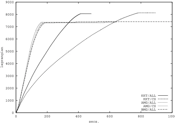
5.4 Experiments with Pattern Selection
Experiments comparing the proposed pattern selection approaches versus the Crammer and Singer one has been conducted using a dataset consisting of 10705 digits randomly taken from the NIST-3 dataset. The training set consisted of 5000 randomly chosen digits.
The optimization algorithm has been chosen among: i) The base-line Crammer and Singer orig-inal fixed-point procedure (here denoted CS); ii) AllPairsOptimizeOnPatterns (here denoted ALL); iii) BasicOptimizeOnPatterns (here denoted BAS). In the first experiments we used a cache for the kernel matrix of size 3000 that was able to contain all the matrix rows associated to the support vectors. For all the following experiments a AMD K6-II, 300MHz, with 64MB of memory has been used.
0 1000 2000 3000 4000 5000 6000 7000 8000 9000
0 200 400 600 800 1000
lagrangian
secs.
KKT/ALL KKT/CS AMG/ALL AMG/CS BMG/ALL
Figure 7: The effect of the logarithmic cooling scheme on different selection/optimization strate-gies.
0 1000 2000 3000 4000 5000 6000 7000 8000 9000
0 200 400 600 800 1000
lagrangian
secs.
0.1 Max 0.5 Max Mean
Figure 8: Comparison of different heuristics for the computation of the valueθV for the SMO-like
algorithm.
0 1000 2000 3000 4000 5000 6000 7000 8000 9000
0 500 1000 1500 2000
lagrangian
secs.
KKT/ALL AMG/ALL BMG/ALL BMG/BAS
Figure 9: Comparison of different selection strategies using the heuristic MEAN.
logarithmic function is very slow to converge to zero, and because of that, the value returned by the strategies will be soon below the threshold. In particular the logarithmic function remains on a value of about 0.1 for many iterations. While this value is pretty good for the accuracy of the KKT solution, it is not sufficient for our selection schemes. In Figure 8 different heuristics for the computation of the valueθV of the selection strategy of the SMO-like algorithm are compared.
0 1000 2000 3000 4000 5000 6000 7000 8000
0 500 1000 1500 2000
lagrangian
secs.
AMG/ALL Cache 100 BMG/ALL Cache 100 KKT/ALL Cache 100 BMG/BAS Cache 100
(a)
0 5 10 15 20 25 30 35 40 45 50
0 1000 2000 3000 4000 5000 6000
test error
secs.
KKT/ALL Cache 100 AMG/ALL Cache 100
(b)
Figure 10: The effect of the cache limitation: (a) Lagrangian value versus time; (b) test perfor-mance versus time.
are compared. In this case, the new strategies slightly outperform the one based on Crammer and Singer’s KKT conditions. Actually, as we will see in the following, this slight improvement is due to the big size of the cache of kernel matrix rows that prevents the algorithm suffering of the large amount of time spent in the computation of kernels that are not present in the cache.
same figure we can see also a quite poor performance when the basic version of the SMO-like is used as a global optimization method. This demonstrates how important is to solve the overall problem one pattern at time. In fact, this leads to a decrease of the total number of patterns selected for optimization and consequently to a decrease of the number of kernel computations. This puts also in evidence the amount of time spent in kernel computation versus the amount of time spent in the optimization. Figure 10-b clearly shows that the same argument can be applied to the recognition accuracy.
5.5 Brief Discussion
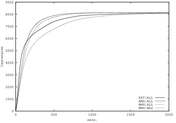
The type of strategies we have analyzed in earlier sections are very similar to the ones used by SMO (Platt, 1998), modified SMO (Keerthi et al., 1999) and svmlight (Joachims, 1999) algorithms for binary SVM. In these cases, linear constraints involving dual variables which are related to different patterns (derived by KKT conditions over the bias term) are present. However, in our case, as in the Crammer and Singer’s algorithm (Crammer and Singer, 2001), constraints involve dual variables which are related to the same pattern (but over different prototypes). This makes a difference in the analysis since it turns out that it is convenient to optimize as much as possible the reduced problem obtained for a single pattern as this optimization does not require the computation of new kernels. This claim is supported by our experimental results comparing BMG-ALL vs. BMG-BAS in Figure 10.
Also, we have shown experimentally that the use of heuristics based on the increase of the Lagrangian tend to be faster than KKT based ones, when used for pattern selection (compare BMG-ALL vs. KKT-BMG-ALL in Figure 10). This can be due to the fact that the number of different patterns selected along the overall optimization process tends to be smaller and this largely compensates the inefficiency derived by the computation of the increase of the Lagrangian and the thresholds. On the other hand, according to the same experimental analysis, KKT conditions help when used for the choice of pairs to optimize in the reduced problems obtained for a given pattern. According to these considerations, this mixed approach has been adopted in the experiments that follow.
6. Optimization of General MProtSVM
By now, we have analyzed the (static) problem obtained when the assignment is given. In this sec-tion, we describe methods for the optimization with respect to the assignmentsπas well. Naturally, the full problem is no longer convex. So, we first present an efficient procedure that guarantees to reach a stationary point of the objective function of the problem in Eq. (8) associated to MProtSVM. Then, we insert it in a stochastic search framework with the aim to improve the quality of the solu-tions we find.
6.1 Greedy Optimization of MProtSVM
Let suppose to start by fixing an initial assignment π(1) for the patterns. As we have already seen, the associated problem is then convex and can be efficiently solved for example by using the general scheme in Figure 3. Once that the optimal value for the primal, let say Pπ∗(1), has been reached, we can easily observe that the solution can be further improved by updating the assignments in such a way to associate each pattern xito a positive prototype having associated the
minimal slack value, i.e. by setting the vectorπi(2) so to have the unique 1 corresponding to the
best performing positive prototype. However, with this new assignmentπ(2), the variablesαmay no longer fulfill the second admissibility condition in Eq. (10). If this is the case, it simply means that the current solution M(α)is not optimal for the primal (although still admissible). Furthermore, α cannot be optimal for the dual given the new assignment since it not even admissible. Thus, a Lagrangian optimization, done by keeping the constraints dictated by the admissibility conditions in Eq. (10) satisfied for the new assignment, is guaranteed to obtain a newαwith a better optimal primal value Pπ∗(2), i.e. Pπ∗(2)≤Pπ∗(1). For the optimization algorithm to succeed, however, KKT conditions onα have to be restored in order to return back to a feasible solution and then finally resuming the Lagrangian optimization with the new assignment π(2). Admissibility conditions can be simply restored by settingαi =0 whenever there exists any r∈
P
i such that the conditionαr
i >0∧πri =0 holds. Note that, when the values assigned to the slack variables allow to define
a new assignment forπcorresponding to a new problem with a better optimal primal value, then, because of convexity, the Lagrangian of the corresponding dual problem will have an optimal value that is strictly smaller than the optimal dual value of the previous problem.
Performing the same procedure over different assignments, each one obtained from the previous one by the procedure described above, implies the convergence of the algorithm to a fixed-point consisting of a stationary point for the primal problem when no improvements are possible and the KKT complementarity conditions are all fulfilled by the current solution.
One problem with this procedure is that it can result onerous when dealing with large datasets or when using many prototypes since, in this case, many complete Lagrangian optimizations have to be performed. For this, we can observe that for the procedure to work, at each step, it is sufficient to stop the optimization of the Lagrangian when we find a value for the primal which is better than the last found value and this is going to happen for sure since the last solution was found not optimal. This requires only a periodic check of the primal value when optimizing the Lagrangian.
6.2 Stochastic Modifications for MProtSVM Optimization
Another problem with the procedure given in the previous section is that it leads to a stationary point (either a local minima or a saddle point) that can be very far from the best possible solution. Moreover, it is quite easy to observe that the problem we are solving is combinatorial. In fact, since the induced problem is convex for each possible assignment, then there will exist a unique optimal primal value P∗(π,α∗(π)) associated with optimal solutionsα∗(π)for the assignmentsπ. Thus, the overall problem can be reduced to find the best among all possible assignments. However, when assuming an equal number q of prototype vectors for each class, there are qnpossible solutions with many trivial symmetries.
building a sequence of solutions by first perturbing the current solution and then applying local search to that modified solution.
In the previous section, a way to perform approximated local search has been given. Let us now consider how to perturb a given solution. We propose to perform a perturbation that is variable with time and is gradually cooled by a simulated annealing like procedure.
For this, let us view the value of the primal as an energy function
E(π) =1 2||M||
2+C
∑
i
hπi,ξii.
Let suppose to have a pattern xi having slack variablesξri, r∈
P
i, and suppose that the probabilityfor the assignment to be in the state of nature s (i.e. with the s-th component set to 1) follows the law
pi(s)∝e−∆Es/T
where T is the temperature of the system and∆Es=C(ξsi−ξ yi
i )the variation of the system energy
when the pattern xi is assigned to the s-th prototype. By multiplying every term pi(s)by the
nor-malization term eC(ξyii −ξ0i)/T whereξ0
i =minr∈Piξ
r
i and considering that probabilities over alternative
states must sum to one, i.e.∑r∈Pipi(r) =1, we obtain
pi(s) =
1 Zi
e−
C(ξs i−ξ0i)
T (17)
with Zi=∑r∈Pie−
C(ξr
i−ξ0i)/T the partition function.
Thus, when perturbing the assignment for a pattern xi, each positive prototype s will be selected
with probability pi(s). From Eq. (17) it clearly appears that, when the temperature of the system is
low, the probability for a pattern to be assigned to a prototype different from the one having minimal slack value tends to 0 and we obtain a behavior similar to the deterministic version of the algorithm. The simulated annealing is typically implemented by decreasing the temperature, as the number of iterations increases, by a monotonic decreasing function T =T(t,T0).
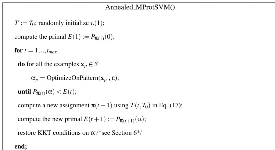
Summarizing, an efficient realization of the ILS-based algorithm is obtained by substituting the true local optimization with one step of the algorithm in Section 6.1 and is given in Figure 11.
7. Generalization Ability of MProtSVM
In this section, we give a theoretical analysis of the generalization ability of the MProtSVM model. For simplicity, we consider MProtSVM with a fixed number q of prototypes per class. We first assume training data being separated by a MProtSVM model and we give a margin based upper bound on the error that holds with high probability on a independently generated set of examples. Then, we give a growth-function based bound on the error which do not assume linear separability of training data.
Margin based generalization bound Let us suppose that an i.i.d. sample
S
of n examples and a model M are given such that the condition in Eq. (7) holds for every example inS
, i.e.∀(xi,ci)∈
S
,∃r∈P
i: hMr,xii ≥θi+1 andθi=max r∈NiAnnealed MProtSVM()
T :=T0; randomly initializeπ(1);
compute the primal E(1):=Pπ(1)(0); for t=1, ..,tmax
do for all the examples xp∈S
αp=OptimizeOnPattern(xp,ε);
until Pπ(t)(α)<E(t);
compute a new assignmentπ(t+1)using T(t,T0)in Eq. (17); compute the new primal E(t+1):=Pπ(t+1)(α);
restore KKT conditions onα/*see Section 6*/
end;
Figure 11: Fast annealed algorithm for the optimization of MProtSVM.
With this assumption, fixing a pattern xp, there will be at least one slack variableξrp, associated
with it, equal to zero. In fact, the conditionξrp=0 is true at least in the case r=yp, where ypis the
positive prototype associated to the pattern xp, i.e. such thatπ yp
p >0.
To give the margin-based bound on the generalization error, we use the same technique as in an(Platt et al., 2000) for general Perceptron DDAG1(and thus SVM-DAG also), i.e. we show how the original multiclass problem can be reduced into one made of multiple binary decisions. The structure of our proof resembles the one given in (Crammer and Singer, 2000) for single-prototype multiclass SVM.
A Perceptron DDAG is a rooted binary DAG with N leaves labelled by the classes where each of the K=m(m−1)internal nodes is associated with a perceptron able to discriminate between two classes. The nodes are arranged in a triangle with the single root node at the top, two nodes in the second layer and so on until the final layer of m leaves. The i-th node in layer j<m is connected to the i-th and(i+1)-st node in the(j+1)-st layer. A Perceptron DDAG based classification can also be though of as operating on a list of classes with associated a set of perceptrons, one for each different pair of classes in the list. The evaluation of new patterns is made by evaluating the pattern with the perceptron discriminating the classes in the first and in the last position of the list. The losing class between the two is eliminated from the list. This process is repeated until only one class remains in the list and this class is returned.
Similarly, MProtSVM classification can be thought of as operating on a list. Suppose the index of prototypes r∈R={1, . . . ,mq}are ordered according to their class
C
(r)∈ {1, . . . ,m}. Then,given a new pattern, we compare the scores obtained by the two prototypes in the head and in the tail of the list and the loser is removed from the list. This is done until only prototypes of the same class remain on the list and this is the class returned for the pattern under consideration. It is easy to show that this procedure is equivalent to the rule in Eq. (2).
In the following, we will refer to the following theorem giving a bound on the generalization error of a Perceptron DDAG:
Theorem 2 (Platt et al., 2000) Suppose we are able to classify a random sample of labelled exam-ples using a Perceptron DDAG on m classes containing K decision nodes with marginγiat node i,
then we can bound the generalization error with probability greater than 1−δto be less than
1 n(130R
2D0log(4en)log(4n) +log(2(2n)K δ ))
where D0=∑Ki=1γ−i 2, and R is the radius of a ball containing the support of the distribution. Note that, in this theorem, the marginγifor a perceptron(wi,bi)associated to the pair of classes
(r,s) is computed as γi =mincp∈{r,s}|hwi,xpi −bi|. Moreover, we can observe that the theorem
depends only on the number of nodes (number of binary decisions) and does not depend on the particular architecture of the DAG.
Going back to MProtSVM, for the following analysis we define the hyperplane wrs=Mr−Ms
for each pair of prototypes indexes r,s such that
C
(r)<C
(s). and the support of the hyperplane wrsas the subset of patterns
Γrs={i∈ {1, . . . ,n}:(r∈
P
i∧πir>0)∨(s∈P
i∧πsi >0)}.Now, we can define the margin of the classifier hrs(x) =hwrs,xias the minimum of the
(geo-metrical) margins of the patterns associated to it, i.e.
γrs=min i∈Γrs
|hrs(xi)|
||wrs||
(18)
Note that, from the hypothesis of separation of the examples and from the way we defined the margin, we have|hrs(xi)| ≥1 and hence the lower bound on the marginγrs≥ ||wrs||−1.
Now, we can show that the maximization of these margins leads to a small generalization error by demonstrating the following result.
Lemma 3 Suppose we are able to classify a random sample of labelled examples using a MProtSVM with q prototypes for each of the m classes with marginγrs when
C
(r)<C
(s), then we can boundthe generalization error with probability greater than 1−δto be less than
1 n(130R
2D log(4en)log(4n) +log(2(2n)K δ ))
Proof. First of all, we show that an MProtSVM can be reduced to a Perceptron DDAG. Let be given prototype indices r∈R={1, . . . ,mq}ordered according to their class
C
(r)∈ {1, . . . ,m}. Consider two cursors r and s initially set to the first and the last prototype in R, respectively. Now, we build a DAG node for(r,s)based on the classifier hrs. Then, recursively, left and right edges arebuilt associated to nodes(r,s−1)and(r+1,s)respectively. This is made until the condition
C
(r) =C
(s) =t holds. When this is the case, a leaf node is built instead with label t. This construction is based on the fact that there is not need to compare the scores obtained by prototypes associated to the same class.We show now that the number of nodes in the skeleton of a DAG D which is built in this way is exactly K=1
2q2m(m−1). In fact, consider the DAG D0obtained by keeping on constructing DAG nodes(r,s) until the condition r=s holds, instead of just
C
(r) =C
(s). This graph would be the same that would have been obtained by considering mq classes with one prototype each. Note that D0is balanced and it consists of 12mq(mq−1)nodes. It follows that, to obtain the DAG D, for each class y, we subtract the subDAG constructed by considering all possible ky =q(q−1)/2 pairs ofprototypes associated to that class.
Summarizing, the number of nodes of the DAG D is the number of nodes of the balanced DAG D0minus the total number of mkysubDAG nodes. That is we get:
K=1
2mq(mq−1)−m( 1
2q(q−1)) = 1 2q
2m(m
−1).
Now, we can apply Theorem 2, by considering a Perceptron DDAG with K nodes associated to pairs r,s :
C
(r)<C
(s)and the margin for the node(r,s)defined as in Eq. (18).By now, we have demonstrated that the minimization of the term D=∑r,s:C(r)<C(s)γ−2
rs
propor-tional to the margin of the nodes of the Perceptron DDAG we have constructed, leads to a small generalization error. This result can then be improved by showing how these margins are linked to the norm of the MProtSVM matrix M and finally proving the following theorem.
Theorem 4 Suppose we are able to classify a random sample of n labelled examples using a MProtSVM with q prototypes for each of the m classes and matrix M, then we can bound the gener-alization error with probability greater than 1−δto be less than
1 n
130R2q(m−1+q)||M||2log(4en)log(4n) +log(2(2n)
K
δ )
where K=1
2q2m(m−1)and R is the radius of a ball containing the support of the distribution. Proof. First of all, note that we haveγ−rs2≤ ||wrs||2=||Mr−Ms||2 and∑rMr=0.The second
condition can be easily verified. In fact, from conditions in Eq. (10), it follows
∑
r
Mr=
∑
r
∑
iyriαrixi=
∑
i(
∑
r
yriαri
| {z }
0
)xi=0.
Now, we have