Variance Reduction Techniques for Gradient Estimates in Reinforcement Learning

Variance Reduction Techniques for Gradient Estimates in

Reinforcement Learning

Evan Greensmith [email protected]

Research School of Information Sciences and Engineering Australian National University

Canberra 0200, Australia

Peter L. Bartlett [email protected]

Computer Science Division & Department of Statistics UC Berkeley

Berkeley, CA 94720, USA

Jonathan Baxter [email protected]

Panscient Pty. Ltd. 10 Gawler Terrace

Walkerville, SA 5081, Australia

Editor: Michael Littman

Abstract

Policy gradient methods for reinforcement learning avoid some of the undesirable properties of the value function approaches, such as policy degradation (Baxter and Bartlett, 2001). However, the variance of the performance gradient estimates obtained from the simulation is sometimes ex-cessive. In this paper, we consider variance reduction methods that were developed for Monte Carlo estimates of integrals. We study two commonly used policy gradient techniques, the baseline and actor-critic methods, from this perspective. Both can be interpreted as additive control variate variance reduction methods. We consider the expected average reward performance measure, and we focus on the GPOMDP algorithm for estimating performance gradients in partially observable Markov decision processes controlled by stochastic reactive policies. We give bounds for the esti-mation error of the gradient estimates for both baseline and actor-critic algorithms, in terms of the sample size and mixing properties of the controlled system. For the baseline technique, we compute the optimal baseline, and show that the popular approach of using the average reward to define the baseline can be suboptimal. For actor-critic algorithms, we show that using the true value function as the critic can be suboptimal. We also discuss algorithms for estimating the optimal baseline and approximate value function.

Keywords: reinforcement learning, policy gradient, baseline, actor-critic, GPOMDP

1. Introduction

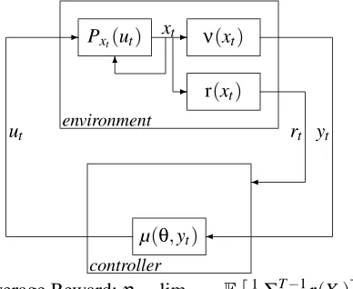
The controller can use the observations to determine which action to produce, thereby altering the POMDP state. The expectation of the average reward over possible future sequences of states given a particular controller (the expected average reward) can be used as a measure of how well a controller performs. This performance measure can then be used to select a controller that will perform well.

Given a parameterized space of controllers, one method to select a controller is by gradient ascent (see, for example, Glynn, 1990; Glynn and L‘Ecuyer, 1995; Reiman and Weiss, 1989; Ru-binstein, 1991; Williams, 1992). An initial controller is selected, then the gradient direction in the controller space of the expected average reward is calculated. The gradient information can then be used to find the locally optimal controller for the problem. The benefit of using a gradient approach, as opposed to directly comparing the expected average reward at different points, is that it can be less susceptible to error in the presence of noise. The noise arises from the fact that we estimate, rather than calculate, properties of the controlled POMDP.

Determining the gradient requires the calculation of an integral. We can produce an estimate of this integral through Monte Carlo techniques. This changes the integration problem into one of calculating a weighted average of samples. It turns out that these samples can be generated purely by watching the controller act in the environment (see Section 3.3). However, this estimation tends to have a high variance associated with it, which means a large number of steps is needed to obtain a good estimate.

GPOMDP (Baxter and Bartlett, 2001) is an algorithm for generating an estimate of the gradient in this way. Compared with other approaches (such as the algorithms described in Glynn, 1990; Rubinstein, 1991; Williams, 1992, for example), it is especially suitable for systems with large state spaces, when the time between visits to a recurrent state is large but the mixing time of the controlled POMDP is short. However, it can suffer from the problem of high variance in its estimates. We seek to alter GPOMDP so that the estimation variance is reduced, and thereby reduce the number of steps required to train a controller.

One generic approach to reducing the variance of Monte Carlo estimates of integrals is to use an additive control variate (see, for example, Hammersley and Handscomb, 1965; Fishman, 1996; Evans and Swartz, 2000). Suppose we wish to estimate the integral of the function f :

X

_→R, and we happen to know the value of the integral of another function on the same spaceϕ:

X

→R. As we have

Z

X f(x) =

Z

X

(f(x)₋ϕ(x)) + Z

Xϕ

(x) (1)

the integral of f(x)₋ϕ(x)can be estimated instead. Obviously ifϕ(x) =f(x)then we have managed to reduce our variance to zero. More generally,

Var(f₋ϕ) =Var(f)₋2Cov(f,ϕ) +Var(ϕ).

does not depend on the state, has been commonly suggested (Sutton and Barto, 1998; Williams, 1992; Kimura et al., 1995, 1997; Kimura and Kobayashi, 1998b; Marbach and Tsitsiklis, 2001). The expectation over all states of the discounted value of the state has been proposed, and widely used, as a constant baseline, by replacing the reward at each step by the difference between the reward and the average reward. We give bounds on the estimation variance that show that, perhaps surprisingly, this may not be the best choice. Our results are consistent with the experimental observations of Dayan (1990).

The second application of the control variate approach is the use of a value function. The discounted value function is usually not known, and needs to be estimated. Using some fixed, or learnt, value function in place of this estimate can reduce the overall estimation variance. Such actor-critic methods have been investigated extensively (Barto et al., 1983; Kimura and Kobayashi, 1998a; Baird, 1999; Sutton et al., 2000; Konda and Tsitsiklis, 2000, 2003). Generally the idea is to minimize some notion of distance between the value function and the true discounted value function, using, for example, TD (Sutton, 1988) or Least-Squares TD (Bradtke and Barto, 1996). In this paper we show that this may not be the best approach: selecting a value function to be equal to the true discounted value function is not always the best choice. Even more surprisingly, we give examples for which the use of a value function that is different from the true discounted value function reduces the variance to zero, for no increase in bias. We consider a value function to be forming part of a control variate, and find a corresponding bound on the expected squared error (that is, including the estimation variance) of the gradient estimate produced in this way.

While the main contribution of this paper is in understanding a variety of ideas in gradient estimation as variance reduction techniques, our results suggest a number of algorithms that could be used to augment the GPOMDP algorithm. We present new algorithms to learn the optimum baseline, and to learn a value function that minimizes the bound on the expected squared error of a gradient estimate, and we describe the results of preliminary experiments, which show that these algorithms give performance improvements.

2. Overview of Paper

Section 3 gives some background information. The POMDP setting and controller are defined, and the measure of performance and its gradient are described. Monte Carlo estimation of integrals, and how these integrals can be estimated, is covered, followed by a discussion of the GPOMDP algorithm, and how it relates to the Monte Carlo estimations. Finally, we outline the control variates that we use.

The samples used in the Monte Carlo estimations are taken from a single sequence of observa-tions. Little can be said about the correlations between these samples. However, Section 4 shows that we can bound the effect they have on the variance in terms of the variance of the iid case (that is, when samples are generated iid according to the stationary distribution of the Markov chain).

Section 6 looks at the technique of replacing the estimate of the discounted value function with some value function, in a control variate context. It shows that using the true discounted value function may not be the best choice, and that additional gains may be made. It also gives bounds on the expected squared error introduced by a value function.

Section 7 presents an algorithm to learn the optimal baseline. It also presents an algorithm to learn a value function by minimizing an estimate of the resulting expected squared error. Section 8 describes the results of experiments investigating the performance of these algorithms.

3. Background

Here we formally define the learning setting, including the performance and its gradient. We then give an intuitive discussion of the GPOMDP algorithm, starting with its approximation to the true gradient, and how it may be estimated by Monte Carlo techniques. Finally, we introduce the two variance reduction techniques studied in this paper.

3.1 System Model

A partially observable Markov decision process (POMDP) can be modelled by a system consisting of a state space,

S

, an action space,

U, and an observation space,

Y

, all of which will be considered finite here. State transitions are governed by a set of probability transition matrices P(u), where u_∈

U, components of which will be denoted p

i j(u), where i,j∈

S

. There is also an observation

processν:

S

→

P

Y, where

P

Y is the space of probability distributions over

Y

, and a reward function r :

S

→R. Together these define the POMDP(

S

,

U

,

Y

,P,ν,r).

A policy for this POMDP is a mapping µ :

Y

∗→

P

U, where

Y

∗denotes the space of all finite sequences of observations y1, . . . ,yt ∈

Y

and

P

U is the space of probability distributions over

U. If

only the set of reactive policies µ :

Y

→

PU

is considered then the joint process of state, observation and action, denoted _{Xt,Yt,Ut}, is Markov. This paper considers reactive parameterized policies

µ(y,θ), whereθ_∈RK and y_∈

Y

. A reactive parameterized policy together with a POMDP defines a controlled POMDP(

S

,

U

,

Y

,P,ν,r,µ). See Figure 1.

yt

ut

-rt

environment

6

xt

r(xt)

Pxt(ut) ν(xt)

controller

-µ(θ,yt)

Average Reward:η=limT_→∞E

₁

T∑ T−1

t=0 r(Xt)

Given a controlled POMDP the subprocess of states, {Xt}, is also Markov. A parameterized

transition matrix P(θ), with entries pi j(θ), can be constructed, with

pi j(θ) =Ey∼ν(i)

Eu∼µ(y,θ)[pi j(u)]

=

∑

y∈Y,u∈U

νy(i)µu(y,θ)pi j(u),

whereνy(i)denotes the probability of observation y given the state i, and µu(y,θ)denotes the

proba-bility of action u given the parametersθand an observation y. The Markov chain M(θ) = (

S

,P(θ))

then describes the behavior of the process_{Xt}.

We will also be interested in the special case where the state is fully observable.

Definition 1. A controlled Markov decision process is a controlled POMDP (

S

,

U

,

Y

,P,ν,r,µ)

with

Y

=

S

andνy(i) =δyi,where

δyi=

1 y=i 0 otherwise,

and is defined by the tuple(

S

,

U

,P,r,µ).

In this case the set of reactive policies contains the optimal policy, that is, for our performance measure there is a reactive policy that will perform at least as well as any history dependent policy. Indeed, we need only consider mappings to point distributions over actions. Of course, this is not necessarily true of the parameterized class of reactive policies. In the partially observable setting the optimal policy may be history dependent; although a reactive policy may still perform well. For a study of using reactive policies for POMDPs see Singh et al. (1994); Jaakkola et al. (1995); Baird (1999). For a recent survey of POMDP techniques see Aberdeen (2002).

We operate under a number of assumptions for the controlled POMDP(

S

,

U

,

Y

,P,ν,r,µ). Note that any arbitrary vector v is considered to be a column vector, and that we write v0 to denote its transpose, a row vector. Also, the operator ∇ takes a function f(θ) to a vector of its partial derivatives, that is

∇f(θ) =

∂f

(θ)

∂θ1 , . . . , ∂f(θ)

∂θK

0

,

whereθkdenotes the kthelement ofθ.

Assumption 1. For allθ∈RK the Markov chain M(θ) = (

S

,P(θ))is irreducible and aperiodic (ergodic), and hence has a unique stationary distributionπ(θ)satisfying

π(θ)0P(θ) =π(θ)0

The terms irreducible and aperiodic are defined in Appendix A. Appendix A also contains a discussion of Assumption 1 and how both the irreducibility and aperiodicity conditions may be relaxed.

Assumption 2. There is a R<∞such that for all i∈

S

,|r(i)_{| ≤}R. Assumption 3. For all u_∈

U

, y_∈

Y

andθ_∈RKthe partial derivatives

∂µu(y,θ)

∂θk

exist and there is a B<∞such that the Euclidean norms

∇µu(y,θ)

µu(y,θ)

are uniformly bounded by B. We interpret 0/0 to be 0 here, that is, we may have µu(y,θ) =0

provided_k∇µu(y,θ)k=0.The Euclidean norm of a vector v is given by

q

∑kv2k.

Note that Assumption 3 implies that

∇p_{i j}(θ)

pi j(θ)

≤

B,

where, as in Assumption 3, we interpret 0/0 to be 0, and so we may have pi j(θ) =0 provided

k∇pi j(θ)k=0. This bound can be seen from

∇p_{i j}(θ)

=

∇

∑

y∈Y,u∈U

νy(i)µu(y,θ)pi j(u)

=

_y∈Y

∑

_,u∈U

νy(i)∇µu(y,θ)pi j(u)

≤ B

∑

y_∈Y,u_∈U

νy(i)µu(y,θ)pi j(u)

= Bpi j(θ).

A useful measure of the system’s performance is the expected average reward,

η(θ)def= lim

T→∞E

"

1 T

T−1

∑

t=0

r(Xt)

#

. (2)

From Equation (24) in Appendix A we see thatη(θ) =E[r(X)_|X_∼π(θ)],and hence is independent of the starting state. In this paper we analyze certain training algorithms that aim to select a policy such that this quantity is (locally) maximized.

It is also useful to consider the discounted value function,

J_β(i,θ)def= lim

T_→∞E

"

T−1

∑

t=0

βt_r(X t)

X0=i

#

.

Throughout the rest of the paper the dependence uponθis assumed, and dropped in the notation.

3.2 Gradient Calculation

It is shown in Baxter and Bartlett (2001) that we can calculate an approximation to the gradient of the expected average reward by

∇_βη=

∑

i,j∈S

and that the limit of∇_βηasβapproaches 1 is the true gradient∇η. Note that∇_βηis a parameterized vector in RK approximating the gradient of η, and there need not exist any function f(θ) with ∇f(θ) =∇_βη.

The gradient approximation∇_βηcan be considered as the integration over the state transition space,

∇_βη= Z

(i,j)∈S×Sπi∇pi jJβ(j)

C_{(di×d j), (3)}

whereC_{is a counting measure, that is, for a countable space}

_{C, and a set A}

_⊂

_{C, we have}

C_{(A) =} card(A)when A is finite, andC_{(A) =}∞_{otherwise. Here card(A)is the cardinality of the set A. It is} unlikely that the true value function will be known. The value function can, however, be expressed as the integral over a sample path of the chain, as Assumption 1 implies ergodicity.

∇_βη= Z

(i0,i1,...)∈S×S×...

πi0(∇pi0i1)pi1i2pi2i3. . . r(i1) +βr(i2) +β

2_r(i 3) +···

C_{(di0×. . .).} To aid in analysis, the problem will be split into an integral and a sub integral problem.

∇_βη = Z

(i,j)∈S×S

Z

(x1,...)∈S×...

πi(∇pi j)δx1jpx1x2. . .(r(x1) +···)C(dx1×. . .)C(di×d j)

= Z

(i,j)∈S×Sπi(∇pi j)

Z

(x1,...)∈S×...

δx1jpx1x2. . .(r(x1) +···)C(dx1×. . .)C(di×d j).

3.3 Monte Carlo Estimation

Integrals can be estimated through the use of Monte Carlo techniques by averaging over samples taken from a particular distribution (see Hammersley and Handscomb, 1965; Fishman, 1996; Evans and Swartz, 2000). Take a function f :

X

_→Rand a probability distributionρover the space

X

. An unbiased estimate ofR

x∈Xf(x)can be generated from samples{x0,x1, . . . ,xm₋1}taken fromρby 1

m

m−1

∑

n=0

f(xn)

ρ(xn)

.

Consider a finite ergodic Markov chain M= (

S

,P)with stationary distributionπ. Generate the Markov process_{Xt}from M starting from the stationary distribution. The integral of the function

f :

S

_→Rover the space

S

can be estimated by

1 T

T−1

∑

t=0

f(Xt)

πXt .

This can be used to estimate the integral

Z

(i,j)∈S×Sπi∇pi jJβ(j)

C_{(di×d j).}

The finite ergodic Markov chain M= (

S

,P), with stationary distributionπ, can be used to create the extended Markov process_{Xt,Xt+1}and its associated chain. Its stationary distribution has the probability mass functionρ(i,j) =πipi j, allowing the estimation of the above integral by

1 T

T−1

∑

t=0

∇pXtXt+1

pXtXt+1

Jt+1, Jt=

∞

∑

s=t

βs−t_r(X

In addition to the Monte Carlo estimation, the value function has been replaced with an unbiased estimate of the value function. In practice we would need to truncate this sum; a point discussed in the next section. Note, however, that

E "

1 T

T−1

∑

t=0

∇pXtXt+1

pXtXt+1

Jt+1

#

= 1

T

T−1

∑

t=0

E

∇

pXtXt+1

pXtXt+1

E[Jt+1|Xt+1]

= E

"

1 T

T−1

∑

t=0

∇pXtXt+1

pXtXt+1

J_β(Xt+1)

#

.

We will often be looking at estimates produced by larger Markov chains, such as that formed by the process_{Xt,Yt,Ut,Xt+1}. The discussion above also holds for functions on such chains.

3.4 GPOMDP Algorithm

The GPOMDP algorithm uses a single sample path of the Markov process_{Zt}={Xt,Yt,Ut,Xt+1} to produce an estimate of∇_βη. We denote an estimate produced by GPOMDP with T samples by ∆T.

∆Tdef=

1 T

T−1

∑

t=0

∇µ_Ut(Yt)

µUt(Yt)

Jt+1, Jtdef= T

∑

s=t

βs−t_r(X

s). (5)

This differs from the estimate given in (4), but can be obtained similarly by considering the estima-tion of∇_βηby samples from_{Zt}, and noting that

∇pi j =

∑

y∈Y,u∈U

νy(i)∇µu(y)pi j(u).

GPOMDP can be represented as the two dimensional calculation

∆T =_T1 f(Z0) J1 + f(Z1) J2 + ··· + f(ZT−1) JT

d

ef

= d

ef

=

.. .

d

ef

=

g(Z0) g(Z1) ..

. g(ZT−1)

+βg(Z1) +βg(Z2)

+β2_g(Z

2) ...

..

. +βT−2g(Z_T−1)

+βT₋1_g(Z

T−1)

where f(Zt) = (∇µUt(Yt))/µUt(Yt)and g(Zt) =r(Xt+1).

One way to understand the behavior of GPOMDP is to assume that the chains being used to calculate each Jt sample are independent. This is reasonable when the chain is rapidly mixing and

T is large compared with the mixing time, because then most pairs Jt1 and Jt2 are approximately

independent. Replacing Jt by these independent versions, J(

ind)

t , the calculation becomes

∆(ind)

T

def

= _T1 f(Z0) J₁(ind) + f(Z1) J₂(ind) + ··· + f(ZT₋1) J_T(ind)

d

ef

= d

ef

=

.. .

d

ef

=

g(Z00) g(Z10) ..

. g Z(T−1)0

+βg(Z01) +βg(Z11)

+β2_g(Z

02) ...

..

. +βT−2g Z_1(T−2)

+βT−1_{g Z} 0(T₋1)

where the truncated process{Ztn}is an independent sample path generated from the Markov chain

of the associated POMDP starting from the state Zt=Zt0.

The truncation of the discounted sum of future rewards would cause a bias from ∇_βη. By considering T to be large compared to 1/(1₋β)then this bias becomes small for a large proportion of the samples. Replacing each J_t(ind)by an untruncated version, J_t(est),shows how GPOMDP can be thought of as similar to the calculation

∆(est)

T

def

= 1

T f(Z0) J

(est)

1 + f(Z1) J2(est) + ··· + f(ZT−1) JT(est)

d

ef

= d

ef

=

.. .

d

ef

=

g(Z00) g(Z10) ..

. g Z(T−1)0

+βg(Z01) +βg(Z11) +βg Z(T−1)1

+β2_g(Z

02) +β2g(Z12) +β2g Z(T−1)2

..

. ... ...

The altered∆T sum can be written as

∆(est)

T =

1 T

T₋1

∑

t=0

∇µUt(Yt) µUt(Yt)

J_t(₊est₁). (6)

3.5 Variance Reduction

Equation (1) shows how a control variate can be used to change an estimation problem. To be of benefit the use of the control variate must lower estimation variance, and the integral of the control variate must have a known value. We look at two classes of control variate for which the value of the integral may be determined (or assumed).

The Monte Carlo estimates performed use correlated samples, making it difficult to analyze the variance gain. Given that we wish to deal with quite unrestricted environments, little is known about this sample correlation. We therefore consider the case of iid samples and show how this case gives a bound on the case using correlated samples.

The first form of control variate considered is the baseline control variate. With this, the integral shown in Equation (3) is altered by a control variate of the formπi∇pi jb(i).

Z

(i,j)∈S×Sπi∇pi jJβ(j)

C_{(di×d j) =}

Z

(i,j)∈S×Sπi∇pi j Jβ(j)−b(i)

C_{(di×d j)}

+ Z

(i,j)∈S×Sπi∇pi jb(i)

C_{(di×d j)}

The integral of the control variate term is zero, since

Z

(i,j)∈S×Sπi∇pi jb(i)

C_{(di×d j) =}

∑

i∈S

πib(i)∇

∑

j∈S

pi j

=

∑

i_∈S

πib(i)∇(1)

= 0. (7)

The second form of control variate considered is constructed from a value function, V(j), a mapping

S

→R.

Z

(i,j)∈S×Sπi∇pi jJβ

(j)C_{(di×d j) =}

Z

(i,j)∈S×Sπi∇pi j Jβ

(j)₋ J_β(j)₋V(j)

C_{(di×d j)}

+ Z

(i,j)∈S×Sπi∇pi j Jβ(j)−V(j)

C_{(di×d j)}

The integral of this control variate (the last term in the equation above) is the error associated with using a value function in place of the true discounted value function. The task is then to find a value function such that the integral of the control variate is small, and yet it still provides good variance minimization of the estimated integral.

Note that the integrals being estimated here are vector quantities. We consider the trace of the covariance matrix of these quantities, that is, the sum of the variance of the components of the vector. Given the random vector A= (A1,A2, . . . ,Ak)0, we write

Var(A) =

k

∑

m=1

Var(Am) =E

(A−E[A])0(A−E[A])

=_Eh(A−E[A])2i,

where, for a vector a, a2denotes a0a.

4. Dependent Samples

In Sections 5 and 6 we study the variance of quantities that, like∆(_Test)(Equation (6)), are formed from the sample average of a process generated by a controlled (PO)MDP. From Section 3 we know this process is Markov, is ergodic, and has a stationary distribution, and so the sample average is an estimate of the expectation of a sample drawn from the stationary distribution,π(note that, as in Section 3.3, we can also look at samples formed from an extended space, and its associated stationary distributions). In this section we investigate how the variance of the sample average relates to the variance of a sample drawn fromπ. This allows us to derive results for the variance of a sample drawn fromπand relate them to the variance of the sample average. In the iid case, that is, when the process generates a sequence of samples X0, . . . ,XT−1 drawn independently from the distributionπ, we have the relationship

Var 1 T

T₋1

∑

t=0

f(Xt)

!

= 1

TVar(f(X)),

where X is a random variable also distributed according toπ. More generally, however, correlation between the samples makes finding an exact relationship difficult. Instead we look to find a bound of the form

Var 1 T

T−1

∑

t=0

f(Xt)

!

≤h

1

TVar(f(X))

,

where h is some “well behaved” function.

Definition 2. The total variation distance between two distributions p,q on the finite set

S

is given by

dTV(p,q)def=

1

2_i

∑

_∈S|pi−qi|.

Definition 3. The mixing time of a finite ergodic Markov chain M= (

S

,P)is defined as τdef

=min

t>0 : max

i,j dTV P t i,Ptj

≤e−1

,

where Pt_idenotes the ithrow of the t-step transition matrix Pt.

The results in this section are given for a Markov chain with mixing timeτ. In later sections we will useτas a measure of the mixing time of the resultant Markov chain of states of a controlled (PO)MDP, but will look at sample averages over larger spaces. The following lemma, due to Bartlett and Baxter (2002), shows that the mixing time does not grow too fast when looking at the Markov chain on sequences of states.

Lemma 1. (Bartlett and Baxter, 2002, Lemma 4.3) If the Markov chain M= (

S

,P)has mixing time τ, then the Markov chain formed by the process_{Xt,Xt+1, . . . ,Xt+k}has mixing time ˜τ, where

˜

τ_≤τln(e(k+1)).

Note 1. For a controlled POMDP, the Markov chain formed by the process

{Xt,Xt+1, . . . ,Xt+k} has the same mixing time as the Markov chain formed by the process

{Xt,Yt,Ut,Xt+1, . . . ,Yt+k−1,Ut+k−1,Xt+k}.

We now look at showing the relationship between the covariance between two samples in a sequence and the variance of an individual sample. We show that the gain of the covariance of two samples Xt,Xt+sover the variance of an individual sample decreases exponentially in s.

Theorem 2. Let M= (

S

,P)be a finite ergodic Markov chain, and letπbe its stationary distribution. Let f be some mapping f :

S

→R. The tuple(M,f)has associated positive constantsαand L (called mixing constants(α,L)) such that, for all t_≥0,

|Cov_π(t; f)_{| ≤}Lαt_Var(f(X))

where X _∼π, and Cov_π(t; f) is the auto-covariance of the process _{f(Xs)}, i.e. Covπ(t; f) =

Eπ[(f(Xs)−Eπf(Xs)) (f(Xs+t)−Eπf(Xs+t))], where Eπ[·] denotes the expectation over the chain

with initial distributionπ. Furthermore, if M has mixing timeτ,we have:

1. for reversible M, and any f, we may choose L=2e andα=exp(₋1/τ); and

2. for any M (that is, any finite ergodic M), and any f,we may choose L=p

2_|

S

|e andα=

exp(₋1/(2τ)).

Theorem 3. Let M= (

S

,P)be a finite ergodic Markov chain, with mixing timeτ, and letπbe its stationary distribution. Let f be some mapping f :

S

→R. Let_{Xt}be a sample path generated by

M, with initial distributionπ, and let X_∼π. With(M,f)mixing constants(α,L)chosen such that α≤exp(₋1/(2τ)), there is anΩ∗≤6Lτsuch that

Var 1 T

T−1

∑

t=0

f(Xt)

!

≤Ω∗

T Var(f(X)).

Provided acceptable mixing constants can be chosen, Theorem 3 gives the same rate as in the case of independent random variables, that is, the variance decreases as O(1/T). The most that can be done to improve the bound of Theorem 3 is to reduce the constantΩ∗. It was seen, in Theorem 2, that good mixing constants can be chosen for functions on reversible Markov chains. We would like to deal with more general chains also, and the mixing constants given in Theorem 2 for functions on ergodic Markov chains lead toΩ∗increasing with the size of the state space. However, for bounded functions on ergodic Markov chains we have the following result:

Theorem 4. Let M= (

S

,P)be a finite ergodic Markov chain, and letπbe its stationary distribution. If M has mixing timeτ,then for any function f :

S

→[₋c,c]and any 0<ε<e−1,we have

Var 1 T

T−1

∑

t=0

f(Xt)

!

≤ε+

1+25τ(1+c)ε+4τln1_ε

1

TVar(f(X)),

where_{Xt}is a process generated by M with initial distribution X0∼π,and X∼π.

Here we have an additional errorε,which we may decrease at the cost of a lnε−1penalty in the constant multiplying the variance term.

Consider the following corollary of Theorem 4.

Corollary 5. Let M= (

S

,P)be a finite ergodic Markov chain, and letπbe its stationary distribu-tion. If M has mixing timeτ,then for any function f :

S

→[₋c,c], we have

Var 1 T

T−1

∑

t=0

f(Xt)

!

≤ 4τln 7(1+c) + 1

4τ

1

TVar(f(X))

−1!

1

TVar(f(X))

+ (1+8τ) 1

TVar(f(X))

where_{Xt}is a process generated by M with initial distribution X0∼π,and X∼π.

Here, again, our bound approaches zero as Var(f(X))/T_→0,but at the slightly slower rate of

O 1

TVar(f(X))ln e+

1

TVar(f(X))

−1!!

,

5. Baseline Control Variate

As stated previously, a baseline may be selected with regard given only to the estimation variance. In this section we consider how the baseline affects the variance of our gradient estimates when the samples are iid, and the discounted value function is known. We show that, when using Theorem 3 or Theorem 4 to bound covariance terms, this is reasonable, and in fact the error in analysis (that is, from not analyzing the variance of∆T with baseline directly) associated with the choice of baseline

is negligible. This statement will be made more precise later.

Section 5.2 looks at the Markov chain of states generated by the controlled POMDP and is concerned with producing a baseline b_S :

S

→Rto minimize the variance

σ2

S(bS) =Varπ

∇

pi j

pi j

J_β(j)₋b_S(i)

, (8)

where, for some f :

S

×

S

→RK,Var_π(f(i,j)) =Eπ(f(i,j)₋Eπf(i,j))2 with Eπ[·]denoting the expectation over the random variables i,j with i_∼πand j_∼Pi.Equation (8) serves as a definition

ofσ2_S(bS).The section gives the minimal value of this variance, and the minimizing baseline. Addi-tionally, the minimum variance and corresponding baseline is given for the case where the baseline is a constant, b_∈R. In both cases, we give expressions for the excess variance of a suboptimal baseline, in terms of a weighted squared distance between the baseline and the optimal one. We can thus show the difference between the variance for the optimal constant baseline and the variance obtained when b=EπJ_β(i).

Section 5.3 considers a baseline b_Y :

Y

→Rfor the GPOMDP estimates. It shows how to minimize the variance of the estimate

σ2

Y(bY) =Varπ

∇

µu(y)

µu(y)

J_β(j)₋bY(y)

, (9)

where, for some f :

S

_×

Y

_×

U

_×

S

_→RK,Varπ(f(i,y,u,j)) =Eπ(f(i,y,u,j)₋Eπf(i,y,u,j))2with, in this case,Eπ[·]denoting the expectation over the random variables i,y,u,j with i_∼π,y_∼ν(i),

u_∼µ(y),and j_∼Pi(u).Equation (9) serves as a definition ofσ2_Y(bY). The case where the state space is fully observed is shown as a consequence.

5.1 Matching Analysis and Algorithm

The analysis in following sections will look at Equation (8) and Equation (9). Here we will show that the results of that analysis can be applied to the variance of a realizable algorithm for generating ∇_βηestimates. Specifically, we compare the variance quantity of Equation (9) to a slight variation of the∆T estimate produced by GPOMDP, where the chain is run for an extra S steps. We consider

the estimate

∆(+S)

T

def

= 1

T

T₋1

∑

t=0

∇µUt(Yt) µUt(Yt)

J_t(+₊₁S), Jt(+S)

def

=

T+S

∑

s=t

βs−t_r(X

s), (10)

and are interested in improving the variance by use of a baseline, that is, by using the estimate

∆(+S)

T (bY) def

= 1

T

T−1

∑

t=0

∇µUt(Yt) µUt(Yt)

J_t(+₊₁S)₋b_Y(Yt)

We delay the main result of the section, Theorem 7, to gain an insight into the ideas behind it. In Section 3.4 we saw how GPOMDP can be thought of as similar to the estimate∆(_Test),Equation (6). Using a baseline gives us the new estimate

∆(est)

T (bY) def

= 1

T

T₋1

∑

t=0

∇µUt(Yt) µUt(Yt)

J_t(₊est₁)₋b_Y(Yt)

. (11)

The term Jt(est) in Equation (11) is an unbiased estimate of the discounted value function. The

following lemma shows that, in analysis of the baseline, we can consider the discounted value function to be known, not estimated.

Lemma 6. Let _{Xt} be a random process over the space

X

. Define arbitrary functions on the

space

X

: f :

X

→R, J :

X

→R, and a :

X

→R. For all t let Jt be a random variable such that

E[Jt|Xt =i] =J(i). Then

Var 1 T

T−1

∑

t=0

f(Xt) (Jt−a(Xt))

!

−Var 1 T

T−1

∑

t=0

f(Xt) (J(Xt)−a(Xt))

!

=E 1

T

T−1

∑

t=0

f(Xt) (Jt−J(Xt))

!2

The proof of Lemma 6 is given in Appendix C, along with the proof of Theorem 7 below. Direct application of Lemma 6 gives,

Var

∆(est)

T (bY)

= Var 1 T

T₋1

∑

t=0

∇µUt(Yt) µUt(Yt)

J_β(Xt+1)−bY(Yt)

!

+E 1

T

T−1

∑

t=0

∇µUt(Yt) µUt(Yt)

J_t(₊est₁)₋J_β(Xt+1)

!2

.

Thus, we see that we can split the variance of this estimate into two components: the first is the variance of this estimate with Jt(est)replaced by the true discounted value function; and the second

is a component independent of our choice of baseline. We can now use Theorem 3 or Corollary 5 to bound the covariance terms, leaving us to analyze Equation (9).

We can obtain the same sort of result, using the same reasoning, for the estimate we are inter-ested in studying in practice:∆(+_T S)(bY)(see Equation (12) below).

Theorem 7. Let D= (

S

,

U

,

Y

,P,ν,r,µ)be a controlled POMDP satisfying Assumptions 1, 2 and 3. Let M= (

S

,P)be the resultant Markov chain of states, and letπbe its stationary distribution; M has a mixing timeτ;_{Zt}={Xt,Yt,Ut,Xt+1}is a process generated by D, starting X0∼π. Suppose that a(_·)is a function uniformly bounded by M, and

J

(j)is the random variable∑∞_s=0βsr(Ws)where

C2=20τB2R(R+M)such that for all T,S≥1 we have

Var 1 T

T−1

∑

t=0

∇µUt(Yt) µUt(Yt)

J_t(+₊₁S)₋a(Zt)

!

≤ h

τ

ln(e(S+1))

T Varπ

∇

µu(y)

µu(y)

J_β(j)₋a(i,y,u,j)

+h τln(e(S+1))

T Eπ

∇

µu(y)

µu(y)

J

(j)₋J_β(j)

2!

+ 2C2 (1₋β)2

ln1 β+ln

C1 1₋β+

K(1₋β)2 C2

(T+S)ln(e(S+1))

T β

S_,

where h :R+→R+is continuous and increasing with h(0) =0,and is given by

h(x) =9x+4x ln

C1 1₋β+

K 4x

−1

.

By selecting S=T in Theorem 7, and applying to∆(+_T S)(b_Y)with absolutely bounded b_Y, we obtain the desired result:

Var

∆(+T)

T (bY)

≤h

τ

ln(e(T+1))

T σ

2 Y(bY)

+N(D,T) +O ln(T)βT

. (12)

Here N(D,T)is the noise term due to using an estimate in place of the discounted value function, and does not depend on the choice of baseline. The remaining term is of the order ln(T)βT_{; it is}

almost exponentially decreasing in T,and hence negligible. The function h is due to the application of Theorem 4, and consequently the discussion in Section 4 on the rate of decrease applies here, that is, a log penalty is paid. In this case, forσ2_Y(b_Y)fixed, the rate of decrease is O(ln2(T)/T).

Note that we may replace(∇µu(y))/µu(y)with(∇pi j)/pi j in Theorem 7. So if the(∇pi j)/pi j

can be calculated, then Theorem 7 also relates the analysis of Equation 8 with a realizable algorithm for generating∇_βηestimates; in this case an estimate produced by watching the Markov process of states.

5.2 Markov Chains

Here we look at baselines for ∇_βη estimates for a parameterized Markov chain and associated reward function (a Markov reward process). The Markov chain of states generated by a controlled POMDP (together with the POMDPs reward function) is an example of such a process. However, the baselines discussed in this section require knowledge of the state to use, and knowledge of

(∇pi j(θ))/pi j(θ)to estimate. More practical results for POMDPs are given in the next section.

Consider the following assumption.

Assumption 4. The parameterized Markov chain M(θ) = (

S

,P(θ))and associated reward function r :

S

→Rsatisfy: M(θ)is irreducible and aperiodic, with stationary distributionπ; there is a R<∞

For any controlled POMDP satisfying Assumptions 1, 2 and 3, Assumption 4 is satisfied for the Markov chain formed by the subprocess_{Xt}together with the reward function for the controlled

POMDP.

Now consider a control variate of the form

ϕS(i,j)def=πi∇pi jbS(i)

for estimation of the integral in Equation (3). We refer to the function bS:

S

→Ras a baseline. As shown in Section 3.5, the integral of the baseline control variateϕ_S(i,j)over

S

×

S

can be calculated analytically and is equal to zero. Thus an estimate of the integral

Z

(i,j)∈S×S πi∇pi jJβ(j)−ϕS(i,j)

C_{(di×d j)}

forms an unbiased estimate of∇_βη.

The following theorem gives the minimum variance, and the baseline to achieve the minimum variance. We useσ2_S to denote the variance of the estimate without a baseline,

σ2

S=Varπ

∇

pi j

pi j

J_β(j)

,

and we recall, from Equation (8), thatσ2_S(bS)denotes the variance with a baseline, σ2

S(bS) =Varπ

∇

pi j

pi j

J_β(j)₋bS(i)

.

Theorem 8. Let M(θ) = (

S

,P(θ))and r :

S

→Rbe a parameterized Markov chain and reward function satisfying Assumption 4. Then

σ2 S(b∗S)

def

= inf bS∈RS

σ2

S(bS) =σ2S−Ei∼π



 

E h

(∇pi j/pi j)2Jβ(j)

i

i2

E h

(∇pi j/pi j)2

i

i 



,

where E[_·|i]is the expectation over the resultant state j conditioned on being in state i, that is, j_∼Pi, andRS is the space of functions mapping

S

toR. This infimum is attained with the baseline

b∗_S(i) =E h

(∇pi j/pi j)2Jβ(j)

i

i

E h

(∇pi j/pi j)2

i

i .

The proof uses the following lemma.

Lemma 9. For any b_S,

σ2

S(bS) =σ2S+Eπ

"

b2_S(i)E "

∇

pi j

pi j

2

i

#

−2bS(i)E

"

∇

pi j

pi j

2

J_β(j)

i

##

Proof.

σ2

S(bS) = Eπ

∇

pi j

pi j

J_β(j)₋b_S(i) −Eπ

∇

pi j

pi j

J_β(j)₋b_S(i)

2

= Eπ

∇

pi j

pi j

J_β(j)₋Eπ

∇

pi j

pi j

J_β(j)

−

∇

pi j

pi j

bS(i)−Eπ

∇

pi j

pi j

bS(i)

2

= σ2 S+Eπ

"

∇

pi j

pi j

bS(i)

2

−2

∇

pi j

pi j

bS(i)

0∇

pi j

pi j

J_β(j)

#

(13)

= σ2 S+Ei∼π

"

b2_S(i)_E " ∇ p˜ı˜ p˜ı˜ 2

˜ı=i

#

−2bS(i)E

"

∇

p˜ı˜ p˜ı˜

2

J_β(˜)

˜ı=i

##

,

where Equation (13) uses

Eπ

∇

pi j

pi j

b_S(i)

= Z

(i,j)∈S×Sπi∇pi jbS(i)

C_{(di×d j) =0,}

from (7).

Proof of Theorem 8. We use Lemma 9 and minimize for each i_∈

S

. Differentiating with respect to each b_S(i)gives

2bS(i)E

"

∇

pi j

pi j

2 i #

−2E "

∇

pi j

pi j

2

J_β(j) i # = 0

⇒bS(i) =

E h

(∇pi j/pi j)2Jβ(j)

i i E h

(∇pi j/pi j)2

i

i ,

which implies the result.

The following theorem shows that the excess variance due to a suboptimal baseline function can be expressed as a weighted squared distance to the optimal baseline.

Theorem 10. Let M(θ) = (

S

,P(θ))and r :

S

→Rbe a parameterized Markov chain and reward function satisfying Assumption 4. Then

σ2

S(bS)−σ2S(b∗S) =Eπ

"

∇

pi j

pi j

2

b_S(i)₋b∗_S(i)2 #

.

Proof. For each i_∈

S

, define Siand Wias

Si = E

"

∇

pi j

pi j

2 i # ,

Wi = E

"

∇

pi j

pi j

2

Lemma 9 and the definition of b∗_S in Theorem 8 imply that

σ2

S(bS)−σ2S(b∗S) = Eπ

b2_S(i)Si−2bS(i)Wi+

W_i2 Si

= Eπ

bS(i)

p

Si−

Wi

√

Si

2

= Eπ

h

bS(i)−b∗S(i)

2

Si

i

= Eπ

"

∇

pi j

pi j

2

b_S(i)₋b∗_S(i)2 #

.

The following theorem gives the minimum variance, the baseline to achieve the minimum vari-ance, and the additional variance away from this minimum, when restricted to a constant baseline, b_∈R. We useσ2_S(b)to denote the variance with constant baseline b,

σ2

S(b) =Varπ

∇

pi j

pi j

J_β(j)₋b

. (14)

The proof uses Lemma 9 in the same way as the proof of Theorem 8. The proof of the last statement follows that of Theorem 10 by replacing Si with S=EπSi, and Wi with W=EπWi.

Theorem 11. Let M(θ) = (

S

,P(θ))and r :

S

→Rbe a parameterized Markov chain and reward function satisfying Assumption 4. Then

σ2 S(b∗)

def

= inf

b∈Rσ 2

S(b) =σ2S−

Eπ

h

(∇pi j/pi j)2Jβ(j)

i2

Eπ(∇pi j/pi j)2

.

This infimum is attained with

b∗=Eπ h

(∇pi j/pi j)2Jβ(j)

i

Eπ(∇pi j/pi j)2

.

The excess variance due to a suboptimal constant baseline b is given by,

σ2

S(b)−σ2S(b∗) =Eπ

∇

pi j

pi j

2

(b₋b∗)2.

A baseline of the form b=EπJ_β(i)is often promoted as a good choice. Theorem 11 gives us a tool to measure how far this choice is from the optimum.

Corollary 12. Let M(θ) = (

S

,P(θ))and r :

S

→Rbe a Markov chain and reward function satisfy-ing Assumption 4. Then

σ2

S(EJβ(i))−σ2S(b∗) =

Eπ(∇pi j/pi j)2EπJβ(j)−Eπ

h

(∇pi j/pi j)2Jβ(j)

i2

Eπ(∇pi j/pi j)2

Notice that the sub-optimality of the choice b=_EπJ_β(i)depends on the independence of the random variables(∇pi j/pi j)2and Jβ(j); if they are nearly independent,EπJβ(i)is a good choice.

Of course, when considering sample paths of Markov chains, Corollary 12 only shows the difference of the two bounds on the variance given by Theorem 7, but it gives an indication of the true distance. In particular, as the ratio of the mixing time to the sample path length becomes small, the difference between the variances in the dependent case approaches that of Corollary 12.

5.3 POMDPs

Consider a control variate over the extended space

S

×

Y

×

U

×

S

of the form

ϕ(i,y,u,j) =πiνy(i)∇µu(y)pi j(u)b(i,y).

Again, its integral is zero.

Z

(i,y,u,j)∈S×Y×U×Sϕ

(i,y,u,j)C_{(di×dy×du×d j)}

=

∑

i_∈S,y_∈Y

πiνy(i)b(i,y)∇

∑

u∈U,j∈S

µu(y)pi j(u)

!

=0.

Thus an unbiased estimate of the integral

Z

(i,y,u,j)∈S×Y×U×S πiνy(i)∇µu(y)pi j(u)Jβ(j)−ϕ(i,y,u,j)

C_{(di×dy×du×d j)}

is an unbiased estimate of∇_βη. Here results analogous to those achieved for ϕ_S(i,j)can be ob-tained. However, we focus on the more interesting (and practical) case of the restricted control variate

ϕY(i,y,u,j) def

=πiνy(i)∇µu(y)pi j(u)bY(y).

Here, only information that can be observed by the controller (the observations y) may be used to minimize the variance. Recall, from Equation (9), we useσ2_Y(bY)to denote the variance with such a restricted baseline control variate,

σ2

Y(bY) =Varπ

∇

µu(y)

µu(y)

J_β(j)₋b_Y(y)

.

We useσ2_Y to denote the variance without a baseline, that is σ2

Y =Varπ

∇

µu(y)

µu(y)

J_β(j)

.

We have the following theorem.

Theorem 13. Let D= (

S

,

U

,

Y

,P,ν,r,µ) be a controlled POMDP satisfying Assumptions 1, 2 and 3, with stationary distributionπ. Then

σ2 Y(b∗Y)

def

= inf bY∈RY

σ2

Y(bY) =σ2Y−Eπ



 

Eπ

h

(∇µ_u(y)/µu(y))2Jβ(j)

y

i2

Eπ

h

(∇µ_u(y)/µu(y))2

y

i 



whereEπ[·|y]is the expectation (ofπ-distributed random variables, that is, random variables dis-tributed as inEπ[_·]) conditioned on observing y, and this infimum is attained with the baseline

b∗_Y(y) =Eπ h

(∇µ_u(y)/µu(y))2Jβ(j)

y

i

Eπ

h

(∇µ_u(y)/µu(y))2

y

i .

Furthermore, when restricted to the class of constant baselines, b_∈R, the minimal variance occurs with

b∗=Eπ h

(∇µ_u(y)/µu(y))2Jβ(j)

i

Eπ(∇µ_u(y)/µu(y))2

.

We have again used b∗ to denote the optimal constant baseline. Note though that the b∗ here differs from that given in Theorem 11. The proof uses the following lemma.

Lemma 14. For any b_Y,

σ2

Y(bY) =σ2Y +Eπ

"

b2_Y(y)_Eπ "

∇

µu(y)

µu(y)

2

y

#

−2bY(y)Eπ

"

∇

µu(y)

µu(y)

2

J_β(j)

y

##

.

Proof. Following the same steps as in the proof of Lemma 9,

σ2

Y(bY) = Eπ

∇

µ_u(y)

µu(y)

J_β(j)₋b_Y(y) −Eπ

∇

µ_u(y)

µu(y)

J_β(j)₋b_Y(y)

2

= σ2_Y+Eπ

"

∇

µ_u(y)

µu(y)

b_Y(y)

2

−2

∇

µ_u(y)

µu(y)

b_Y(y)

0∇

µ_u(y)

µu(y)

J_β(j)

#

= σ2_Y+

∑

y

"

b2_Y(y)

∑

i,u,j

πiνy(i)µu(y)pi j(u)

∇

µ_u(y)

µu(y)

2!

−2b_Y(y)

∑

i,u,j

πiνy(i)µu(y)pi j(u)

∇

µ_u(y)

µu(y)

2

J_β(j) !#

.

Note that for functions a :

Y

→Rand f :

S

×

Y

×

U

×

S

→R

∑

y

a(y)

∑

˜ı,u˜,˜

π˜ıνy(˜ı)µu˜(y)p˜ı˜(u˜)f(˜ı,y,u˜,˜)

=

∑

y

a(y)

∑

i

πiνy(i)

∑

˜ı,y˜,u˜,˜

δy ˜yπ˜ıνy(˜ı)µu˜(y)p˜ı˜(u˜) ∑iπiνy(i)

f(˜ı,y˜,u˜,˜)

=

∑

i,y

πiνy(i)a(y)

∑

˜ı,y˜,u˜,˜

Pr_{˜ı,y˜,u˜,˜_|y˜=y_}f(˜ı,y˜,u˜,˜)

= Eπ[a(y)Eπ[f(i,y,u,j)_|y]],

Proof of Theorem 13. We apply Lemma 14 and minimize for each bY(y)independently, to obtain

bY(y) =

Eπ

h

(∇µu(y)/µu(y))2Jβ(j)

y

i

Eπ

h

(∇µu(y)/µu(y))2

y

i .

Substituting gives the optimal variance. A similar argument gives the optimal constant baseline.

Example 1. Consider the k-armed bandit problem (for example, see Sutton and Barto, 1998). Here each action is taken independently and the resultant state depends only on the action performed; that is µu(y) =µuand pi j(u) =pj(u).So, writing Rβ=EU0∼µ[∑t∞=1βtr(Xt)],we have

∇_βη = _Eπ

∇

µu(y)

µu(y)

J_β(j)

= Eu∼µ

∇

µu

µu

r(j) +R_β

= Eu∼µ

∇

µu

µu

r(j)

.

Note that this last line isβindependent, and it follows from lim_β→1∇βη=∇ηthat

∇η=∇_βη _∀β_∈[0,1]. (15)

For k=2 (2 actions{u1,u2}) we have µu1+µu2=1 and∇µu1=−∇µu2, and so the optimal constant

baseline is given by

b∗ = Eπ h

(∇µu(y)/µu(y))2Jβ(j)

i

Eπ(∇µu(y)/µu(y))2

= Eu∼µ h

(∇µu/µu)2r(j)

i

Eu∼µ(∇µu/µu)2

+R_β

= µu1(∇µu1/µu1)

2

E[r_|u1] +µu2(∇µu2/µu2)

2

E[r_|u2] µu1(∇µu1/µu1)

2_+µ

u2(∇µu2/µu2)

2 +Rβ

= µu1µu2

µu1+µu2

1 µu1

E[r_|u1] + 1 µu2

E[r_|u2]

+R_β

= µu2E[r|u1] +µu1E[r|u2] +Rβ,

where we have usedE[r_|u]to denoteEj∼p(u)r(j).From (15) we know thatβmay be chosen

arbi-trarily. Choosingβ=0 gives R_β=0 and we regain the result of Dayan (1990).

In the special case of a controlled MDP we obtain the result that would be expected. This follows immediately from Theorem 13.

Corollary 15. Let D= (

S

,

U

,P,r,µ)be a controlled MDP satisfying Assumptions 1, 2 and 3, with stationary distributionπ. Then

inf b_Y∈RSσ

2

Y(bY) =σ2Y−Ei∼π



 

E h

(∇µ_u(i)/µu(i))2Jβ(j)

i

i2

E h

(∇µ_u(i)/µu(i))2

i

i 



and this infimum is attained with the baseline

bY(i) =

Eh(∇µ_u(i)/µu(i))2Jβ(j)

i

i

Eh(∇µ_u(i)/µu(i))2

i

i .

The following theorem shows that, just as in the Markov chain case, the variance of an estimate with an arbitrary baseline can be expressed as the sum of the variance with the optimal baseline and a certain squared weighted distance between the baseline function and the optimal baseline function.

Theorem 16. Let(

S

,

U

,

Y

,P,ν,r,µ)be a controlled POMDP satisfying Assumptions 1, 2 and 3, with stationary distributionπ.Then

σ2

Y(bY)−σ2Y(b∗Y) =Eπ

"

∇

µu(y)

µu(y)

2

b_Y(y)₋b∗_Y(y)2 #

.

Furthermore if the estimate using b∗, the optimal constant baseline defined in Theorem 13, has varianceσ2_Y(b∗), we have that the varianceσ2_Y(b)of the gradient estimate with an arbitrary constant baseline is

σ2

Y(b)−σ2Y(b∗) =Eπ

∇

µu(y)

µu(y)

2

(b₋b∗)2.

Proof. For each y_∈

Y

, define Syand Wyas

Sy = E

"

∇

µu(y)

µu(y)

2

y

#

,

Wy = E

"

∇

µu(y)

µu(y)

2

J_β(j)

y

#

.

Follow the steps in Theorem 10, replacing Si with Sy,and Wi with Wy.The constant baseline case

follows similarly by considering S=EπSyand W=EπWy.

In Section 7.1 we will see how Theorem 16 can be used to construct a practical algorithm for finding a good baseline. In most cases it is not possible to calculate the optimal baseline, b∗_Y, a priori. However, for a parameterized class of baseline functions, a gradient descent approach could be used to find a good baseline. Section 7.1 explores this idea.

As before, Theorem 16 also gives us a tool to measure how far the baseline b=EπJ_β(i)is from the optimum.

Corollary 17. Let D= (

S

,

U

,

Y

,P,ν,r,µ) be a controlled POMDP satisfying Assumptions 1, 2 and 3, with stationary distributionπ.Then

σ2

Y(EπJβ(i))−_binf ∈Rσ

2 Y(b) =

Eπ(∇µu(y)/µu(y))2EπJβ(j)−Eπ

h

(∇µu(y)/µu(y))2Jβ(j)

i2

Eπ(∇µ_u(y)/µu(y))2

.

As in the case of a Markov reward process, the sub-optimality of the choice b=EπJ_β(i) de-pends on the independence of the random variables(∇µ_u(y)/µu(y))2and Jβ(j); if they are nearly