The Hybrid Dynamic Prototype Construction and Parameter Optimization with Genetic Algorithm for Support Vector Machine

The Hybrid Dynamic Prototype Construction and Parameter

Optimization with Genetic Algorithm for Support Vector Machine

Chun-Liang Lu

1,2,*

, I-Fang Chung

1

and Tsun-Chen Lin

3

1

Institute of Biomedical Informatics, National Yang-Ming University, Taipei, Taiwan.

2

Department of Applied Information and Multimedia, Ching Kuo Institute of Management and Health, Keelung County, Taiwan.

3

Department of Computer and Communication Engineering, Dahan Institute of Technology, Hualien County, Taiwan.

Received 06 July 2015; received in revised form 21 September 2015; accepted 28 September 2015

Abstract

The optimized hybrid artificial intelligence model is a potential tool to deal with construction engineering

and management problems. Support vector machine (SVM) has achieved excellent performance in a wide

variety of applications. Nevertheless, how to effectively reduce the training complexity for SVM is still a serious

challenge. In this paper, a novel order-independent approach for instance selection, called the dynamic

condensed nearest neighbor (DCNN) rule, is proposed to adaptively construct prototypes in the training dataset

and to reduce the redundant or noisy instances in a classification process for the SVM. Furthermore, a hybrid

model based on the genetic algorithm (GA) is proposed to simultaneously optimize the prototype construction

and the SVM kernel parameters setting to enhance the classification accuracy. Several UCI benchmark datasets

are considered to compare the proposed hybrid GA-DCNN-SVM approach with the previously published

GA-based method. The experimental results illustrate that the proposed hybrid model outperforms the existing

method and effectively improves the classification performance for the SVM.

Keywords: Genetic Algorithm (GA), Dynamic Condensed Nearest Neighbor (DCNN), Support Vector Machine

(SVM).

1. Introduction

The support vector machine (SVM) was first proposed by Vapnik [1] and has been successful as a high performance

classifier in several domains including data mining and the machine learning areas [2]. The decision boundary of SVM only

depends on a small part of training instances. Therefore, if only instances near the boundary are selected, the training of

SVM can be efficient and thus classification accuracy is kept. However, the performance of SVM is sensitive to how the

kernel parameters are set [3]. As a result, the appropriate instance selection and kernel parameters setting must perform

simultaneously to improve the SVM classifier.

In the literature, several data reduction algorithms have been proposed that extract a consistent subset of the overall

training set including Condensed Nearest Neighbor (CNN), Modified CNN (MCNN), Fast CNN (FCNN), and others [4-7].

These algorithms have been shown to achieve condensation ratios corresponding to a small percentage of the overall training

set and to obtain the comparable classification accuracy. However, these papers merely focused on data reduction without

dealing with features selection to reduce the irrelevant features for the classifier.

Feature selection algorithms may be widely categorized into two groups: the filter and the wrapper approaches [8-9].

The filter approaches select highly ranked features based on a statistical score as a preprocessing step. Wrapper approaches,

on the contrary, directly use the induction algorithm to evaluate the feature subsets. They generally outperform filter methods

in terms of classification accuracy, but are computationally more intensive. Huang and Wang [3] proposed a GA-based

feature selection method that optimized both the feature selection and parameters setting for the SVM classifier. Based on

the experimental results obtained, the authors claimed that the algorithm may work superior to the conventional grid search

algorithm. However, they did not take into account the treatment of these redundant or noisy instances in a classification

process. So far, to the best of our knowledge, there is no other research using an evolutionary algorithm to simultaneously

deal with these three type problems, including essential training instances extraction, input features selection, and SVM

parameters setting as mentioned above.

In this paper, a new data reduction algorithm named dynamic CNN (DCNN) algorithm, which differs from the original

CNN in its employments of the voting scheme, is proposed to adaptively construct prototypes with merged rate threshold.

Second, the proposed GA-DCNN-SVM model hybridized the prototype construction, feature selection and kernel parameters

optimization methods with genetic algorithm, exhibiting high efficiency in terms of classification accuracy for SVM. The

rest of this paper is organized as follows. Section 2 describes the related works including the basic SVM, the CNN rule, and

GA concepts. Section 3 details the research methodology, the prototype voting scheme, DCNN rule, and the proposed hybrid

model in this study. Section 4 contains the experimental results from several UCI benchmark datasets and comparison with

the GA-based previously published method. Finally, conclusions are given in section 5.

2. Related Works

2.1. Basic SVM Classifier

SVM starts from a linear classifier and searches the optimal hyperplane with maximal margin. The main motivating

criterion is to separate the various classes in the training set with a surface that maximizes the margin between them. It is an

approximate implementation of the structural risk minimization induction principle that aims to minimize a bound on the

generalization error of a model [2].

Given a training set of instance-label pairs (xi,yi),i1, 2,...,m where

n i

x R _and yi  { 1, 1}. The

generalized linear SVM finds an optimal separating hyperplane f x( ) w x b by solving the following optimization

problem:

, , 1

1 2

Minimize

m T

i

w b i

w w C











Subject to: ( ) 1 0

0

i i i

i

y w x b 



       

(1)

where C is a penalty parameter on the training error, and



i _{is the non-negative slack variables. This optimization model}

can be solved using the Lagrangian method, which maximizes the same dual variables Lagrangian LD() as Eq. (2) as in

Copyright © TAETI

1 , 1

1

Maximize ( )

2

m m

D i i j i j i j

i i j

L y y x x

     









  

Subject to: 0i C, i1, 2,...,m and

1 0 m i i i y



 



(2)

To solve the optimal hyperplane, a dual Lagrangian _{( )}

D

L



must be maximized with respect to non-negative

i



under the constrains

1 0 m i i i y   



and 0



iC. The penalty parameter C is a constant to be chosen by the user. A

larger value of C corresponds to assigning a higher penalty to the errors. After the optimal solution *

i



is obtained, the

optimal hyperplane parameters

w

* and

b

* can be determined. The optimal decision hyperplane * *

( , , )

f x



b can be

written as:

* * * * * *

1

( ,

,

)

m

i i i i

f x



b

y



x x

b

w

x

b







   







(3)

Linear SVM can be generalized to non-linear SVM via a mapping function



, which is also called the kernel function,

and the training data can be linearly separated by applying the linear SVM formulation. The inner product

((x_i)(x_j)) is calculated by the kernel function k x x( _i, _j) for training data. By introducing the kernel function, the non-linear SVM (optimal hyperplane) has the following forms:

* * * * * *

1 1

( , , ) ( ) ( ) ( , )

m m

i i i i i i

i i

f x



b y



x x b y



k x x b

 





     



 (4)

Though new kernel functions are being proposed by researchers, there are four basic kernels as follows:

Linear: _{( , )} T

i j i j

k x x x x (5)

Polynomial: k x x( ,i j)(



x xiT jr) ,d



0 (6)

Radial Basis Function: 2

( ,i j) exp( || i j || ), 0

k x x  



x x



 (7)

Sigmoid: _{( , ) tanh(} T ₎

i j i j

k x x  x x r (8)

Radial basis function (RBF) is a common kernel function as Eq. (7). In order to improve SVM, the kernel parameter in

the kernel function should be set appropriately.

2.2. The Condensed Nearest Neighbor (CNN) Algorithm

The nearest neighbor (NN) rule [10-11] assigns an unclassified sample to the same class as the nearest of the N stored

labeled samples of the training set. The rule is simple, and with an unlimited number of instances, the risk in making an NN

decision is never worse than twice the Bayes risk [12]. But, as all the labeled samples of the training set must be searched to

classify a test sample, the NN method imposes large storage and computational requirements. In order to reduce the both

storage space and computational time requirements, the Condensed Nearest Neighbor (CNN) rule first introduced by Hart [4]

is that patterns in the training set may be very similar and some do not add extra information and thus may be discarded. In

the CNN rule, prototype-subset ones aim to select a subset of the training set that classifies the remaining data correctly through the NN rule. Using a prototype subset, instead of the entire training set, to implement the NN rule has the additional

advantage that it may guarantee better classification accuracy [6]. The concept of the CNN algorithm can be formalized as

The CNN algorithm uses two bins, called training set S with c-class and prototype subset P. Initially, randomly select one sample from S to P for each class c. Then, we pass one by one over the samples in S per epoch and classify each pattern

x

_i



S

using P as the prototype set. During the scan, whenever a pattern

x

_iis misclassified, it is transferred from S to

P and the prototype subset is augmented; otherwise the pattern

x

_iis called merged into P and still left in S. The algorithm terminates when no pattern is transferred during a complete pass of S and no new prototype is added to P. The procedure can

be formalized as follows.

Step 1: The first sample is randomly selected and copied from S to P for each class c.

Step 2: Check each pattern

x

_i



S

using P as the prototype subset. If all patterns have been merged into P, terminate the process; otherwise, go to Step 3.

Step 3: For each class c, if there are any unmerged samples, randomly select one and add the pattern to P; otherwise, no new

prototype is added to class c. Go to Step 2.

2.3. Genetic Algorithm

Genetic Algorithm (GA) is one of the most effective approaches for solving optimization problem. The basic principles

of GA were first proposed by Holland [13] for the formal examination of the mechanisms of natural adaptation, since then,

the algorithm has been modified to solve computational problems in research.

The GA is a stochastic search method based on the mechanics of natural selection and the process of evolution. An

implementation of a GA begins with a population of random chromosomes which can be represented by binary strings. The

members of the population are usually strings which encode a candidate solution to the problem to be solved. Members of

the population at each generation are evaluated, and chromosomes are selected for reproduction by calculating the fitness

value. The better chromosomes have higher probability to be selected into the recombination pool using the roulette wheel or

other tournament selection methods. After selection and reproduction operation, new population is generated by perturbing

the current solutions via crossover and mutation. Crossover takes two individuals called parents and produces two new

individuals called the offspring by swapping parts of the parents. This operator allows information exchange between

candidate solutions and new solution regions in the search space to be explored. Mutation serves to prevent premature loss of

population diversity by randomly sampling new points in the search space. The evolutionary process executes many

generations until the termination condition is met or by finding an acceptable solution by some criterion.

3. Methods

The original CNN has been used to iteratively select some samples and ignores others that can be absorbed for data

reduction algorithm. In this section, we extend this concept to propose the dynamic CNN approach, which differs from the

CNN rule in its employment of a strong absorption criterion, to achieve consistency efficiently for classification problems.

Some preliminary definitions are described as follows. Assume that we are given a dataset in which



( i, i), 1, 2,...,



S  x y i m is a set of m number of samples with well-defined class labels. ( 1, 2,..., )

T

i i i iD

x  x x x is

the vector of dataset for the i-th sample describing in D-dimensional Euclidean space and yiL{c c1, 2,...,cq} is the

class label associated with xi, where q is the number of classes. The distance between any two vectors xi and xj using

Copyright © TAETI

1/ 2 2 1 ( , ) ( ) D

i j i j ik jk

k

d x x x x x x



 

  _  _





 (9)

3.1. The Prototype Voting Scheme (PVS) scheme

Majority vote is one of the simplest and intuitive ensemble combination techniques. Consider the n samples, c-class dataset U from S, given an instance

x

_iof U, the Nearest Neighbors’ Distance Vector (NNDV) of

x

_iaccording to a distance d

is:

,1, ,2, , , , 1, , ,

( )i i c i c i j c i n c i n c ,

NNDV x  d d d d  d  (10)

, ,

1, ( , ) min ( , )

0, ( , ) min ( , )

1, 2,..., , 1, 2,..., , {1, 2,..., }.

i j j i j

i j c

i j j i j

d x x d x x and i j

d

d x x d x x or i j

i n j n c q

     _{ }     (11)

We pass one by one over all of the instances in U, the outputs of NNDV in U are first organized into a Decision Prototype Matrix (DPM) as shown in Fig. 1. The column for d_{1, ,j c} to

, ,

n j c

d represents the support from samples

x

₁ to

n

x for the candidate point

x

j, and the row di,1,c to di n c, , is the NNDV of xi. The vote will then result in an ensemble decision for the candidate point

x

, and the



value is:

, , 1 1 arg max n n

i j c j

i

d 

 _





(12)

1,2, 1, , 1, 1, 1, ,

2,1, 2, , 2, 1, 2, ,

,1, ,2, , , , 1, , ,

1,1, 1,2, 1, , 1, ,

,1, ,2, , , , 1,

0

0

0

0

c j c n c n c

c j c n c n c

i c i c i j c i n c i n c

n c n c n j c n n c

n c n c n j c n n c

d d d d

d d d d

d d d d d

DPM

d d d d

d d d d

                              

Fig. 1 Decision Prototype Matrix for the PVS scheme

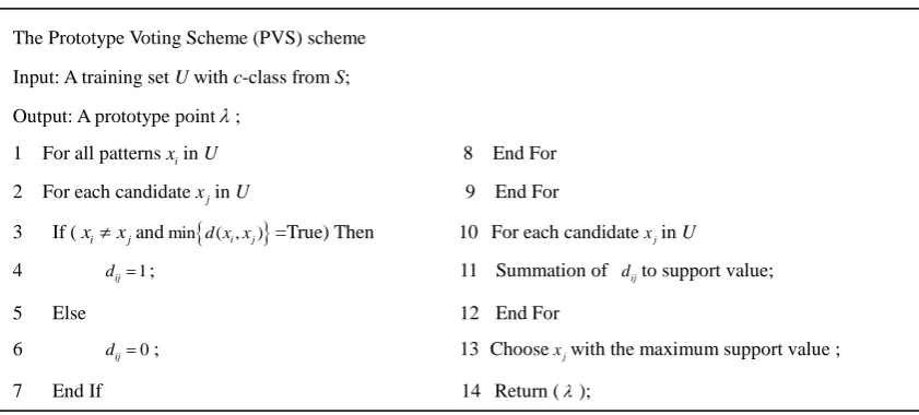
The candidate point with the highest total support is then chosen as the prototype. The pseudo code of the proposed

Prototype Voting Scheme (PVS) algorithm is shown in Fig. 2. The CNN rule is randomly to select candidate point for the

prototype construction process. The PVS algorithm differs from CNN, is order-independent and always returns the same

consistent prototype subset from the original sample set.

Fig. 2 Pseudo code of the PVS scheme

The Prototype Voting Scheme (PVS) scheme

Input: A training set U with c-class from S;

Output: A prototype point;

1 For all patternsx_iin U 8 End For

2 For each candidatexjin U 9 End For

3 If (x_ix_jandmin



d x x( ,i j)



=True) Then 10 For each candidatexjin U

4 dij1; 11 Summation of dijto support value;

5 Else 12 End For

6 dij0; 13 Choosexjwith the maximum support value ;

3.2. The Dynamic Condensed Nearest Neighbor (DCNN) rule

As the CNN rule randomly chooses samples as prototypes and checks whether all samples have been fully merged into

prototype subset, the PVS algorithm is used to improve the randomly select process in Prototype Construction stage and the

adaptively merged rate coefficient



_m for dynamically tuning the flexible criterion in Merge Detection process. Hence, it is called the Dynamic CNN (DCNN) algorithm.

The DCNN rule has the following advantages. First, it incorporates simply voting scheme in prototype construction

process to always return the same consistent training subset independent of the order in which the data is processed and can

thus outperform the CNN rule. Second, the employment of the adaptively merged rate coefficient in the Merge Detection

process is flexible to edit out noisy instances, to reduce the superfluous instances and makes the machine less sensitive to

noises and outliners. The adaptively merged rate coefficient, denoted as _[0,1]

m

  , is defined as the ratio of the number of

instances merged into prototypes to the number of overall dataset and evaluated by Eq. (13). The number of instances

merged into prototypes and the number of overall dataset are indicated by

merge

N and N_total, respectively.

merge _100% m

total

N N

   (13)

The proposed DCNN algorithm is described as follows.

Step 1: Prototype Initiation: For each class c, adopts the PVS algorithm to select a c-sample as a new c-prototype.

Step 2: Merge Detection: Detect whether all samples have been achieved the user defined merged rate threshold



_m. If so,

terminate the process; otherwise, proceed to the Step 3.

Step 3: Prototype Augmentation: For each c, if there are any un-merged c-samples, applies the PVS algorithm to construct a

new c-prototype; otherwise, no new prototype is added to class c. Proceed to Step 2.

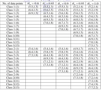
Table 1 The numerical values of the prototype data points with five values of merged rate

No. of data points m 0.8 m0.85 m0.9 m0.95 m 1.0

Class 1 (1) (5.5,1.3) (5.5,1.3) (5.5,1.3) (5.2,1.4) (5.2,1.4) Class 1 (2) (6.4,1.5) (5.6,1.5) (5.6,1.5) (5.5,1.3) (5.2,1.9) Class 1 (3) (6.9,1.5) (6.3,1.6) (5.6,1.8) (5.6,1.5) (5.5,1.3) Class 1 (4) (6.4,1.5) (6.3,1.6) (5.6,1.8) (5.6,1.5) Class 1 (5) (6.9,1.5) (6.4,1.5) (6.0,1.5) (5.6,1.8) Class 1 (6) (7.0,1.8) (6.7,1.7) (6.3,1.6) (6.0,1.5)

Class 1 (7) (6.9,1.5) (6.4,1.5) (6.0,1.6)

Class 1 (8) (7.0,1.8) (6.7,1.7) (6.3,1.6)

Class 1 (9) (6.9,1.5) (6.4,1.5)

Class 1(10) (7.0,1.8) (6.7,1.7)

Class 1(11) (6.9,1.5)

Class 1(12) (7.0,1.8)

Class 1(13) (7.5,1.7)

Class 2 (1) (5.4,1.6) (5.4,1.6) (5.4,1.6) (4.9,1.7) (4.9,1.7) Class 2 (2) (6.4,1.8) (5.8,1.9) (5.8,1.9) (5.4,1.6) (5.4,1.6) Class 2 (3) (7.3,1.8) (6.4,1.8) (6.2,1.9) (5.8,1.9) (5.8,1.9) Class 2 (4) (6.9,1.9) (6.4,1.8) (5.9,1.7) (5.9,1.7) Class 2 (5) (7.1,2.1) (6.9,1.9) (6.2,1.9) (6.1,1.8) Class 2 (6) (7.3,1.8) (7.1,2.1) (6.4,1.8) (6.2,1.9)

Class 2 (7) (7.2,1.6) (6.9,1.9) (6.4,1.8)

Class 2 (8) (7.3,1.8) (7.1,2.1) (6.9,1.9)

Class 2 (9) (7.2,1.6) (7.1,2.1)

Class 2(10) (7.3,1.8) (7.2,1.6)

Class 2(11) (7.3,1.8)

Class 2(12) (7.4,1.9)

Copyright © TAETI

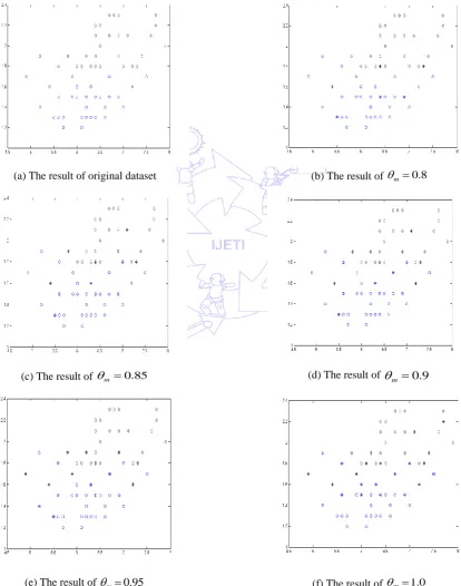
In order to illustrate the behavior of the proposed DCNN algorithm, a set of data points in 2

R space is considered. The numerical values of the prototype data points with five merged rate value of



_m(



_m=0.8, 0.85, 0.9, 0.95 and 1.0) using

the proposed algorithm are listed in Table 1. The simulation results are shown in Fig. 3, where“◇” and“” denote the

positive class and negative class respectively, the data points with“+” inner symbols are prototypes. The results show that

the higher the value of



_m, the larger the number of prototypes, and vice versa. This property makes the DCNN algorithm

flexible to tackle those training samples misclassified in the overlapped region or outliers on the different distributions of

dataset. Thus, we can apply SVM to post-process the set of prototypes from DCNN, to improve the outlier sensitivity

problem of the standard SVM and yield an effectively hybrid classifier.

(a) The result of original dataset (b) The result of



m0.8

(c) The result ofm 0.85 (d) The result of



m 0.9

(e) The result of



_m0.95 (f) The result ofm 1.0

3.3. The GA-DCNN-SVM hybrid model

This section detailed the proposed novel hybrid framework, which integrates the prototype construction, feature

selection and parameter optimization for the SVM. The chromosome representation, fitness definition and system procedure

for the proposed hybrid model are described as follows.

3.3.1. Chromosome Representation

This research used the RBF kernel function (defined by Eq. (7)) for the SVM classifier to implement our proposed

method. The RBF kernel function requires that only two parameters, Cand



should be set. Using the adaptively merged

rate for DCNN and the RBF kernel for SVM, the parameters_m, C,



and features used as input attributes must be optimized simultaneously for our proposed GA-DCNN-SVM hybrid system. The chromosome therefore, is comprised of

four parts,_m, C,



and the features mask. Fig. 5 shows the chromosome representation of our design.

1 2

...

0

,

1 2

...

0

,

1 2

...

0

,

1 2

...

0

m m m

c c r r f f

m m

c c c r r r f f f

n n n n n n n n

b

_{ }

b

_{ }

b



b

_

b

_

b b

_

b

_

b b

_

b

_

b









Fig. 4 Chromosome representation in

m

 ,_C, and features mask

In Fig. 4, 1 ~ 0

m m m n b b   

 indicates the parameter value _m and the bit string’s length is nm, c 1~ 0

c c

n

b  b represents the parameter value C and the bit string’s length is n_c, bn 1~b0

 

 denotes the parameter value



and the bit string’s length

is n_,

1~ 0 f

f f

n

b  b stands for the features mask and nf is the number of features that varies from different datasets.

Furthermore, we can choose different length for each m

n

 ,

n

c and

n

 parameter according to the calculation precision

required.

The bit string b bl₁ l₂...b₀, where bi

 

0,1 ,i0,1,...,l1, representing the genotype format of the parameters m

 ,Cand , should be transformed into phenotype z by Eq. (14). Note that the precision of representing parameter depends on the length of the bit string l (such as

m

n_ , n_cand n_), and the minimum and maximum value [zmin,zmax]

of the parameter is determined by the user. The features mask is Boolean that ‘1’ represents the feature is selected, and ‘0’

indicates the feature is not selected.

1 max min min 0

(

)

2

2

1

l i i l i

z

z

z

z

b

















(14)

3.3.2. Fitness Definition

Fitness function is the guide of GA’s operation to search for optimal solutions. For maximizing the classification

accuracy and minimizing the number of selected features, the fitness function F is a weighted sum with

w

_A for the

classification accuracy weight and

w

_F for the selected features as defined by Eq. (15).

A

_ccis the SVM classification

accuracy, f_iis the value of feature mask－‘1’ represents the feature i is selected and ‘0’ indicates that feature i is not selected, and

n

_f is the total number of features. Thus, for the chromosome with high classification accuracy and a small

number of features produce a high fitness value.

1

1

f n

A F i

i

F w Acc w f





 

   _ _





 (15)

Considering the tradeoff between the classification accuracy and selected feature number, the two weights

w

_A and

F

w

can be adjusted according to the preference of classifier designers. The weight accuracy can be tuned to a high value

Copyright © TAETI

3.3.3. The proposed hybrid GA-DCNN-SVM algorithm

Feature Selection Yes

Prototype Construction (DCNN rule)

SVM Parameter Optimization

GA Operation

Dataset

Testing set Training set

Selected feature subset F GA parameter : feature mask

Testing set with F Training set with F

Training SVM classifier GA parameters : C and r

Learned SVM classifier

Fitness calculation

Optimized Ɵm,C,r and feature subset

Termination check ? GA operation No

Yes Data Preprocessing

Scaling Prototype construction

by PVS algorithm

Merged rate coefficient GA parameter : Ɵm

Merge detection check ? Prototype

Augmentation No

Yes

Fig. 5 The flowchart of the proposed hybrid GA-DCNN-SVM algorithm

Fig. 5 shows the system architecture of our proposed hybrid model. Based on the chromosome representation and

fitness definition mentioned above, detailed descriptions of the novel GA-DCNN-SVM procedure are illustrated as follows.

Procedure GA-DCNN-SVM hybrid model

Step 1: Data preparation

Given a dataset S is considered using the 10-fold cross-validation process to split the data into ten groups. Each

group contains training and testing sets. The training and testing sets are represented as

S

_TRand

S

_TE, respectively.

Step 2: GA initialization and parameters setting

Set the GA parameters including the number of iterations, population sizes, crossover rate, mutation rate, and weight for

fitness calculation. Generate initial chromosomes comprised of the parameters including_m,C,  , and feature mask.

Step 3: Converting genotype to phenotype

Step 4: Prototype construction by using the DCNN algorithm

The DCNN algorithm computes a prototypes subset, denoted by P, from the training set STR according to the merged

rate parameter _m which is represented in the chromosome and calculated from Step 3. Once the prototypes subset P is

computed, the new training set STR' is set to

P

.

Step 5: Scaling

The purpose of feature scaling is to properly describe the interactions between feature attributes and to avoid attributes

in greater numeric ranges dominating those in smaller numeric ranges [3, 14]. Attributewise normalization by Eq. (16) can

be linearly scaled to the range [-1, +1] or [0, 1], where aj( )xi is the original attribute value of feature

x

i, a'j(xi) is

scaled value, max_j and min_j correspond to the maximum and minimum values for attribute aj over all samples.

' ( ) min

( ) ,

max min

j i j

j i

j j

a x

a x   i

 (16)

Step 6: Selected features subset

Select input features for training set STR' and testing set STE according to the feature mask which is represented in

the chromosome from Step 2, then the features subset can be determined. We denote the STR' and STE datasets with

selected features as FSTR' and FSTE, respectively.

Step 7: SVM model training and testing

Based on the parameters C and



which are represented in the chromosome and calculated from Step 3, to train the

SVM classifier on the training dataset FSTR' , then the classification accuracy Acc on the testing dataset FSTE can be

evaluated.

Step 8: Fitness evaluation

For each chromosome, evaluate its fitness value by Eq. (15) when the classification accuracy A_cc is obtained from previous step. The optimal fitness value will be stored to provide feedback on the evolution process of GA to find the

increasing fitness of chromosome in the next generation.

Step 9: Termination check

When the maximal evolutionary epoch is reached, the process ends; otherwise, go to the next step.

Step 10: GA operation

In the evolution process, standard GA operators such as selection, crossover and mutation based on elitist strategy may

be applied to search for better solutions.

4. Experimental Results

4.1. System Implementation Descriptions

To verify the effectiveness of the proposed hybrid system, we tried several real benchmark data sets which are cited

Copyright © TAETI

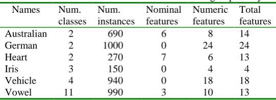
Six real data sets are considered, namely, the Australian data set, the German data set, the Heart disease data set, the Iris

data set, the Vehicle data set, and the Vowel data set. In the above datasets, Table 2 summarizes the number of numeric

attributes, number of nominal attributes, number of classes, and number of instances.

Table 2 Datasets from the UCI Machine Learning Repository Names Num.

classes

Num. instances

Nominal features

Numeric features

Total features

Australian 2 690 6 8 14

German 2 1000 0 24 24

Heart 2 270 7 6 13

Iris 3 150 0 4 4

Vehicle 4 940 0 18 18

Vowel 11 990 3 10 13

The datasets considered are partitioned using the 10-fold cross validation. Each initial data set S, is randomly divided

into ten disjoint sets of equal size T1, …, T10. We maintain the original class distribution (before partitioning) within each set

when carrying out the partition process, and then conduct ten pairs of training and testing sets, ( i TR

S , i

TE

S ), i=1, …, 10. Ten

trials were run for each data set, and the advantage of cross validation is that all of the testing sets were independent and the

reliability of the results could be improved.

Our implementation platform was carried out on Matlab 2013, a mathematical development environment by extending

the LIBSVM which is originally designed by Chang and Lin [16]. The GA-based previously published method by Huang [3],

namely GA-SVM with non-DCNN version, for searching the best C, , and features subset. The existing GA-SVM with

non-DCNN version method deals solely with feature selection and parameters optimization by means of genetic algorithm,

and the treatment of these redundant or noisy instances in a classification process did not taken into account. Our proposed

GA-DCNN-SVM hybrid model has been tested fairly extensively and compared with the non-DCNN version approach using

three criteria, namely, the classification accuracy rate, the number of selected feature, and the non-parametric Wilcoxon

signed rank test. In all of the experiments, 10-fold cross validation was used to estimate the classification accuracy of each

learning algorithm. We report the empirical results in the following section.

4.2. Results and Comparisons

In computation works, we set GA parameters to the same values to compare the performance using the two different

algorithms. The detail parameter setting for GA is as the following: population size 200, generation number 300, crossover

rate 0.7, mutation rate 0.05, two point crossover, roulette wheel selection and the elitism replacement. The bit string’s length

for each parameter nm , nc, n is configured as 20, and the value of nf varies from different datasets described in Table 2. According to the fitness function defined by Eq. (15), set the accuracy’s weight wA0.8 and the feature’s weight

0.2

F

w  for all experiments. The termination criterion is that the generation number achieves generation 300, and the

best chromosome is obtained when the termination criterion satisfies.

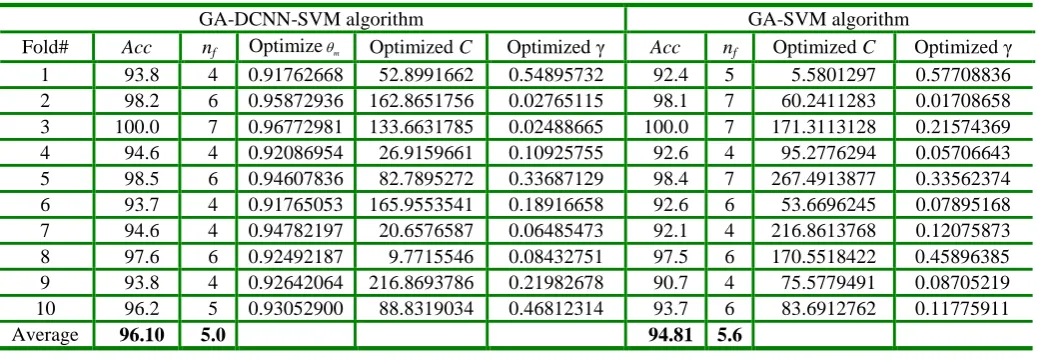
Taking the Heart disease dataset, for example, the classification accuracy Acc, number of selected features nf , and the

best parameters _m, C,



for each fold using GA-DCNN-SVM algorithm and GA-SVM with non-DCNN approach are shown in Table 3. For the GA-DCNN-SVM method, average classification accuracy rate is 96.10%, and average number of

features is 5.0. For the GA-SVM with non-DCNN approach, its average classification accuracy rate is 94.81%, and average

number of features is 5.6. Table 4 shows the summary results for the average classification accuracy rate Avg_Accand the

average number of selected features Avg_nf for the six UCI datasets using the two different approaches. In Table 4, the

be mentioned that in the case of six UCI datasets, the Avg_Acc always increased when the DCNN philosophy was

employed.

Table 3 Experimental results for Heart disease dataset comparison from GA-DCNN-SVM and GA-SVM algorithms

GA-DCNN-SVM algorithm GA-SVM algorithm

Fold# Acc nf Optimizem Optimized C Optimized γ Acc nf Optimized C Optimized γ 1 93.8 4 0.91762668 52.8991662 0.54895732 92.4 5 5.5801297 0.57708836 2 98.2 6 0.95872936 162.8651756 0.02765115 98.1 7 60.2411283 0.01708658 3 100.0 7 0.96772981 133.6631785 0.02488665 100.0 7 171.3113128 0.21574369 4 94.6 4 0.92086954 26.9159661 0.10925755 92.6 4 95.2776294 0.05706643 5 98.5 6 0.94607836 82.7895272 0.33687129 98.4 7 267.4913877 0.33562374 6 93.7 4 0.91765053 165.9553541 0.18916658 92.6 6 53.6696245 0.07895168 7 94.6 4 0.94782197 20.6576587 0.06485473 92.1 4 216.8613768 0.12075873 8 97.6 6 0.92492187 9.7715546 0.08432751 97.5 6 170.5518422 0.45896385 9 93.8 4 0.92642064 216.8693786 0.21982678 90.7 4 75.5779491 0.08705219 10 96.2 5 0.93052900 88.8319034 0.46812314 93.7 6 83.6912762 0.11775911

Average 96.10 5.0 94.81 5.6

To highlight the advantage, the non-parametric Wilcoxon signed rank test is used for all of the datasets. As shown in

Table 4, the p-value for Iris is equal to 1.0, but other p-values are smaller than the statistical significance level of 0.05. Due

to time considerations, the average execution time for GA-DCNN-SVM approach requires more computing time than the

non-DCNN version. It is reasonable that the DCNN rule can achieve optimization merged rate for training data to improve

SVM performance. Generally, compared with the GA-based with non-DCNN version algorithm, the proposed

GA-DCNN-SVM hybrid approach has good classification accuracy performance with fewer features and it effectively

improves the classification accuracy and has fewer input features for support vector machine.

Table 4 Experimental results of GA-DCNN-SVM algorithm and GA-SVM method on six UCI datasets

Name GA-DCNN-SVM GA-SVM p-value for

Wilcoxon testing

_ cc

Avg A Avg_nf Avg_Acc Avg_nf

Australian 90.3±1.42 4.3±0.82 88.2±1.81 4.5±1.08 0.028* German 87.4±0.97 12.6±0.84 85.6±1.80 13.1±1.59 0.022* Heart 96.1±2.32 5.0±1.15 94.8±3.32 5.6±1.26 0.008*

Iris 100±0 1±0 100±0 1±0 1.0

Vehicle 85.9±1.85 8.6±0.97 84.0±2.40 9.7±1.70 0.007* Vowel 99.2±0.75 7.1±0.74 98.5±0.89 7.9±0.88 0.011*

*Statistical significance level is 0.05.

5. Conclusions

In this work, an order-independent algorithm for data reduction, called the Dynamic Condensed Nearest Neighbor

(DCNN) rule, is proposed to adaptively construct prototypes in the training dataset and to reduce the redundant or noisy

instances in a classification process for the SVM. Furthermore, a hybrid model based on the genetic algorithm is proposed to

simultaneously optimize the prototype construction, the feature selection, and the SVM kernel parameters setting for solving

the classification problems. The experimental results illustrate that the proposed method is capable of producing good

classification accuracy with a small number of features on several UCI repository of machine learning datasets. Generally,

the proposed GA-DCNN-SVM hybrid approach outperforms the existing GA-based method without the DCNN scheme and

Copyright © TAETI

learning tasks, such as SVM ensemble strategy constitutes a feasible approach and useful modification of the regular SVM,

is other possible directions to pursue.

Acknowledgment

The authors are thankful to the reviewers for their valuable comments and suggestions.

References

[1] V. N. Vapnik, Statistical learning theory, 1st ed. New York: Wiley, 1998.

[2] D. Anguita, A. Ghio, L. Oneto and S. Ridella, "In-Sample and out-of-sample model selection and error estimation for

support vector machines," IEEE Transactions on Neural Networks and Learning Systems, vol. 23, pp.1390-1406, 2012.

[3] C. L. Huang and C. J. Wang, "A GA-based feature selection and parameters optimization for support vector machines,"

Expert systems with applications, vol. 31, pp. 231-240, 2006.

[4] P. E. Hart, "The condensed nearest neighbor rule," IEEE Transactions on Information Theory, vol. 14, pp. 515-516,

1968.

[5] F. Angiulli and A. Astorino, "Scaling up support vector machines using nearest neighbor condensation," IEEE

Transactions on Neural Networks, vol. 21, pp. 351-357, 2010.

[6] F. Angiulli, "Fast nearest neighbor condensation for Large data sets classification," IEEE Trans. Knowledge and data

engineering, vol. 19, pp. 1450-1464, 2007.

[7] A. Abroudi and F. Farokhi, "Prototype selection for training artificial neural networks based on Fast Condensed Nearest

Neighbor rule," IEEE Conference on Open Systems (ICOS), pp. 1-4, 2012.

[8] X. Zhao, D. Li, Bo Yang, H. Chen, X. Yang, C. L. Yu and S. Y. Liu, "A two-stage feature selection method with its

application," Computers & Electrical Engineering, vol. 47, pp. 114-125, Oct. 2015.

[9] W. Shu and H. Shen, "Incremental feature selection based on rough set in dynamic incomplete data," Pattern

Recognition, vol. 47, pp. 3890-3906, Dec. 2014.

[10] J. R. Rico-Juan and J. M. Iñesta, "Adaptive training set reduction for nearest neighbor classification," Neurocomputing,

vol. 138, pp. 316-324, Aug. 2014.

[11] J. L. Chen and C. S. Yang, "Optimizing the proportion of prototypes generation in nearest neighbor classification,"

International Conference on Machine Learning and Cybernetics (ICMLC), vol. 4, pp. 1695-1699, 2013.

[12] Y. Miao, X. Tao, Y. Sun, Y. Li and J. Lu, "Risk-based adaptive metric learning for nearest neighbor classification,"

Neurocomputing, vol. 156, pp. 33-41, May 2015.

[13] J. H. Holland, Adaption in natural and artificial systems, Cambridge, MIT Press Cambridge, MA, USA, 1992.

[14] X. Sun, J. Wang, F.H. Mary and L. Kong, "Scale invariant texture classification via sparse representation,"

Neurocomputing, vol. 122, pp. 338-348, Dec. 2013.

[15] S. Cateni, V. Colla and M. Vannucci, "A hybrid feature selection method for classification purposes," European

Modelling Symposium (EMS), pp. 39-44, 2014.

[16] C. C. Chang and C. J. Lin, "Training nu-support vector regression: theory and algorithms," Neural Computation, vol. 14,