Learning Trees from Strings: A Strong Learning Algorithm for some
Context-Free Grammars
Alexander Clark [email protected]
Department of Philosophy King’s College London The Strand
London WC2R 2LS
Editor:Mehryar Mohri
Abstract
Standard models of language learning are concerned with weak learning: the learner, receiving as input only information about the strings in the language, must learn to generalise and to generate the correct, potentially infinite, set of strings generated by some target grammar. Here we define the corresponding notion of strong learning: the learner, again only receiving strings as input, must learn a grammar that generates the correct set of structures or parse trees. We formalise this using a modification of Gold’s identification in the limit model, requiring convergence to a grammar that is isomorphic to the target grammar. We take as our starting point a simple learning algorithm for substitutable context-free languages, based on principles of distributional learning, and modify it so that it will converge to a canonical grammar for each language. We prove a corresponding strong learning result for a subclass of context-free grammars.
Keywords: context-free grammars, grammatical inference, identification in the limit, structure
learning
1. Introduction
We present an algorithm for inducing a context-free grammar from a set of strings; this algorithm comes with a strong theoretical guarantee: it works in polynomial time, and for any grammar in a certain class it will converge to a grammar which is isomorphic/strongly equivalent to the target grammar. Moreover the convergence is rapid in a technical sense. This very strong guarantee comes of course at a price: the class of grammars is small. In the first part of the paper we explain the learning model we use which is an extension of the Gold identification in the limit model; and in the second part we present an algorithm which learns a class of languages with respect to this model. We have implemented this algorithm and we present some examples at the end which illustrate the properties of this algorithm, testing on some simple example languages. As far as we are aware this is the first nontrivial algorithm for learning trees from strings which has any sort of theoretical guarantee of its convergence and correctness.
We can contrast the approach here with the task of unsupervised parsing in computational lin-guistics as exemplified by Cohn et al. (2010). Unsupervised parsers use a variety of heuristic ap-proaches to extract a single tree for each sentence, taking as input a large natural language corpus, and being evaluated against some linguistically annotated corpus. Here we are interested not in find-ing the most likely parse, but in findfind-ing the set of allowable parses in a theoretically well-founded way.
1.1 Linguistics
The notions of weak and strong generation are fundamental in the fields of mathematical and the-oretical linguistics. A formal grammar weakly generates a set of strings, and strongly generates a set of structures (Miller, 1999). We do not have the space for a full discussion of the rather subtle methodological and indeed philosophical issues involved with which model is appropriate for study-ing lstudy-inguistics, which questions depend on what the subject matter of lstudy-inguistics is taken to be; we merely note that while mathematical attention has largely focused on the issues of weak generation, many linguists are more concerned with the issues of strong generation and as a result take the weak results to be largely irrelevant (Berwick et al., 2011). Indeed, taking a grammar as a model of human linguistic competence, we are primarily interested in the set of structures generated. Unfortunately, we have little or no direct evidence about the nature of these structures, notwithstanding recent ad-vances in neuroimaging and psycholinguistics, and our sources of information are essentially only about the set of strings that are weakly generated by the grammar, since these can be observed, and our intuitions about the associated meanings.
We can define corresponding notions of weak and strong learning.1 Weak learning involves merely learning a grammar that generates the right set of strings; strong learning involves learning a grammar that generates the right set of structures (Wexler and Culicover, 1980, p. 58). Some sentences are ambiguous and will require a grammar that generates more than one structure for a particular sentence. We do not consider in this paper the problem of learning when the input to the learner aretrees; see for example Sakakibara (1990, 1992), Drewes and H¨ogberg (2003) and L´opez et al. (2004). We consider only the problem where the learner has access to the flat strings alone, but must infer an appropriate set of trees for each string in the language. Rather than observing the derivation trees themselves, we observe only the yields of the trees.
Weak learning of context-free grammars and richer formalisms has made significant progress in recent years (Clark and Eyraud, 2007; Yoshinaka, 2011; Yoshinaka and Kanazawa, 2011; Yoshi-naka, 2012) but strong learning has received less attention. ForCFGs this means that the hypothesis
needs to be isomorphic (assuming it is trim) or better yet,identicalto the target grammar. We define these notions of equivalence and the associated learning models in Section 3. Strong learning is obviously impossible for the full class of context-free grammars since there are an infinite number of structurally different context-free grammars that generate a given context-free language.
In this paper we work in a categorical model which assumes, unrealistically, a partition of the strings into grammatical and ungrammatical, but probabilistically the situation is not better; given a distribution defined by a probabilisticCFG(PCFG) there are infinitely many structurally different
CFGs that define the same set of distributions; in other wordsPCFGs are not identifiable from strings
(Hsu et al., 2013). This is in contrast to discreteHMMs which are (Petrie, 1969).
The contributions of this paper are as follows. We first define an appropriate notion of strong learning from strings, restricting ourselves to the case ofCFGs for simplicity. We then show that ex-isting learning algorithms for regular languages (Angluin, 1982) can be viewed as also being strong learning algorithms, in a trivial sense. We then present a strong learning algorithm for someCFGs,
based on combining the polynomial algorithm for substitutable context-free languages defined in Clark and Eyraud (2007), which we recall in Section 4, with a recent proposal for a formal notion of syntactic structure (Clark, 2011) that we interpret as a form of canonical grammars. We spec-ify the canonical grammars we target in Section 5, present an algorithm in Section 6, and prove its correctness and efficiency in Section 7. Section 8 contains some examples, including one with an ambiguous grammar. An appendix contains some detailed proofs of various technical lemmas regarding the properties of the languages we consider in this paper.
2. Notation
LetΣ be a finite non-empty set of atomic symbols. Σ∗ is the set of all finite strings over Σ. We denote the empty string byλ. The set of non-empty strings isΣ+=Σ∗\ {λ}. We write|u|for the length of a stringu, and for a finite set of stringsXwe define the size askXk=∑w∈X|w|.
A languageLis any subset ofΣ∗. Given two languagesM,N⊆Σ∗we writeM·Nor sometimes justMN for the set{uv|u∈M,v∈N}. Note that this is just the normal concatenation of sets of strings.
Given a languageD, we define Sub(D)to be the set of non-empty substrings of elements ofD:
Sub(D) ={u∈Σ+| ∃(l,r)∈Σ∗×Σ∗,lur∈D}.
Given a non-zero sequence of languagesα=hX1, . . . ,Xniwe write ¯αfor the concatenation, that
is, ¯α=X1· · · · ·Xn. We shall assume an order≺oron Σwhich we shall extend to the
length-lexicographic order onΣ∗.
We define a context(l,r)to be an ordered pair of strings, an element ofΣ∗×Σ∗. The distribution of a stringu∈Σ∗with respect to a languageLis defined to be
DL(u) ={(l,r)∈Σ∗×Σ∗|lur∈L}.
We say that u≡Lv iff DL(u) =DL(v). This is the syntactic congruence, which is equivalent to
complete mutual substitutability ofuandv.
We write[u]Lfor{v∈Σ∗|DL(u) =DL(v)}. If we have a set of strings,X, that are all congruent
then we write[X]for the congruence class containing them. Note that for any stringsu,v, [uv]⊇
[u][v]so ifX,Y are congruence classes we can write[XY]and the result is well defined.
The unique congruence class[λ]is called the unit congruence class. The set {u|DL(u) = /0}
if it is non-empty is a congruence class, which is called the zero congruence class. A congruence class in a languageLis non-zero iff it is a subset of Sub(L). We are mostly concerned with non-zero non-unit congruence classes in this paper.
Definition 1 We will be considering sequences of congruence classes: so ifαis a sequence X1, . . . ,Xn
where each of the Xiis a congruence class, then we writeα¯ for the set of strings formed by
concate-nating all of the Xi. We write|α|for the length of the sequence, n in this case. Note that all of the
elements ofα¯ will be congruent: if u,v∈α¯ then u≡Lv. We can therefore write without ambiguity
We say thatu=.Lvif there is some(l,r)such thatlur∈Landlvr∈L. This is partial or weak
substitutability;uandvcan be substituted for each other in the context(l,r). Ifu≡Lvandu,vhave
a non-empty distribution thenu=.Lv, but the converse is clearly not true.
Definition 2 A language L issubstitutableif for all u,v∈Σ+, u=.Lv implies u≡Lv.
In other words, for any two non-empty strings u,vif DL(u)∩DL(v)6= /0then DL(u) =DL(v).
This language theoretic closure property allows us to define algorithms that generalise correctly, even under pessimistic learning conditions.
2.1 Context-Free Grammars
A context-free grammar (CFG) G is a tuple G=hΣ,V,I,Pi whereV is a finite non-empty set of nonterminals disjoint from Σ, I ⊆V is a set of distinguished start symbols and P is a subset of V×(V∪Σ)+ called the set of productions. We write this asN→α. We do not allow productions with a right hand side of length 0, and as a result the languages we consider will not contain the empty string. We use
G
CFGfor the class of all context-free grammars.We define the standard notion of single-step derivation as ⇒ and define ⇒∗ as the reflexive transitive closure of⇒; for all N∈V,
L
(G,N) ={w∈Σ∗|N⇒∗ w}; andL
(G) =SS∈IL
(G,S). Using a set of start symbols rather than a single start symbol does not change the generative capacity of the formalism.We say that a CFGis trim if for every nonterminalN there is a context(l,r)such thatS⇒∗ lNr for someS∈Iand a stringusuch thatN⇒∗ u: in other words every nonterminal can be used in the derivation of some string.
We say that twoCFGs,GandG′are weakly equivalent if
L
(G) =L
(G′).Proposition 3 (Ginsburg, 1966) Given two CFGs, G and G′, it is undecidable whether
L
(G) =L
(G′).Two CFGs are isomorphic if there is a bijection between the two sets of nonterminals which extends to a bijection between the productions. In other words they are identical up to a relabeling of nonterminals. We denote this byG∼=G′. Clearly if two grammars are isomorphic then they are weakly equivalent.
Proposition 4 Given twoCFGs, G and G′, it is decidable whether G∼=G′.
There is a trivial exponential time algorithm that involves searching through all possible bijec-tions. This problem is GI-complete: as hard as the problem of graph isomorphism (Zemlyachenko et al., 1985; Read and Corneil, 1977). We may not be able to do this efficiently for generalCFGs.
3. Learning Models
We start by reviewing the basic theory of learnability using the Gold identification in the limit paradigm (Gold, 1967). We consider only the model of given text—where the learner is provided with positive data only. We assume a class ofCFGs,
G
⊆G
CFG.A presentation of a language Lis an infinite sequence of elements ofΣ∗,w1,w2, . . . such that
of the firstnelements. A polynomial learning algorithm is a polynomially computable function from finite sequences of positive examples to
G
CFG.Given a presentationT of some languageL, we can applyAto the various prefixes ofT, which produces an infinite sequence of elements of
G
CFG,A(T1),A(T2), . . .. These are hypothesisgram-mars; we will useGito refer toA(Ti), theith hypothesis output by the learning algorithm.
Consider a target grammarG∗∈
G
, and a sequence of hypothesized grammarsG1,G2, . . .pro-duced by a learning algorithm on a presentationT for
L
(G∗). There are various notions of conver-gence of which we outline four, which vary on two dimensions: one dimension concerns whether we are interested in weak or strong learning, and the other whether we are interested in controlling the number of internal changes as well, or are only interested in the external behaviour.Weak behaviorally correct learning (WBC)
There is anNsuch that for alln>N,
L
(Gn) =L
(G∗).Weak Gold learning (GOLD)
There is anNsuch that for alln>N,
L
(Gn) =L
(G∗)andGn=GN.Strong behaviorally correct learning (SBC) There is anNsuch that for alln>N,Gn∼=G∗.
Strong Gold learning (SGOLD)
There is anNsuch that for alln>N,Gn=∼G∗andGn=GN.
For each of these four notions of convergence, we have a corresponding notion of learnabil-ity. We say that a learner, A, WBC/GOLD/SBC/SGOLD learns a grammar G∗, iff for every pre-sentation of
L
(G∗), it WBC/GOLD/SBC/SGOLD converges on that presentation. Given a class ofCFGs,
G
, we say thatAWBC/GOLD/SBC/SGOLDlearns the class, iff for everyG∗ inG
the learnerWBC/GOLD/SBC/SGOLDlearnsG∗.
In the case of GOLD learning, this coincides precisely with the standard model of Gold iden-tification in the limit from given text (positive data only) (Gold, 1967). WBC-learning is the
stan-dard model of behaviorally correct learning (Case and Lynes, 1982). We cannot in general turn a
WBC-learner into aGOLD-learner: see discussion in Osherson et al. (1986). The property of order-independenceas defined by Blum and Blum (1975), can be thought of as an even stronger version ofSGOLDlearning.
However, aSBC-learner can be changed into aSGOLD-learner, if we can test whether two hy-potheses are isomorphic. There does not seem to be a theoretically interesting difference between
SBC-learning andSGOLD-learning: the only difference, in the case ofCFGs, is that theSBC learner may occasionally pick different labels for the nonterminals after convergence, whereas theSGOLD
learner may not.
We can ask how can aGOLDlearner differ from aSGOLDlearner: how can a weak learner fail to be a strong learner? The difference is that on different presentations of the same language, a weak Gold learner may converge to different answers. That is to say we might have a learner which on presentationT′of grammarGproduces a grammarG′and on presentationT′′of the same grammar, produces a grammarG′′, whereG′andG′′are weakly equivalent but not isomorphic.
Proposition 6 Suppose that A is an algorithm whichSGOLD-learns a class of grammars
G
. ThenG
is not redundant.The proof is immediate—any presentation forG1is also a presentation forG2. In other words
if
G
contains two non-isomorphic grammars for the same language then it is not strongly learnable. A simple corollary is then that the class ofCFGs is not strongly identifiable in the limit even frominformed data, that is to say from labelled positive and negative examples, since there are an infinite number of non-isomorphic grammars for every non-empty language.
One can therefore try to convert a weak learner to a strong learner by defining a canonical form. If we can restrict the class so that there is only one structurally distinct grammar for each language, and we can compute that, then we could find a strong learning algorithm. We formalise this as follows. SupposeAis some learning algorithm that outputs grammars in a hypothesis class
H
A⊆G
CFG, and suppose that it canGOLD-learn the class of grammarsG
⊆H
A. Suppose we havesome ‘canonicalisation’ functionffrom
H
A→G
CFGsuch that for eachG∈G
,L
(G) =L
(f(G))andsuch thatf(
G
)is not redundant. Then we can construct a learnerA′which outputsA′(Ti) =f(A(Ti)),which will then be aSGOLDlearner for
G
. Moreover, ifAand f are both polynomially computable then so willA′ be.For example, suppose
D
is the class of allDFAs and fis the standard function for minimizing a deterministic finite-state automaton (DFA), which can be done in polynomial time. Since all minimal DFAs for a given regular language are isomorphic, f(D
)is not redundant. Therefore any learner for regular languages that outputsDFAs, such as the one in Angluin (1982), can be converted into a strong learner using this technique. From the point of view of structural learning such results are trivial in two important respects. The first is that each string in the language has exactly one labelled structure, and the other is that every structure is uniformly right branching, whereas we are interested in learning grammars which may assign more than one different structure to a given string.Moreover, it is easy to see that any SGOLD-learner for a class of grammars
G
will implicitly define such a canonicalisation function forG
. We can enumerate the strings in the language and apply the learner to them, and the limit of the hypothesis grammars will then satisfy the conditions given above, though this function may not be computable. There is therefore a close relationship between canonicalisers and strong learners. There is much more that could be said about the learning models, and further refinements of them, but this is enough for our purposes.4. Weak Learning of Substitutable Languages
We recall the Clark and Eyraud (2007) result, using a simplified version of the algorithm (Yoshinaka, 2008), and explain why it is only a weak rather than a strong result.
Given a finite non-empty set of strings D={w1, . . . ,wn}the learner constructs a grammar as
shown in Algorithm 1. We create a set of symbols in bijection with the elements of Sub(D)where we write[[u]]for the symbol corresponding to the substringu: that is to say we have one nonterminal for each substring of the observed data. The grammar ˆG(D) is the CFG hΣ,V,I,PL∪PB∪PUi as
shown in the pseudocode in Algorithm 1. The setsPL,PBandPU are the sets of lexical, branching
and unary productions respectively.
Algorithm 1Grammar construction procedure
Data: A finite set of stringsD={w1,w2, . . . ,wn} Result: ACFGG
V:=Sub(D); I:={[[u]]|u∈D};
PL:={[[a]]→a|a∈Σ∩V};
PB:={[[uv]]→[[u]][[v]]|u,v,uv∈V};
PU:={[[u]]→[[v]]| ∃(l,r)∧lur∈D∧lvr∈D};
outputG=hΣ,V,I,PL∪PB∪PUi
c}, PB ={[[ac]]→[[a]][[c]],[[cb]]→[[c]][[b]],[[acb]]→[[ac]][[b]],[[acb]]→[[a]][[cb]]} and PU =
{[[c]]→[[acb]],[[acb]]→[[c]]}. As can be verified thisCFGdefines the language{ancbn|n≥0}.
There are two natural ways to turn this grammar construction procedure into a learning algo-rithm. One is simply to apply this procedure to all of the available data. This will give aWBC-learner for the class of substitutableCFGs.
Alternatively since we can parse with the grammars, we can convert this into a GOLDlearner,
by only changing the hypothesis when the hypothesis is demonstrably too small. This means that once we have a weakly correct hypothesis the learner will no longer change its output. This simple modification gives a variant of the learner in Clark and Eyraud (2007). However this does not mean that this is a strong learner, since it may converge to a different hypothesis for different presenta-tions of the same language. For example if a presentation of the language from Example 1 starts
{a,acb, . . .}then the learner will converge in two steps to the grammar shown in Example 1. If on the other hand, the presentation starts{acb,aacbb, . . .}then it will also converge in two steps, but to a different, larger, grammar that includes nonterminals such as[[aa]]and has a larger set of productions. This grammar is weakly equivalent to the former grammar, but it is not isomorphic or structurally equivalent, as it will assign a larger set of parses to strings likeaacbb. It is more ambiguous. Indeed it is easy to see that this grammar will assign every possible binary branching structure to any string that is part of the set that the grammar is constructed from. And of course, the presentation could start with an arbitrarily long string—in which case the first grammar which it generates could be arbitrarily large.
5. The Syntactic Structure of Substitutable Languages
In this section we use a modification of Clark (2011) as the basis for our canonical grammars; in the case of substitutable languages the theory is quite simple so we will not present it in all its generality. Each nonterminal/syntactic category will correspond to a congruence class. With substitutable languages, we can show that the language itself, considered as a set of strings, has a simple intrinsic structure that can be used to define a particular finite grammar.
We start with the following definition:
In other words a class is not prime if it can be decomposed into the concatenation of two other congruence classes. The stipulation that the unit and zero congruence classes are not prime is analogous to the stipulation that 1 is not a prime number. We will not give a detailed exposition of why the concept of a prime congruence class is important, but one intuitive reason is this. If we have nonterminals that correspond to congruence classes, and a congruence classN is composite, then that means that we can decomposeNinto two classesP,Qsuch thatN=PQ. In that case we can replace every occurrence ofNon the right hand side of a rule by the sequencehP,Qi; assuming that PandQcan be represented adequately, nothing will be lost. Thus non-prime congruence classes can always be replaced by a sequence of prime congruence classes, and we can limit our attention to the primes which informally are those where “the whole is greater than the sum of the parts”. More algebraically, we can think of the primes as representing the points where the concatenation operations in the free monoid and the syntactic monoid differ in interesting ways.
Example 2 Consider the language L={ancbn|n≥0}. This language is not regular and therefore has an infinite number of congruence classes of which three are prime. The congruence classes are as follows:
• {λ}is a congruence class with just one element; this is the unit congruence class which is not prime.
• The zero congruence class which consists of all strings that have empty distribution.
• L is a congruence class which is prime.
• [a] ={a}is prime as is[b] ={b}.
• We also have an infinite number of congruence classes of the form{ai}for any i>1. These are all composite as they can be represented as[a]·[ai−1]; similarly for{bi}.
• Similarly we have classes of the form[aic] ={ai+jcbj| j≥0}and[cbi] ={ajcbi+j |j≥0}
which again are composite.
Lis not always prime as the following trivial example demonstrates.
Example 3 Consider the finite language L={ab}. This language has 5 congruence classes:
[a],[b],[ab],[λ]and the zero congruence class. The first 4 are all singleton sets. [a] and[b]are prime but[ab] ={ab}= [a][b], and so L is not prime.
Proposition 8 For every a∈Σ, for any language L, if[a]is non-zero and non-unit then[a]is prime.
Proof Letabe some letter in a languageLand let[a]be its congruence class. Suppose there are two congruence classesX,Y such thatXY = [a]. Sincea∈[a],amust be inXY. Since we cannot split a string of length 1 into two non-empty strings, one ofX andY must be the unit.
We can now define the class of languages that we target with our learning algorithm.
Given that there are substitutable languages which are notCFLs—theMIXlanguage (Kanazawa and Salvati, 2012) being a good example—we need to restrict the class in some way. Here we consider only languages where there are a finite number of prime congruence classes. This implies, as we shall see later, that the language is a CFL. Every regular language of course has a finite
number of primes as it has a finite number of congruence classes. Not all substitutable context-free languages have a finite number of primes, as this next example shows.
Example 4 Consider the language L={cibaib|i>0} ∪ {cideid|i>0}. This is a substitutable context-free language. The distribution of baib is the single context{(ci,λ)}which is the same as
that of deid. Therefore we have an infinite number of congruence classes of the form{baib,deid}, each of which is prime.
Definition 10 Aprime decompositionof a congruence class X is a finite sequence of one or more prime congruence classesα=hX1, . . . ,Xkisuch that X =α¯.
Clearly any prime congruence classX has a trivial prime decomposition of length one, namely
hXi. We have a prime factorization lemma for substitutable languages; we can rather pompously call this the ‘fundamental lemma’ by analogy with the fundamental lemma of arithmetic. This lemma means that we can represent all of the congruence classes exactly using just concatenations of the prime congruence classes.
Lemma 11 Every non-zero non-unit congruence class of a language in
L
sc has a unique primefactorisation.
For proof see Lemma 33 in the appendix. Note that this is not the case in general for languages which are not substitutable, as the following example demonstrates.
Example 5 Let L={abcd,apcd,bx}. Note that L is finite but not substitutable since p6≡b. Among the congruence classes are {a},{b},{c} {ab,ap}, {bc,pc} and {abc,apc}. Clearly {ab,ap},
{bc,pc}are both prime but{abc,apc}is composite and has the two distinct prime decompositions
{ab,ap} · {c}and{a} · {bc,pc}.
If we restrict ourselves to languages in
L
sc then we can assume without loss of generality thatthe nonterminals of the generating grammar correspond to congruence classes. In a substitutable language, a trimCFGcannot have a nonterminal that generates two strings that are not congruent. Similarly, if the grammar had two distinct nonterminals that generated congruent strings, we could merge them without altering the generated language.
Given that non-regular languages will have an infinite number of congruence classes, and that
CFGs have by definition only a finite number of nonterminals, we cannot have one nonterminal for every congruence class. However in languages in
L
sc there are only finitely many prime5.1 Productions
We now consider an abstract notion of a production where the nonterminals are the prime congru-ence classes.
Definition 12 Acorrectbranching production is of the form[α¯]→αwhere αis a sequence of at least 2 primes and[α¯]is a prime congruence class. A correct lexical production is one of the form
[a]→a where a∈Σ, and[a]is prime.
Example 6 Consider the language L={ancbn|n≥0}. This has primes[a],[c]and[b]. The correct lexical productions are the three obvious ones [a]→a, [b]→b and [c]→c. The only correct branching productions have[c]on the left hand side, and are[c]→[a][c][b],[c]→[a][a][c][b][b]and so on.
Clearly in the previous example we want to rule out productions like[c]→[a][a][c][b][b]since the right hand sides are too long, and will make the derivation trees too flat. We want each pro-duction to be as simple as possible. Informally we say that the right hand side of the propro-duction
[a][a][c][b][b]is too long since there is a proper subsequence [a][c][b]which generates strings in a prime congruence class, and should be represented just by the prime[c].
Definition 13 We say that a sequence of primesαispleonastic(too long) ifα=γβδfor someγ,β,δ, which are sequences of primes, such that|γ|+|δ|>0,[β¯]is a prime, and|β|>1.
Definition 14 We say that a correct production N→αispleonastic ifα is pleonastic. A correct production isvalidif it is not pleonastic.
Note that a pleonastic production by definition must have a right hand side of length at least 3. For any string w in a prime congruence class where w=a1. . .an, ai ∈Σ we can construct
a correct production [w]→[a1]. . .[an]. Such productions may in general be pleonastic because
there may be substrings that can be represented by prime congruence classes. From a structural perspective, the local trees derived from these productions are too shallow as they flatten out relevant parts of the structure of the string. Nonetheless we can find a set of valid productions that will generate the stringwfrom the nonterminal[w], as Lemma 18 below shows.
5.2 Canonical Grammars
We will now define canonical grammars for every languageLin
L
sc. Note that for every languagein
L
sc,Lis a congruence class.First of all we need the following lemma to establish that the grammar will be finite: see proof of Lemma 35 in the appendix.
Lemma 15 If L∈
L
scthen there are a finite number of valid productions.• the single production containing the start symbol: S→α(L),
• all valid productions, of which there are only finitely many by Lemma 15,
• for each terminal symbol a that occurs in the language, the production[a]→a.
This is a uniqueCFGfor every language in
L
sc. We now show thatG∗(L)generatesL.Lemma 17 If L ∈
L
sc is a substitutable language, then for any prime congruence class X ,L
(G∗(L),X)⊆X .Proof This is a simple induction on the length of the derivation. ForX→a, we know thata∈X by construction. SupposeXi⇒∗ uifor all 1≤i≤nandX0→X1. . .Xnis a production in the grammar.
Then by the inductive hypothesisui∈Xiand by the correctness of the production,u1. . .un∈X0.
Lemma 18 Suppose X→αis a correct production. Then X ⇒∗G∗(L)α.
Proof By induction on the length ofα. Base case: α is of length 2, in which case it cannot be pleonastic, and soX →α is valid and inG∗(L), and thereforeX⇒∗ α. Inductive step: consider a correct production X →α where α is of lengthk. If it is not pleonastic, then it is valid, and so X→αis a production inG∗(L), and soX⇒∗ α. Alternatively it is pleonastic and thereforeα=βγδ whereγis the right hand side of a correct production,Y →γ. ConsiderX→βYδ, andY →γ. Both
βYδandγare shorter thanα, and so by the inductive hypothesisX⇒∗ βYδandY ⇒∗ γsoX⇒∗ α. So the lemma follows by induction.
Lemma 19 Suppose X is a prime, and w∈X . Then X⇒∗G∗(L)w.
Proof Ifwis of length 1, then we haveX →w. Letw=a1. . .an be some string of lengthn>1.
Letα= [a1]. . .[an]. SoX→αis a correct production. Therefore by Lemma 18X⇒∗ α. Since we
have the lexical rules[ai]→aiwe can also deriveα⇒∗ w.
Proposition 20 For any L∈
L
sc,L
(G∗(L)) =L.Proof SupposeLhas prime factorisationA1. . .An.Soccurs on the left hand side of the single
pro-ductionS→A1. . .An. Since
L
(G∗(L),Ai) =Aiby Lemmas 17 and 19,L
(G∗(L),S) =A1. . .An=L.Definition 21 We define
G
scto be the set of canonical context-free grammars for the languages inL
sc:G
sc={G∗(L)|L∈L
sc}.Lemma 22
G
scis not redundant.Proof Suppose we have two weakly equivalent grammars G1,G2 in this class; then G1 =
6. An Algorithm for Strong Learning
We now present a strong learning algorithm. We then demonstrate in Section 7 that for all grammars in
G
scthe algorithm strongly converges in theSGOLDframework.In outline, the algorithm works as follows; we accumulate all of the data that we have seen so far into a finite setD. We start by using Algorithm 1 to construct aCFGGw which will be weakly correct for a sufficiently large input data. Using this observed data, together with the grammar which is used for parsing, we can then compute the canonical grammar for the language as follows.
1. We partition Sub(D)into congruence classes, with respect to our learned grammarGw.
2. We pick the lexicographically shortest string in each class as the label we will use for the nonterminal.
3. We then test to see which of the congruence classes are prime.
4. Each class is decomposed uniquely into a sequence of primes.
5. A set of valid rules is constructed from the strings in the prime congruence classes.
6. We then eliminate pleonastic productions from this set of productions.
7. Finally, we return a grammarGsconstructed from these productions.
We can perform the first task efficiently, using the grammar and the substitutability property. Given that each string in Sub(D)occurs in the sampleD, for each substringuwe have some context
(l,r)such that lur∈D. Given the substitutability condition, v is congruent touiff lvr∈
L
(G∗). Under the assumption that the grammar is correct we can test this by seeing whetherlvr∈L
(Gw), using a standard polynomial parser, such as a CKY parser.We now have a partition of Sub(D) into k classes C1, . . . ,Ck. We pick the lexicographically
shortest element of each class (with respect to ≺) which we denote by u1, . . . ,uk. Given a class,
we want to test whether it is prime or not. Take the shortest elementw in the class. Test every possible split of winto non-zero strings u,v such thatuv=w. Clearly there are |w| −1 possible splits—for each split, identify the classes ofu,vand test to see whether every element in the class can be formed as a concatenation of these two. If there is some string that cannot be split, then we know that the congruence class must be prime. If on the other hand we conclude that the class is not prime, we might potentially be wrong: we might for example think thatX=Y Zsimply because we have not yet observed one of the strings inX\Y Z. We present the pseudocode for this procedure in Algorithm 2.
For all of the non-prime congruence classes, we now want to compute the unique decomposition into primes. There are a number of obvious polynomial algorithms. We start by taking the shortest stringwin a class; suppose it is of lengthnconsisting ofa1. . .an. We convert this into a sequence
of primes [a1]. . .[an]. We then greedily convert this into a unique shortest sequence of primes
Algorithm 2Testing for primality
Data: A set of stringsX
Data: A partition of strings
X
={X1, . . . ,Xn}, such that Sub(X)⊆SX
Result: True or falseSelect shortestw∈X;
foru,v∈Σ+such thatuv=wdo
Xi∈
X
is the set such thatu∈Xi;Xj∈
X
is the set such thatv∈Xj; if X⊆XiXj thenreturn false;
end if end for
return true;
primes by looking at the primes of the relevant segments. Note that since the lexical congruence classes are all prime, we know there will be at least one such path; since the language is substitutable we know this will be unique.
We then identify a set of valid productions. Every valid production will be of the formN→Mα
whereN,Mare primes andαis a prime decomposition of length at least 1. For any givenN,Mthere will be at most one such rule. Accordingly we loop through all triples ofN andM,Qas follows: for each primeN, for each primeM, for each classQ, takeαto be the prime decomposition ofQ, and test to see ifN→Mαis valid. We can test if it is correct easily by taking any shortest string ufromMand any shortest string vfromαand seeing ifuv∈N; if it does then the rule is correct. Then we can test if it is valid by taking every proper prefix ofMαof length at least two and testing if it corresponds to a prime. If no prefix does then the production is not pleonastic and is therefore valid.
For the lexical productions, we simply add all productions of the form[a]→awherea∈Σ. For the initial symbolS, we identify the unique congruence class of strings in the languageX. If it is prime, then we add a ruleS→X. If it is not prime, andαis its unique prime decomposition then we add the ruleS→α.
7. Analysis
We now proceed to the analysis of Algorithm 3, the learner
A
SGOLD. We want to prove three things:first that the algorithm strongly learns a certain class; secondly, that the algorithm runs in polyno-mial update time; finally that the algorithm converges rapidly, in the technical sense that it has a polynomially sized characteristic set.
We now are in a position to state our main result. We have defined a learning model,SGOLD, an algorithmASGOLDand a class of grammars
G
sc.Theorem 23 ASGOLD SGOLD-learns the class of grammars
G
sc.Algorithm 3
A
SGOLDStrong Gold Learning Algorithm Data: A sequence of stringsw1,w2, . . .Data:Σ
Result: A sequence ofCFGsG1,G2, . . .
letD:=∅; forn=1,2, . . .do
letD:=D∪ {wn};
ˆ
G=Gˆ(D);
LetCbe the partition of Sub(D)into classes;
LetPrbe the set of primes computed using Algorithm 2;
For each classNinCcompute the prime decompositionα(N)∈Pr+;
LetV ={[[N]]|N ∈Pr} be a set of nonterminals each labeled with the lexicographically shortest element in its class;
LetSbe a start symbol;
PL={[[N]]→a|[[N]]∈V,a∈Σ∩N};
PI={S→[[N]]| ∃w∈N,w∈D};
PB=/0;
forN∈Pr,M∈Pr,Q∈Cdo
R= (N→Mα(Q));
ifRis correct and validthen
PB=PB∪ {R}; end if
end for
outputGn:=hΣ,V∪ {S},{S},PL∪PB∪PIi; end for
a sufficiently large, yet polynomially bounded set of strings from
L
(G∗)such that when the input data includes this set, the weak grammar output will be correct (Clark and Eyraud, 2007) and which contains the shortest string in each prime congruence class.Definition 24 For a grammar G=hΣ,V,I,Piwe defineχ(G)as follows. For anyα∈(Σ∪V)+we define w(α)∈Σ+ to be the smallest word, according to≺, generated byα. Thus in particular for any word u∈Σ+, w(u) =u. For each non-terminal N∈V define c(N)to be the smallest pair of terminal strings(l,r)(extending≺fromΣ∗ toΣ∗×Σ∗, in some way), such that S⇒∗ lNr. We now define the characteristic setχ(G∗) ={lwr|(N→α)∈P,(l,r) =c(N),w=w(α)}.
We prove the correctness of the rest of the model under the assumption that the input data containsχ(G∗)and as a result thatGw is weakly correct:
L
(Gw) =L
(G∗). First, ifGw is correct, then the partition of Sub(D)into congruence classes will be correct in the sense that two strings of Sub(D)will be in the same class iff they are congruent.Lemma 25 Suppose X1, . . . ,Xn is a correct partition ofSub(D)into congruence classes. Then if
Algorithm 2 returns true when applied to Xi, then[Xi]is in fact prime.
Proof Suppose[Xi]is not prime: then there are two congruence classesY,Z such that[Xi] =Y Z.
w∈Sub(D),u,v∈Sub(D). Since the partition of Sub(D)is correct, there must be setsXj,Xk such
thatu∈Xj,v∈Xk. Therefore, using again the correctness and the fact that Sub(D) is substring
closed, we have thatXi⊆XjXk, in which case Algorithm 2 will return false.
Lemma 26 Suppose X1, . . . ,Xnis a correct partition ofSub(D)into congruence classes, and D⊇ χ(G∗). Then Algorithm 2 returns true when applied to Xi, iff[Xi]is in fact prime.
Proof Xi is a finite subset of Sub(D), and we assume that all of the elements ofXiare in fact
con-gruent. We already showed one direction, namely that if the algorithm returns true then[Xi]is prime
(Lemma 25). We now need to show that if[Xi]is prime, then the algorithm correctly returns true.
If[Xi]is prime, then it will correspond to some nonterminal in the canonical grammarG∗, sayN. There will be more than one production inG∗withNon the left hand side, and so by the construc-tion ofχ(G∗), and the correctness of the weak grammar, we will have at least one string from each production in Sub(D), which means that since it is a correct partition the algorithm cannot find any pair of classes whose concatenation containsXi.
As a consequence of this Lemma, we know that the algorithm will be able to correctly identify the set of primes of the language, and as a result will converge to the right set of nonterminals.
Proposition 27 If the input data includesχ(G∗), then Gs∼=G∗.
Proof We can verify that all and only the valid productions will be generated by the algorithm by the construction of the characteristic set.
Suppose N→X1. . .Xn is a valid production in the grammar. Then by the construction of the
characteristic set we will have a unique congruence class in the grammar corresponding to[X2· · ·Xn].
Ifn>2 then this will be composite, and if n=2 this will be prime, but in any event it will have a unique prime decomposition which will be exactlyhX2, . . . ,Xni, by Lemma 33. Therefore this
production will be produced by the algorithm.
Secondly suppose the algorithm produces some production N→X1, . . .Xn. We know that this
will be valid sinceX2, . . .Xnis a prime decomposition and is thus not pleonastic, and we tested all
of the prefixes. We know that it will be correct, by the correctness of the weak learner and the fact that the congruence classes are correctly divided. It is easy to verify that the lexical and initial rules are also correctly extracted.
To conclude the proof of Theorem 23, we just need to observe that since the characteristic set includes the shortest element of each prime congruence class, and so the labels for each nonterminal will not change which means that the output grammars will converge exactly.
S→NT0 NT1→b NT2→a NT0→c
NT0→NT2 NT0 NT1
S→NT0 NT3→open NT2→close NT4→neg NT4→NT0 NT1 NT0→a
NT0→b NT0→c
NT0→NT3 NT4 NT0 NT2 NT1→and
NT1→iff NT1→implies NT1→or
S→NT0
NT2→NT2 NT0 NT2→NT0 NT2 NT2→a
NT0→NT0 NT0 NT0→NT2 NT1 NT0→NT1 NT2 NT1→b
NT1→NT1 NT0 NT1→NT0 NT1
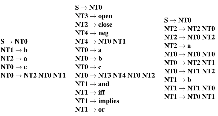
Table 1: Output grammars for the three examples; on the left the grammar for{ancbn|n≥0}, in the middlem the language of propositional logic, and on the right, the ambiguous grammar for{w∈ {a,b}+| |w|
a=|w|b}.
8. Examples
We have implemented the algorithm presented here.2 We present the results of running this al-gorithm on small data sets that illustrate the properties of the canonical grammars for the learned languages. These examples are not intended to demonstrate the effectiveness of the algorithm but merely as illustrative examples to help the reader understand the representational assumptions, and as a result we have restricted ourselves to very simple languages which will be easy to understand. Nonterminals in the output grammar are eitherSfor the start symbol orNTfollowed by a digit for the congruence classes that correspond to primes.
8.1 Trivial Context-Free Language
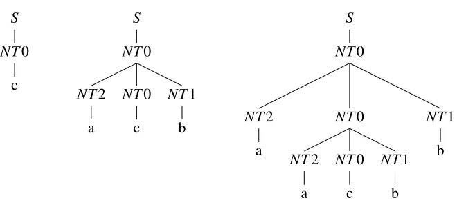
Consider the running example of {ancbn|n≥0}. A characteristic set for this is just {c,acb}. Given this input data, we get the grammar shown on the left of Table 1. This defines the correct language; Figure 1 shows the parse trees for the three shortest strings in the language. This grammar is unambiguous so every string has only one tree.
8.2 Propositional Logic
Our next example is the language of sentential logic, with a finite number of propositional symbols. We have the alphabet {A1, . . . ,Ak,(,),¬,∨,∧,⇒,⇔}. We would standardly define this language
with the CFG: S →Ai, S →(¬S), S→ (S∨S), S →(S∧S), S→(S⇒S) and S→(S⇔S).
Note that in this language the brackets are part of the object language not the meta-language—the algorithm does not know that they are brackets or what their function is. We replace them with other symbols in the experiment to emphasize this point. Thus the algorithm is given only flat sequences
S
NT0
c
S
NT0
NT2
a
NT0
c
NT1
b
S
NT0
NT2
a
NT0
NT2
a
NT0
c
NT1
b
NT1
b
Figure 1: Example parse trees for the example{ancbn|n≥0}.
of strings—there is implicitly structural information here, but the algorithm must discover it, as it must discover that the correct grammar is unambiguous. Sentential logic is an interesting example because it illustrates a case where the algorithm works but produces a different parse tree, but one that is still adequate for semantic interpretation. The canonical structure does not look like the ancestral tree we would see in a textbook presentation (Enderton, 2001).
Since(¬A)and(A∨A)are both in the language,¬ ∼=A∨, so the parse tree for(A∨B)will look a little strange: the canonical grammar has pulled out some more structure than the textbook grammar does: see Figure 2 for example trees. Nonetheless this is still suitable for semantic interpretation and the grammar is still unambiguous.
We fix some input data, replacing the symbols with strings to obtain input data of{a, b, c, open a and b close, open a or b close, open a implies c close, open a iff c close, open neg a close}. This produces the grammar shown in the middle of Table 1, which is weakly correct. This generates one tree for each string in the language as shown in Figure 2.
8.3 An Ambiguous Language
The next example is the language which consists of equal numbers of a’s and b’s in any order:
{w∈ {a,b}+| |w|a=|w|b}. We give the input data:{ab,ba,abab,abba,baba,bbaa}. The resulting
grammar has 10 productions as shown on the right of Table 1.
In this case the grammar is ambiguous and the number of parses for each string varies, depending on properties of the string that are more complex than just the length. For example, the stringabab has 5 parses, the stringabbahas 3 and the stringaabbhas only 2.
9. Discussion
Our goal in this paper is to take a small but theoretically well-founded step in a novel direction. This is not merely a new learning result but a new type of learning result: astronglearning result for a class of languages that includes non-regular languages. The main points of this paper are to define the learning model, and to establish that it is possible to obtain such results for at least someCFGs
S
NT0
a
S
NT0
NT3
open
NT4
NT0
a
NT1
implies NT0
c
NT2
close
S
NT0
NT3
open
NT4
NT0
c
NT1
implies
NT0
NT3
open NT4
neg
NT0
b
NT2
close
NT2
close
Figure 2: Example parse trees for the sentential logic example. Each example has only one parse tree.
non-redundant finite class ofCFGs from positive data given a list of the elements of the class ordered by inclusion, and as mentioned before, the algorithm presented by Angluin (1982) can be viewed also as a strong learner for deterministic regular grammars. The Gold learning model is too onerous and as a result the class of languages that can be learned is very limited, but nonetheless includes some interesting natural examples as we showed in the previous section.
Strong learning is hard—accordingly we decompose it into two subproblems of rather different flavors. The first is a weak learning algorithm, and the second is a component that converts a weak learner to a strong learner; the latter component can be thought of as the computation of a canonical form. In general it will not be possible to compute a canonical form for an arbitrary grammar as this will be undecidable; however we may be able to do this for the grammars output by weak learners which will typically produce grammars in a restricted class.
In this paper, we have chosen to work using the simplest type of weak learner, and using only
CFGs, and secondly we can move from CFGs to a much richer class of grammars—the class of
well-nested multiple context-free grammars (Seki et al., 1991). The fundamental lemma is a nice technical result which simplifies the algorithm and the proof; however we will not have such a clean property in the case of larger classes of languages. Nonetheless we can extend the notion of a prime congruence class naturally to the richer mathematical structures that we need to model the more complex grammar formalisms required for natural language syntax.
Acknowledgments
I am grateful to R´emi Eyraud and Anna Kasprzik for helpful comments and discussion, and to Ryo Yoshinaka for detailed comments on an earlier draft. I would also like to thank the anonymous reviewers for their extremely constructive and helpful comments, which have greatly improved the paper. Any remaining errors are of course my own.
Appendix A.
This appendix contains the proofs of some technical lemmas that we use earlier that are not impor-tant from a learning theoretic point of view, but merely concern the algebraic properties of substi-tutable languages and their congruence classes. In all of the lemmas that follow, we assume we have a fixed languageL∈
L
sc.Lemma 28 If X is a prime, and Y is a congruence class which is not equal to X , then there is a string in X which does not start with an element of Y .
Proof Suppose every string inXstarts withY. Letx,x′be strings inX; thenx=yvandx′=y′v′for somey,y′∈Y and some other stringsv,v′. Thenv≡v′ by substitutability soX=Y[v]andX is not prime.
Lemma 29 Supposeα=A1. . .Amandβ=B1. . .Bnare sequences of primes such thatα¯ ⊇β¯ then
there is some j,1≤ j≤n such that A1⊇B1. . .Bj.
Proof IfB1=A1then we are done. Alternatively pick some elementb1∈B1which does not start
with an element ofA1 (by Lemma 28). Now letwbe some string inB2. . .Bn. Since b1w∈α¯ we
must have somea1,p1 such thata1=b1p1, where a1∈A1. If p1∈B2 thenB1B2⊆A1, so j=2
and we are done. Otherwise take some element ofB2 that does not start with an element of[p1],
sayb2. By the same argument we must have some a2∈A1 and a p2 such thata2=b1b2p2, and
whereb2p2∈[p1]. We repeat the process, and if we do not find some suitable jthen we will have
constructed a string in ¯βwhich does not start withA1which contradicts the assumption that ¯β⊆α¯.
Therefore there must be some jsuch thatB1. . .Bj⊆A1.
Lemma 30 Suppose X is a prime, andα,βare strings of primes such that Xα¯ ⊆Xβ¯, where Xβ¯ ⊆
Proof Supposeα=A1. . .Amandβ=B1. . .Bnare sequences of primes that satisfy the conditions
of the lemma. Take some string in ¯α, saya. Letxbe a shortest string inX.xais in the setXα¯ so we must havexa=x′b, for somex′∈X,b∈β¯. Nowxis the shortest string so eitherx=x′ anda=b in which case the lemma holds, or|x′|>|x|in which case we havexcb=xa=x′b, for some non-empty stringc. Soxc=x′andx′,xare both inXsoxc≡x. Thereforexcb≡xccband sob≡cb, by substitutability. Now we can writebas a sequence of elements ofβsayb=b1. . .bn, wherebi∈Bi.
Since we have some context(l,r)such thatlbr∈Lthereforelcbr∈Lby substitutability we will have b1≡cb1 socb1∈B1 since it is a congruence class. This means that cb∈βsoa∈βsince
a=cb. So ¯α⊆β¯.
An immediate corollary is this:
Lemma 31 If X is a prime, andα,βare strings of primes such that Xα¯ =Xβ¯, where Xβ¯⊆Sub(L), thenα¯ =β¯.
Lemma 32 Ifαandβare non-empty sequences of prime congruence classes such thatα¯ =β¯ = [α¯], andα¯ ⊆Sub(L), thenα=β.
Proof By induction on the length of the shortest stringwin ¯α. If this is 1 then clearlyα= [w] =β. Inductive step: supposeα=hA1. . .Amiandβ=hB1, . . .Bni. Since ¯α⊆β¯, we know by Lemma 29
that there must be someisuch thatA1. . .Ai⊆B1 and similarly, since ¯β⊆α¯, there must be some j
such thatB1. . .Bj⊆A1. Consider the shortest stringw∈α¯. This means thatw=a1. . .am=b1. . .bn,
whereak∈Ak,bk∈Bk. This means that all of theak,bk are the shortest strings in their respective
classes.
Supposea16=b1. Without loss of generality assume that|a1|>|b1|. This implies thata1=b1s,
for somes. Now as we have seen,A1⊇B1. . .Bi, sos≡b2. . .bi, by substitutability. If|s|>|b2. . .bi|
then a′1=sb2. . .bi would be an even shorter element of A1. If |s|<|b2. . .bi| thenb1sbi+1. . .bn
would be a shorter element of ¯β(using the fact that ¯β= [β¯]. Sos=b2. . .bianda1=b1. . .bi. This
means thata2. . .am=bi+1. . .bm.
Pick ana′∈A1which does not start with an element ofB1 (which exists by Lemma 28).
Con-siderw′=a′a2. . .amwhich must also be equal tob′1. . .b′n, whereb′k∈Bk as before.
Soa′must be a prefix ofb′1which means thata′a2. . .aj=b′1by substitutability and soaj+1. . .am=
b′2. . .b′n. So|b′2. . .b′n|=|aj+1. . .am|<|a2. . .am|=|bi+1. . .bn|<|b2. . .bn|, which is a
contradic-tion sinceb2, . . .bnare the shortest strings inB2. . .Bn. Soa1=b1andA1=B1. By Lemma 31 and
by induction this means thatα=β.
We now prove the ‘fundamental lemma’ of substitutable languages.
Lemma 33 Every non-zero non-unit congruence class has a unique prime factorisation.
is at least one decomposition into two congruence classesY,Z. Y,Zmust contain strings of length less thank and so by the inductive hypothesis,Y andZ are both decomposable into sequences of prime congruence classes,Y=Y1. . .YiandZ=Z1. . .ZjsoX=Y1. . .YiZ1. . .Zj.
Lemma 34 Suppose N is a prime andα,γare nonempty sequences of primes such that N→γαis a valid production. Thenαis the prime decomposition of[α¯].
Proof By induction on the length ofα. The base case whereαis of length 1 is trivial by the defi-nition of a prime decomposition. Inductive step: Letβbe the prime decomposition of[α¯]. Clearly
¯
α⊆β¯ and so by Lemma 29 we know that there is some jsuch thatA1. . .Aj ⊆B1. If j>1 then
this would mean that the rule was pleonastic and thus not valid, therefore j=1 and soA1=B1; the
result follows by induction.
Lemma 35 G∗(L)only has a finite number of valid productions.
Proof Letnis the number of primes in the language L. Suppose we have two valid productions N →Aα andN →Aβ, where N,A are primes and α,β are sequences of primes. Therefore by Lemma 34α=β, which means that there can be at most one production for each pair of primes N,A; therefore the total number of branching productions is at mostn2.
References
D. Angluin. Inference of reversible languages. Journal of the ACM, 29(3):741–765, 1982.
R.C. Berwick, P. Pietroski, B. Yankama, and N. Chomsky. Poverty of the stimulus revisited. Cog-nitive Science, 35:1207–1242, 2011.
L. Blum and M. Blum. Toward a mathematical theory of inductive inference. Information and Control, 28(2):125–155, 1975.
J. Case and C. Lynes. Machine inductive inference and language identification. Automata, Lan-guages and Programming, pages 107–115, 1982.
A. Clark. A language theoretic approach to syntactic structure. In Makoto Kanazawa, Andr´as Kornai, Marcus Kracht, and Hiroyuki Seki, editors,The Mathematics of Language, pages 39–56. Springer Berlin Heidelberg, 2011.
A. Clark. The syntactic concept lattice: Another algebraic theory of the context-free languages? Journal of Logic and Computation, 2013. doi: 10.1093/logcom/ext037.
A. Clark and R. Eyraud. Polynomial identification in the limit of substitutable context-free lan-guages. Journal of Machine Learning Research, 8:1725–1745, August 2007.
F. Drewes and J. H¨ogberg. Learning a regular tree language from a teacher. In Zolt´an ´Esik and Zolt´an F¨ul¨op, editors,Developments in Language Theory, pages 279–291. Springer Berlin Hei-delberg, 2003.
H. Enderton. A Mathematical Introduction to Logic. Academic press, 2001.
S. Ginsburg.The Mathematical Theory of Context-Free Languages. McGraw-Hill, New York, 1966.
E. Mark Gold. Language identification in the limit. Information and Control, 10:447–474, 1967.
D. Hsu, S. M. Kakade, and P. Liang. Identifiability and unmixing of latent parse trees. InAdvances in Neural Information Processing Systems (NIPS), pages 1520–1528, 2013.
M. Kanazawa and S. Salvati. MIX is not a tree-adjoining language. InProceedings of the 50th Annual Meeting of the Association for Computational Linguistics: Long Papers-Volume 1, pages 666–674. Association for Computational Linguistics, 2012.
D. L´opez, J.M. Sempere, and P. Garc´ıa. Inference of reversible tree languages. Systems, Man, and Cybernetics, Part B: Cybernetics, IEEE Transactions on, 34(4):1658–1665, 2004.
P.H. Miller. Strong Generative Capacity: The Semantics of Linguistic Formalism. CSLI Publica-tions, Stanford, CA, 1999.
D. Osherson, M. Stob, and S. Weinstein. Systems that Learn: An Introduction to Learning Theory for Cognitive and Computer Scientists. MIT Press, first edition, 1986.
T. Petrie. Probabilistic functions of finite state Markov chains. The Annals of Mathematical Statis-tics, 40(1):97–115, 1969.
R.C. Read and D.G. Corneil. The graph isomorphism disease. Journal of Graph Theory, 1(4): 339–363, 1977.
Y. Sakakibara. Learning context-free grammars from structural data in polynomial time.Theoretical Computer Science, 76(2):223–242, 1990.
Y. Sakakibara. Efficient learning of context-free grammars from positive structural examples. In-formation and Computation, 97(1):23 – 60, 1992.
R. E. Schapire. A brief introduction to boosting. InProceedings of 16th International Joint Con-ference on Artifical Intelligence, pages 1401–1406, 1999.
H. Seki, T. Matsumura, M. Fujii, and T. Kasami. On multiple context-free grammars. Theoretical Computer Science, 88(2):229, 1991.
M. Wakatsuki and E. Tomita. A fast algorithm for checking the inclusion for very simple de-terministic pushdown automata. IEICE TRANSACTIONS on Information and Systems, 76(10): 1224–1233, 1993.
R. Yoshinaka. Identification in the Limit ofk-l-Substitutable Context-Free Languages. In Alexan-der Clark, Franc¸ois Coste, and Laurent Miclet, editors,Grammatical Inference: Algorithms and Applications, pages 266–279. Springer Berlin Heidelberg, 2008.
R. Yoshinaka. Efficient learning of multiple context-free languages with multidimensional substi-tutability from positive data. Theoretical Computer Science, 412(19):1821 – 1831, 2011.
R. Yoshinaka. Integration of the dual approaches in the distributional learning of context-free gram-mars. In Adrian-Horia Dediu and Carlos Mart´ın-Vide, editors, Language and Automata Theory and Applications, pages 538–550. Springer Berlin Heidelberg, 2012.
R. Yoshinaka and M. Kanazawa. Distributional learning of abstract categorial grammars. In Sylvain Pogodalla and Jean-Philippe Prost, editors,Logical Aspects of Computational Linguistics, pages 251–266. Springer Berlin Heidelberg, 2011.