Open Access
Research
Complex Correlation Measure: a novel descriptor for Poincaré plot
Chandan K Karmakar*, Ahsan H Khandoker, Jayavardhana Gubbi and
Marimuthu Palaniswami
Address: Department of Electrical and Electronic Engineering, University of Melbourne, Melbourne, VIC 3010, Australia
Email: Chandan K Karmakar* - [email protected]; Ahsan H Khandoker - [email protected]; Jayavardhana Gubbi - [email protected]; Marimuthu Palaniswami - [email protected]
* Corresponding author
Abstract
Background: Poincaré plot is one of the important techniques used for visually representing the heart rate variability. It is valuable due to its ability to display nonlinear aspects of the data sequence. However, the problem lies in capturing temporal information of the plot quantitatively. The standard descriptors used in quantifying the Poincaré plot (SD1, SD2) measure the gross variability of the time series data. Determination of advanced methods for capturing temporal properties pose a significant challenge. In this paper, we propose a novel descriptor "Complex Correlation Measure (CCM)" to quantify the temporal aspect of the Poincaré plot. In contrast to SD1 and SD2, the CCM incorporates point-to-point variation of the signal.
Methods: First, we have derived expressions for CCM. Then the sensitivity of descriptors has been shown by measuring all descriptors before and after surrogation of the signal. For each case study, lag-1 Poincaré plots were constructed for three groups of subjects (Arrhythmia, Congestive Heart Failure (CHF) and those with Normal Sinus Rhythm (NSR)), and the new measure CCM was computed along with SD1 and SD2. ANOVA analysis distribution was used to define the level of significance of mean and variance of SD1, SD2 and CCM for different groups of subjects.
Results: CCM is defined based on the autocorrelation at different lags of the time series, hence giving an in depth measurement of the correlation structure of the Poincaré plot. A surrogate analysis was performed, and the sensitivity of the proposed descriptor was found to be higher as compared to the standard descriptors. Two case studies were conducted for recognizing arrhythmia and congestive heart failure (CHF) subjects from those with NSR, using the Physionet database and demonstrated the usefulness of the proposed descriptors in biomedical applications. CCM was found to be a more significant (p = 6.28E-18) parameter than SD1 and SD2 in discriminating arrhythmia from NSR subjects. In case of assessing CHF subjects also against NSR, CCM was again found to be the most significant (p = 9.07E-14).
Conclusion: Hence, CCM can be used as an additional Poincaré plot descriptor to detect pathology.
Published: 13 August 2009
BioMedical Engineering OnLine 2009, 8:17 doi:10.1186/1475-925X-8-17
Received: 15 May 2009 Accepted: 13 August 2009
This article is available from: http://www.biomedical-engineering-online.com/content/8/1/17
© 2009 Karmakar et al; licensee BioMed Central Ltd.
Background
Poincaré plot is a geometrical representation of a time series in a Cartesian plane. It has been shown to reveal patterns of heart rate dynamics resulting from nonlinear processes [1,2]. A two dimensional plot constructed by plotting consecutive points is a representation of RR time-series on phase space or cartesian plane [3]. Poincaré plot is extensively used for qualitative visualization of physio-logical signal. It is commonly applied to asses the dynam-ics of heart rate variability (HRV) [1,4-7]. Tulppo et. al. [1] fitted an ellipse to the shape of the Poincaré plot and defined two standard descriptors of the plot SD1 and SD2 for quantification of the Poincaré plot geometry. These standard descriptor represent the minor axis and the major axis of the ellipse respectively as shown in figure 1. The description of SD1 and SD2 in terms of linear statis-tics, given by Brennan et. al. [2], shows that the standard descriptors guide the visual inspection of the distribution. In case of HRV, it reveals a useful visual pattern of the RR interval data by representing both short and long term variations of the signal [1,2]. The inherent assumption behind using consecutive RR points is that the "present-RR-interval" significantly influences the "following-RR-interval". Various authors have shown that varying lags of Poincaré plot give better understanding about the auto-nomic control of the heart rate that influence the short term and long term variability of the heart rate [8,9]. A sys-tem can have different short and long term correlations on different time scales. When the sampling interval is less than the short time correlation length, then these short time correlations can be predominantly seen [10]. So in the context of short or long term variability any point can
influence at least few successive points. Lerma et. al. [11] reported that the current RR interval can influence up to approximately eight subsequent RR intervals in the con-text of the short term variability. In another study [12], the authors examined the theoretical demand with different lags and showed that there is a curvilinear relationship between lag Poincaré plot indices for normal subjects, which is lost in Congestive Heart Failure (CHF) patients. Therefore, measurement from a series of lagged Poincaré plots (multiple lag correlation) can potentially provide more information about the behavior of Poincaré plot than the conventional lag-1 plot measurements [11].
As mentioned earlier, standard descriptors SD1 and SD2 are linear statistics [2] and hence the measures do not directly quantify the nonlinear temporal variations in the time series contained in the Poincaré plot. Further, when applied to the data sets that form multiple clusters in a Poincaré plot due to complex dynamic behaviors, the SD1/SD2 statistics yields mixed results. This is because the technique relies on the existence of a single cluster or a defined pattern [13,14]. Moreover, the limitations of the SD1/SD2 analysis are important to understand when attempting to investigate the physiological mechanisms in a time series, or when analyzing data where the occur-rence of nonlinear behavior may be a distinguishing fea-ture between health and disease. Such a study will also enable further studies in defining new descriptors for Poincaré plot which is currently not being addressed by researchers in this field. The necessity for such a study arises from the fact that the visual pattern is relied upon clinical scenarios and the application of the existing standard descriptors in various studies has resulted in lim-ited success.
Therefore, we hypothesize that any descriptor that cap-tures temporal information and is a function of multiple lag correlation, would provide more insight into the sys-tem rather than conventional measurements of variability of Poincaré plot (SD1 and SD2), which is a function of a lag-1 correlation. In this study, we propose a novel descriptor for Poincaré plot that can be applied to meas-ure the multiple lag correlation of the signal. Unlike SD1, SD2 and SD1/SD2 terms, the proposed measure incorpo-rates the temporal information of the time series. In this paper, we aim to evaluate all three descriptors (SD1, SD2 and CCM) of the Poincaré plot of RR intervals, and com-pare their performance in differentiating arrhythmia and CHF from normal subjects.
Standard Poincaré Plot Analysis
This section describes the standard descriptors of Poincaré plot and their limitations. In this paper, we have used RR interval time series signal to plot the Poincaré plot which is denoted by RRn. We assume that a finite number of RR
Standard Poincaré plot
Figure 1
intervals are available and a wide-stationarity of the RR interval as suggested in literature [2].
Standard Descriptors
A standard Poincaré plot of RR interval is shown in figure 1. Two basic descriptors of the plot are SD1 and SD2 and their mathematical derivation can be found in [2]. The line of identity is the 45° imaginary diagonal line on the Poincaré plot and the points falling on the imaginary line has the property RRn = RRn+1. SD1 measures the dispersion of points perpendicular to the line of identity, whereas SD2 measures the dispersion along the line of identity. Fundamentally, SD1 and SD2 of Poincaré plot is directly related to the basic statistical measures, standard devia-tion of RR interval (SDRR), and standard deviadevia-tion of the successive difference of RR interval (SDSD), which is given by the relation shown in equation 1 and equation 2.
where γRR(0) and γRR (1) is the autocorrelation function for
lag-0 and lag-1 RR interval and is the mean of RR intervals. From equations 1 and 2, it is clear that the meas-ures SD1 and SD2 are actually derived from the correla-tion and mean of the RR intervals time series with lag-0 and lag-1. The above equation sets are derived for unit time delay Poincaré plot. Researchers have shown interest in plots with different time delays to get a better insight in the time-series signal. Usually the time delay is multiple of the cycle length or the sampling time of the signal [15]. The dependency among the variables are controlled by the choice of time delay, and the most conventional analysis is performed with higher order linear correlation between points. In case of plotting the 2D phase space with lag-m the equations for SD1 and SD2 can be represented as:
and
where γRR (m) is the autocorrelation function for lag-m RR
interval. This implies that the standard descriptors for any
arbitrary m lag Poincaré plot is a function of autocorrela-tion of the signal at lag-0 and lag-m.
Limitations of Standard Descriptors
The lack of temporal information is the primary limita-tion of the standard descriptors of the Poincaré plot. SD1 and SD2 represents the distribution of signal in 2D space and carries only spatial (shape) information. It should be noted that many possible RR interval series result in iden-tical plot with exactly similar SD1 and SD2 values in spite of different temporal structure. In figure 2, two signals with similar SD1 and SD2 values are shown to be different in terms of temporal structure (bottom panels).
In a study [11], authors have shown that the measurement from multiple lag Poincaré plot provides more informa-tion than any measure from single lag Poincaré plot. Indeed, the Poincaré plot at any lag m is more of a gener-alized scenario, where other levels of temporal variation of any dynamic system are hidden.
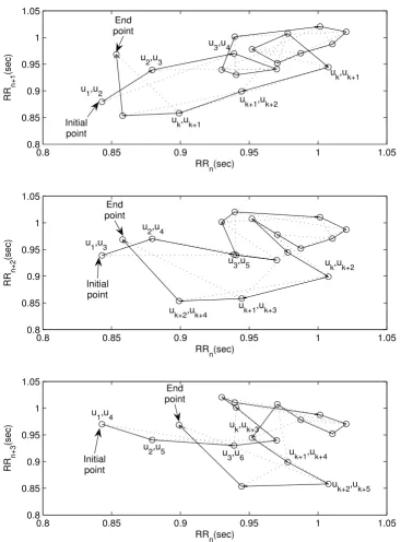
As shown in equation sets 3 and 4, for any m, the descrip-tors SD1 and SD2 only indicate m lag correlation informa-tion of the plot. This essentially conveys overall behavior of the system completely neglecting its temporal varia-tion. Figure 3 shows the Poincaré plot of RR interval time series for three different lags. From the figure, it is obvious that for any time series signal different lag plots give more insight of the signal than a single lag plot. Hence, to reflect temporal variation, we developed a descriptor to incorpo-rate multiple lag correlation information, which we call as Complex Correlation Measure (CCM). The proposed descriptor is not only related to the standard descriptors, but it also embeds temporal information, which can be used in quantification of the temporal dynamics of the system.
Methods
The development of a new descriptor, Complex Correla-tion Measure (CCM) has been presented in this secCorrela-tion. Firstly, the theoretical development has been given, fol-lowed by the analysis of the new measure with respect to the standard descriptors, SD1 and SD2. Finally, data and methodologies regarding the two case studies have been discussed which is followed by a brief description of sta-tistical analysis used in this study.
Complex Correlation Measure
In contrast to the SD1 and SD2, CCM evaluates point-to-point variation of the signal rather than gross description of the signal. Moreover, as will be seen later, CCM is a function of multiple lag correlation of the signal. The pro-posed descriptor CCM is computed in a windowed man-ner which embeds the temporal information of the signal. A moving window of three consecutive points from the
SD SDSD
RR RR
1 1
2
0 1
2= 2
=g ( )−g ( )
(1)
SD SDRR SDSD
RR
RR RR
2 2 1
2
0 1 2
2 2 2
2
= −
=g ( )+g ( )−
(2)
RR
SD m
SD F m
RR RR
RR RR
1 0
1 0
2= −
⇒ =
g g
g g
( ) ( )
( ( ), ( )) (3)
SD m RR
SD F m
RR RR
RR RR
2 0 2
2 0
2 = + − 2
⇒ =
g g
g g
( ) ( )
( ( ), ( ))
Poincaré plot are considered and the area of the triangle formed by these three points are computed. This area measures the temporal variation of the points in the win-dow. If three points are aligned on a line then the area is zero, which represents the linear alignment of the points. Moreover, since the individual measure involves three points of the two dimensional plot, it is comprised of at least four different points of the time series for lag m = 1 and at most six points in case of lag m ≥ 3. Hence the measure conveys information about four different lag
cor-relation of the signal. Now, suppose the ith window is
comprised of points a(x1, y1), b(x2, y2) and c(x3, y3) then the area of the triangle (A) for ith window can be
com-puted using the following determinant:
where A is defined on the real line ℜ and A i
x y
x y
x y
( )=1 2
1 1 1
2 2 1
3 3 1
(5) Underlying temporal dynamics of a Poincaré plot
Figure 2
Underlying temporal dynamics of a Poincaré plot. Poincaré plots with similar SD1 and SD2 values with different tempo-ral structure are shown. Top panel (A and B) shows the Poincaré plots (lag-m = 2) of two different RR intervals series of length N (N = 1000) with SD1 (0.0424 and 0.0425) and SD2 (0.1185 and 0.1185) values. The underlying temporal dynamics of first 20 points of the same RR intervals are shown in the bottom panel (C and D), which shows the visible difference among them.
0.6 0.7 0.8 0.9 1 1.1 1.2 0.6
0.7 0.8 0.9 1 1.1
RR
n+m
A
0.6 0.7 0.8 0.9 1 1.1 1.2 0.6
0.7 0.8 0.9 1 1.1
B
0.75 0.8 0.85 0.9 0.95 1 1.05 0.75
0.8 0.85 0.9 0.95 1 1.05
RRn
RR
n+m
C
0.75 0.8 0.85 0.9 0.95 1 1.05 0.75
0.8 0.85 0.9 0.95 1 1.05
RRn D SD1=0.0424
SD2=0.1185
Forming triangles in calculating CCM
Figure 3
Forming triangles in calculating CCM. Poincaré plot of RR interval time series for three different lags (m = {1, 2, 3}) are shown. It is obvious that for RR intervals with different lag plots give more insight of the signal than a single lag. Figure also shows formation of triangles by dotted lines connecting three consecutive points at different lags (m = {1, 2, 3}) for 20 RR intervals for calculating CCM. Sequence of points (RRn, RRn+m) are plotted, where RR ≡ {u1, u2, ..., uN}.
0.8 0.85 0.9 0.95 1 1.05
0.8 0.85 0.9 0.95 1 1.05
RR
n(sec)
RR
n+1
(sec)
0.8 0.85 0.9 0.95 1 1.05
0.8 0.85 0.9 0.95 1 1.05
RR
n(sec)
RR
n+2
(sec)
0.8 0.85 0.9 0.95 1 1.05
0.8 0.85 0.9 0.95 1 1.05
RR
n(sec)
RR
n+3
(sec)
u
1,u2
u
2,u3
u
3,u4
u
k,uk+1
u
k+1,uk+2
u
k,uk+1
Initial point
End point
u
1,u3
u
2,u4
u
3,u5 uk,uk+2
u
k+1,uk+3
u
k+2,uk+4
Initial point
End point
u
1,u4
u
2,u5 u
3,u6
u
k,uk+3
u
k+1,uk+4
u
k+2,uk+5
Initial point
If Poincaré plot is composed of N points then the tempo-ral variation of the plot, termed as CCM, is composed of all overlapping three point windows and can be calcu-lated as:
where m represents lag of Poincaré plot and Cn is the nor-malizing constant which is defined as, Cn = π* SD1 * SD2, represents the area of the fitted ellipse over Poincaré plot. The length of major and minor axis of the ellipse are 2*SD1, 2*SD2, where SD1, SD2 are the dispersion per-pendicular to the line of identity (minor axis) and along the line of identity (major axis) respectively.
Let the RR time series be composed of N RR interval values and defined as RR ≡u1, u2, .., uN. As shown in figure 3, the lag-1 Poincaré plot consists of N - 1 numbers of 2-D set of points PP ∈ {ℜ, ℜ} can be represented by: PP ≡ {(u1, u2),
(u2, u3), .., (uN-1, uN)} and similarly for lag of m, N - m numbers of 2-D points are expressed as:
Hence for lag-m Poincaré plot, the 1st window will be composed of points {(u1, u1+m), (u2, u2+m), (u3, u3+m)} and from equation 5, the area A can be calculated as:
Similarly the 2nd and (N - m - 2)th window is composed of
points {(u2, u2+m), (u3, u3+m), (u4, u4+m)} and {(uN-m-2, uN -2), (uN-m-1, uN-1), (uN-m, uN)} respectively. Hence the area,
A, for 2nd and (N - m - 2)th window can be calculated as:
Using equations 7, 8, 9 and 10, CCM(m) is calculated as follows:
Since RR intervals are discrete signal, the autocorrelation at lag m = j can be calculated as:
Using equations 3, 4, 11 and 12, CCM(m) can now be expressed as a function of autocorrelation at different lags. Hence,
In the above equation CCM(m) represents the point-to-point variation of the Poincaré plot with lag m as a func-tion of autocorrelafunc-tion of lags 0, m - 2, m - 1, m + 1 and m + 2. This supports our hypothesis that CCM is measured using multiple lag correlation of the signal rather than sin-gle lag. For the conventional lag-1 Poincaré plot CCM(1) can be represented as:
Analysis of Complex Correlation Measure(CCM)
In the previous section, we have given the mathematical definition of CCM and have clearly shown that CCM con-tains multiple lag correlation information of the signal. In this section, we explore the different properties of CCM with synthetic RR interval data. In our study, we used 4000 RR intervals of a synthetic RR interval (rr02) time series data from open access Physionet database [16] and the signal was divided into 20 windows with 200 RR inter-vals in each window.
Sensitivity to changes in temporal structure
Literally, the sensitivity is defined as the rate of change of the value due to the change in temporal structure of the signal. The change in temporal structure of the signal in a window is achieved by surrogating the signal (i.e, data points) in that window. In order to validate our assump-tion we calculated SD1, SD2 and CCM of a RR interval sig-nal by randomly surrogating points of each window at a time.
Now the sensitivity of descriptors ΔSD1j, ΔSD2j and
ΔCCMj were calculated using equations 14–16:
A i( ) , ,
= >
0 0
if points a, b and c are on a straight line
counnter clock-wise orientation the points a, b and c cloc
< 0, kk-wise orientation of the points a, b and c
(6)
CCM m
Cn N i A i
N ( ) ( ) || ( ) || = − = −
∑
1 2 1 2 (7)PP ≡{(u u1, 1+m),(u u2, 2+m),…,(uN m− ,uN)}
A( )1 1[u u m u u m u u m u u m u u m u u m]
2 1 2 1 3 3 1 2 1 2 3 3 2
= + − + + + − + + + − +
(8)
A u u u u u u u u
u u u u
m m m m
m m
( ) [
]
2 1
2 2 3 2 4 4 2 3 2
3 4 4 3
= − + −
+ −
+ + + +
+ +
(9)
A N m u u u u u u
u u u
N m N N m N N m N
N m N N m
( − − )= [ − +
− +
− − − − − − −
− − − − −
2 1
2 2 1 2 2
1 2 1uuN −uN m N− u −1]
(10)
CCM m
Cn N uN m Nu u u m uN m Nu u u m i u ui i m
( )
( )[
=
− − − + + − − − − + + − +
1
2 2 1 2 1 1 1 2 2
== − − + + + + + = − − = − − =
∑
∑
∑
− + − 31 1 2
1 2 1 1 2 2 2 N m
i i m i i m i i m
i N m i N m i N
u u u u u u
−−
∑
m]
(11)
gRR n n j n
N
j RR RR
( )= +
=
∑
1 (12)CCM m( )=F[gRR( ),0 gRR(m−2),gRR(m−1),gRR(m+1),gRR(m+2)]
where SD10 (= 0.36), SD20 (= 0.08) and CCM0 (= 0.16) were the parameters measured for the original data set without surrogation and j represents the window number whose data was surrogated. Moreover, SD1j, SD2j and CCMj represents the SD1, SD2 and CCM values respec-tively after surrogation of jth window. Since we divided the
entire signal in 20 windows, it resulted in 20 values of SD1, SD2 and CCM.
Sensitivity to various lags of Poincaré plot
To verify the sensitivity of SD1, SD2 and CCM with vari-ous lags of Poincaré plot, values of all descriptors were cal-culated for different time delays or lags (m was varied from 1 to 100). At each step, lag-m Poincaré plot was con-structed for the synthetic RR interval series and then SD1, SD2 and CCM values were calculated for the plot. As m was varied from 1 to 100, it resulted in 100 values of SD1, SD2 and CCM.
Case Studies
In order to validate the proposed measure – CCM, two case studies were conducted on RR interval data. The data from MIT-BIH Physionet database are [17] used in the experiments. Medical fraternity has utilized Poincaré plot, using both qualitative and quantitative approaches, for detecting and monitoring arrhythmia. Compared to arrhythmia, fewer attempts are made to utilize Poincaré plot to evaluate CHF. In this study, we have analyzed the performance of CCM and compared it with that of SD1 and SD2 for recognizing both arrhythmia and congestive heart failure using HRV signal.
HRV study of Arrhythmia and Normal Sinus Rhythm
In this study, we have used 54 long-term ECG recordings of subjects in normal sinus rhythm (30 men, aged 28.5 to 76, and 24 women, aged 58 to 73) from Physionet Nor-mal Sinus Rhythm database [17].
Furthermore, we have also used NHLBI sponsored Car-diac Arrhythmia Suppression Trial (CAST) RR-Interval Sub-study database for the arrhythmia data set from Phy-sionet. Subjects of CAST database had an acute myocar-dial infarction (MI) within the preceding 2 years and 6 or more ventricular premature complexes (PVCs) per hour
during a pre-treatment (qualifying) long-term ECG (Hol-ter) recording. Those subjects enrolled within 90 days of the index MI were required to have left ventricular ejection fractions less than or equal to 55%, while those enrolled after this 90 day window were required to have an ejection fraction less than or equal to 40%.
The database is divided into three different study groups among which we have used the Encainide (e) group data sets for our study. From that group we have chosen 272 subjects belong to subgroup baseline (no medication). The original long term ECG recordings were digitized at 128 Hz, and the beat annotations were obtained by auto-mated analysis with manual review and correction [17]. lag-1 Poincaré plots were constructed for both normal and arrhythmia subjects and the new measure CCM was com-puted along with SD1 and SD2. The SD1 and SD2 were calculated to characterize the distribution of the plots whereas CCM were used for characterizing the temporal structure of the plots.
HRV study of Congestive Heart Failure(CHF) and Normal Sinus Rhythm
For this case study, we have used 29 long-term ECG recordings of subjects (aged 34 to 79) with CHF (NYHA classes I, II and III) from Physionet Congestive Heart Fail-ure database along with 54 ECG recordings of subjects with normal sinus rhythm as discussed earlier [17]. Same ECG acquisition with beat annotations were used as dis-cussed in previous case study. Similar to previous case study, lag-1 Poincaré plots were constructed for both nor-mal and CHF subjects and the new descriptor CCM was computed as per traditional descriptors.
Statistical Analysis
In this study we have used ANOVA analysis assuming unknown and different variance for testing the hypothesis regarding mean i.e., the mean of NSR and Arrhythmia groups are equal. It suits our case studies as the sample size is small. The same test has been used to test the hypothesis for NSR and CHF group.
Results
Sensitivity to changes in temporal structure
From the mathematical definition of CCM, we anticipated that CCM would be more sensitive to changes in temporal structure within the signal than the standard descriptors. In this study, the sensitivity is defined as the rate of change of the value due to the change in temporal structure of the signal. As shown in figure 4, value of ΔCCM is much higher than ΔSD1 and ΔSD2 which indicates that CCM is much more sensitive than SD1 and SD2 to changes in underlying temporal structure of the data. This supports the mathematical definition of CCM as a sensitive meas-ure of temporal variation of the signal.
ΔSD SD j SD
SD
j
1 1 10
10
= − (14)
ΔSD SD j SD
SD
j
2 2 20
20
= − (15)
ΔCCM CCM j CCM
CCM
j=
− 0
0
Sensitivity to various lags of Poincaré plot
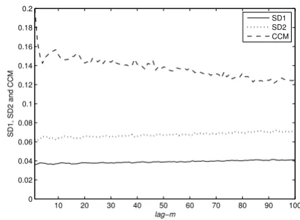
In figure 5, the relationship of CCM, SD1 and SD2 with different time delays or lags (m was varied from 1 to 100) are shown. Usually unit lag is used to create the Poincaré plot which confirms the maximum linear correlation among data points. Moreover, this lag selection may have obscured the low level nonlinearities of the signal and as a result CCM may be unable to show better performance over standard poincaré descriptors. In contrast, at higher lags, the standard descriptors are unable to capture the system dynamics. It is also established in the literature that studying behavior of descriptors as a function of lags is more informative [12]. In our study, we have found that over different lags, CCM shows more variability than SD1 and SD2. Among the three descriptors the change in val-ues for CCM was higher than both SD1 and SD2 which again supports our claim of sensitivity of CCM with signal dynamics. Hence, we conclude that the change in under-lying temporal structure due to lag of the Poincaré plot has better impact on CCM than the traditional descrip-tors.
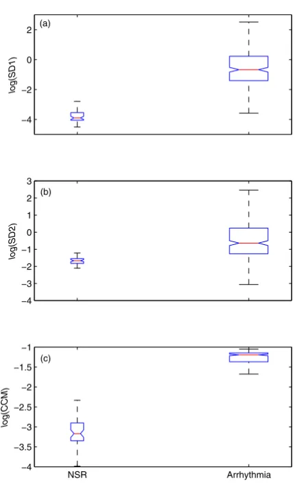
HRV studies of Arrhythmia and Normal Sinus Rhythm Figure 6 shows the box-whiskers (BW) plot of all descrip-tors for normal and arrhythmia subjects. For plotting pur-pose, log value of all descriptors are used for BW plot. Figure 6a, represents BW plot for log(SD1) and it is obvi-ous that boxes (interquartile range) of normal and arrhythmia subjects are non-overlapping. But the
whisk-ers (upper quartile) of normal subjects completely over-laps with the whiskers (lower quartile) of the arrhythmia subjects. In figure 6b, the BW plot of log(SD2) is shown and it is apparent that the BW of normal subjects com-pletely overlapped with the whiskers (lower quartile) of the arrhythmia subjects. But the box of arrhythmia sub-jects is still non-overlapping with the whiskers (upper quartile) of the normal subjects. In figure 6c, the BW plot of log(CCM) is shown and it is obvious that both of them are non-overlapping and distinct.
The p value obtained from ANOVA analysis between two groups for SD1, SD2 and CCM are given in table 1. Using ANOVA, for CCM, p = 6.28 × 10⁻¹⁸ is obtained whereas for
SD1 and SD2, it is 7.6 × 10⁻³ and 8.5 × 10⁻³ respectively. In
case of p < 0.001 to be considered as significant, only CCM would show the significant difference between two groups which indicates that CCM is a better descriptor of HRV sig-nal than SD1 and SD2 when comparing arrhythmia with normal sinus rhythm subjects.
HRV studies of Congestive Heart Failure(CHF) and Normal Sinus Rhythm
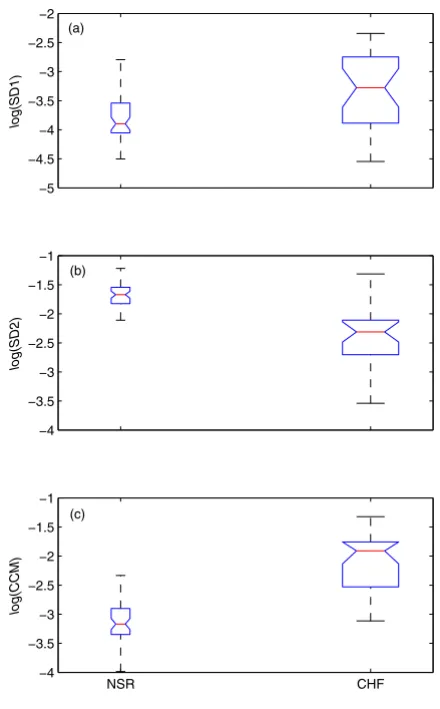
The box-whiskers plot of all descriptors for normal and CHF subjects are shown in Figure 7. Figure 7a, represents BW plot for log(SD1) and it is apparent that boxes (inter-quartile range) of normal and CHF subjects are overlap-ping. The BW of normal subjects is completely overlapped with the box and whisker (lower quartile) of the CHF sub-jects. In figure 7b, the box-whiskers plot of log(SD2) is shown and boxes are apparently non-overlapped. But the Sensitivity of descriptors with changed temporal structure
Figure 4
Sensitivity of descriptors with changed temporal structure. Sensitivity of all descriptors with change in tem-poral structure is shown. ΔSD1, ΔSD2 and ΔCCM are calcu-lated using equations 14–16. Value of ΔCCM is much higher than ΔSD1 and ΔSD2 which indicates that CCM is much more sensitive than SD1 and SD2 to the changes in underlying tem-poral structure of the data.
2 4 6 8 10 12 14 16 18 20
−0.2 0 0.2 0.4 0.6 0.8 1 1.2 1.4 1.6
Window j
Δ
SD1
j
,
Δ
SD2
j
and
Δ
CCM
j
ΔSD1 j ΔSD2 j ΔCCMj
Relationship of descriptors with different lag
Figure 5
Relationship of descriptors with different lag. Relation-ship of descriptors with different time delays or lags (m = 1 to 100) are shown. Values of SD1, SD2 and CCM were calcu-lated for different lag-m of Poincaré plot with same number of data points (N = 4000). It is found that over different lags, CCM shows more variability than SD1 and SD2.
10 20 30 40 50 60 70 80 90 100
0 0.02 0.04 0.06 0.08 0.1 0.12 0.14 0.16 0.18 0.2
lag−m
SD1, SD2 and CCM
BW plot of normal subjects mostly overlaps with the whisker (upper quartile) of the CHF subjects. In figure 7c, the BW plot of log(CCM) is shown to be non-overlapping and only the upper quartile (box) and whisker of normal
subjects are overlapped with the whisker (lower quartile) of the CHF subjects.
The values of the mean and the standard deviation for both types of subjects are shown in table 2. Last row
rep-resents the p value obtained from ANOVA analysis
between the two groups for SD1, SD2 and CCM. Though SD2 and CCM show similar difference between the mean of two subject groups, the standard deviation of CCM is lower which concentrates with the distribution of CCM values around mean comparing with that of SD2. The p value, obtained from ANOVA analysis for CCM (p = 9.07 × 10⁻¹⁴) shows more significant than SD1 and SD2.
Discussion
The main motivation for using Poincaré plot is to visual-ize the variability of any time series signal. In addition to this qualitative approach, we propose a novel quantitative measure, CCM, to extract underlying temporal dynamics in a Poincaré plot. Surrogate analysis showed that the standard quantitative descriptors SD1 and SD2 were not as significantly altered as did CCM, this is shown in figure 4. Both SD1 and SD2 are second order statistical measures [2], which are used to quantify the dispersion of the signal perpendicular and along the line of identity respectively. Moreover, SD1 and SD2 are functions of lag - m correla-tion of the signal for any m lag Poincaré plot. In contrast, CCM is a function of multiple lag (m - 2, m - 1, m, m + 1, m + 2) correlations and hence, this measure was found to be sensitive to changes in temporal structure of the signal as shown in figure 4.
From the theoretical definition of CCM it is obvious that the correlation information measured in SD1 and SD2 is already present in CCM. But this does not mean that, CCM is a derived measure from existing descriptors SD1 and SD2. Rather, CCM can be considered as an additional measure incorporating information obtained in SD1 and SD2 (as the lag m correlation is also included in CCM Distribution of descriptor values for NSR and Arrhythmia
subjects
Figure 6
Distribution of descriptor values for NSR and Arrhythmia subjects. The distribution of descriptors are shown using Box-whiskers (BW) plot (without outliers) of (a) log(SD1), (b) log(SD2) and (c) log(CCM) for Normal Sinus Rhythm (NSR, n = 54) and Arrhythmia (n = 272) subjects. From panel a, it is obvious that boxes (interquartile range) of normal and arrhythmia subjects are non-overlapping. But the whiskers (upper quartile) of normal subjects completely overlaps with the whiskers (lower quartile) of the arrhythmia subjects. From panel b, it is apparent that the BW of normal subjects completely overlapped with the whiskers (lower quartile) of the arrhythmia subjects. But the box of arrhyth-mia subjects is still non-overlapping with the whiskers (upper quartile) of the normal subjects. From panel c, it is obvious that both of them are non-overlapping and distinct.
−4 −2 0 2
log(SD1)
−4 −3 −2 −1 0 1 2 3
log(SD2)
NSR Arrhythmia −4
−3.5 −3 −2.5 −2 −1.5 −1
log(CCM)
(a)
(b)
(c)
Table 1: Mean ± Standard deviation of all descriptors with p values for NSR and Arrhythmia subjects
SD1 SD2 CCM
NSR 0.03 ± 0.02 0.19 ± 0.04 0.05 ± 0.03 Arrhythmia 1.92 ± 5.18 2.30 ± 5.86 0.26 ± 0.08
p value (ANOVA) 7.60E-3 8.50E-3 6.28E-18
measure). In a Poincaré plot, it is expected that lag response is stronger at lower values of m and it attenuates with increasing values of m. This is due to the dependence of Poincaré descriptors on autocorrelation functions. The autocorrelation function monotonically decreases with increasing lags and in case of RR interval time series, usu-ally the current beat influences only about six to eight suc-cessive beats [12]. In our study, we also found that all measured descriptors SD1, SD2 and CCM changed rapidly at lower lags and the values are stabilized with higher lag values (figure 5). Since, CCM is also a function of signals autocorrelations, it shows a similar lag response to that shown by SD1 and SD2. Therefore, CCM may be used to study the lag response behavior of any pathological con-dition in comparison with normal subjects, or controls.
HRV measure is considered to be a better marker for increased risk of arrhythmic events than any other nonin-vasive measure [18,19]. An earlier study has shown that Poincaré plots exposed completely different 2D patterns in the case of arrhythmia subjects [20]. These abnormal medical conditions have complex patterns due to reduced autocorrelation of the RR intervals. Consequently due to the changes in autocorrelation, we have found that the variability measure using Poincaré (SD1, SD2) was higher than normal subjects (shown in table 1). Moreover, the fluctuations of these variability measures were also very high in the case of arrhythmias. This may be due to differ-ent types of arrhythmia along with subjective variation of HRV. In arrhythmia subjects, CCM was found to be higher compared to NSR subjects, but the deviation due to sub-jective variation is much smaller than SD1 and SD2. As a result, CCM linearly separates these two groups of subjects which means that the effect of different types of arrhyth-mia and subjective variation are reduced while using CCM than other variability measures. Therefore, we may con-clude that CCM is a better marker for recognizing arrhyth-Distribution of descriptor values for NSR and CHF subjects
Figure 7
Distribution of descriptor values for NSR and CHF subjects. The distribution of descriptors are shown using Box-whiskers (BW) plot (without outliers) of (a) log(SD1), (b) log(SD2) and (c) log(CCM) for Normal Sinus Rhythm (NSR, n = 54) and Congestive Heart Failure (CHF, n = 29) subjects. From panel a, it is apparent that boxes (interquar-tile range) of normal and CHF subjects are overlapping. The BW of normal subjects is completely overlapped with the box and whisker (lower quartile) of the CHF subjects. In panel b, boxes are apparently non-overlapped. But the BW plot of normal subjects mostly overlaps with the whisker (upper quartile) of the CHF subjects. In panel c, the BW plot of log(CCM) is shown to be non-overlapping and only the upper quartile (box) and whisker of normal subjects are overlapped with the whisker (lower quartile) of the CHF subjects.
−5 −4.5 −4 −3.5 −3 −2.5 −2
log(SD1)
−4 −3.5 −3 −2.5 −2 −1.5 −1
log(SD2)
NSR CHF
−4 −3.5 −3 −2.5 −2 −1.5 −1
log(CCM)
(a)
(b)
(c)
Table 2: Mean ± Standard deviation of all descriptors with p values for NSR and CHF subjects.
SD1 SD2 CCM
NSR 0.03 ± 0.02 0.19 ± 0.04 0.05 ± 0.03 CHF 0.04 ± 0.02 0.11 ± 0.06 0.14 ± 0.06
p value (ANOVA) 5.65E-4 5.04E-12 9.07E-14
mia than the traditional variability measures of Poincaré plot.
In another case study, we have shown as to how Poincaré plot can be used to characterize CHF subjects from normal subjects using RR interval time series. Compared to SD2, SD1 and CCM values were found to be higher in CHF sub-jects. This findings might indicate that the short term var-iation in HRV is higher in CHF subjects, however, the long term variation is reduced. Since CCM captures the signal dynamics at short level (i.e, 3 points of the plot), it appears to be affected by short term variation of the signal in CHF subjects. In the case of recognition of CHF sub-jects, although SD2 showed good result CCM was found to be more significant as shown in table 2.
Above discussion indicates that CCM is an additional descriptor of Poincaré plot with SD1 and SD2. This also implies that CCM is a more consistent descriptor com-pared to SD1 and SD2. Considering the presented case studies, it is clear that neither SD1 nor SD2 alone can independently distinguish between normal and pathol-ogy. However, in the same scenario, CCM has the ability to perform the classification task independently. This jus-tifies the usefulness of the proposed descriptors as a fea-ture in a pattern recognition scenario. Our primary motivation for detecting pathology with a novel descrip-tor like CCM rather than by observing visual pattern is achieved as shown by the case studies described. In this study, we have not looked at the physiological interpreta-tion of CCM which remain to be studied in future. How-ever, a few remarks on this would be appropriate. The Poincaré plot reflects the autocorrelation structure through the visual pattern of the plot. The standard descriptors SD1 and SD2 summarizes these correlation structure of RR interval data as shown by Brennan et. al. [2]. CCM is based on the autocorrelation at different lags of the time series hence giving an in-depth measurement of the correlation structure of the plot. Therefore, the value of CCM decreases with increased autocorrelation of the plot. In arrhythmia, the pattern of the Poincaré plots becomes more complex [20] and thus reducing the corre-lation of the signal (RRi, RRi+1). In case of healthy subjects the value of CCM is lower than that of arrhythmic sub-jects. In future, it might be worth looking at the perform-ance of CCM for other pathologies.
Conclusion
The proposed Complex Correlation Measure is based on the limitation of standard descriptors SD1 and SD2. The analysis carried out confirms the hypothesis that CCM measures the temporal variation of the Poincaré plot. In contrast to the standard descriptors, CCM evaluates point-to-point variation of the signal rather than gross variabil-ity of the signal. We have shown that CCM is more
sensi-tive to changes in temporal variation of the signal. We have further demonstrated that CCM varies with different lags of Poincaré plot. Besides the mathematical definition of CCM and analyzing properties of the measure, we have also evaluated the performance of CCM using real world case studies. CCM was found to be effective in the assess-ment of both arrhythmia and CHF against normal sinus rhythm. In future, CCM may be used as an efficient feature for pathology detection.
Competing interests
The authors declare that they have no competing interests.
Authors' contributions
CKK conceived, derived and implemented the new descriptor, collected the data and wrote the manuscript with supervision of AHK and MP. AHK, JG and MP con-tributed to the development of the new descriptor and participated in the discussion and interpretation of the results. In addition, AHK contributed to revision of the manuscript. All authors read and approved the final man-uscript.
Acknowledgements
Dr. Mak Adam Daulatzai read the manuscript and made improvement.
References
1. Tulppo MP, Makikallio TH, Takala TES, Seppanen T, V HH: Quanti-tative beat-to-beat analysis of heart rate dynamics during exercise. Am J Physiol 1996, 271:H244-H252.
2. Brennan M, Palaniswami M, Kamen P: Do existing measures of poincare plot geometry reflect nonlinear features of heart rate variability. IEEE Trans on Biomed Engg 2001, 48:1342-1347. 3. Liebovitch LS, Scheurle D: Two lessons from fractals and chaos.
Complexity 2000, 5:34-43.
4. Acharya UR, Joseph KP, Kannathal N, Lim CM, Suri JS: Heart rate variability: a review. Medical and Biological Engineering and Comput-ing 2006, 44(12):1031-1051.
5. Tulppo MP, Makikallio TH, Seppanen T, Airaksinen JKE, V HH: Heart rate dynamics during accentuated sympathovagal interac-tion. Am J Physiol 1998, 247:H810-H816.
6. Toichi M, Sugiura T, Murai T, Sengoku A: A new method of assess-ing cardiac autonomic function and its comparison with spectral analysis and coefficient of variation of R-R interval. J Auton Nerv Syst 1997, 62:79-84.
7. Hayano J, Takahashi H, Toriyama T, Mukai S, Okada A, Sakata S, Yamada A, Ohte N, Kawahara H: Prognostic value of heart rate variability during long-term follow-up in chronic haemodial-ysis patiens with end-stage renal disease. Nephrol Dial Trans-plant 1999, 14:1480-1488.
8. Casolo G, Bali E, Taddei T, Amuhasi J, Gori C: Decreased sponta-neous heart rate variability in congestive heart failure. Am J Cardiol 1989, 64(18):1162-1167.
9. Woo MA, Stevenson WG, Moser DK, Trelease RB, Harper RM: Pat-terns of beat-to-beat heart rate variability in advanced heart failure. Am Heart J 1992, 123(3):704-710.
10. Thuraisingham RA: Enhancing Poincare plot information via sampling rates. Applied Mathematics and Computation 2007, 186:1374-1378.
11. Lerma C, Infante O, Perez-Grovas H, Jose MV: Poincare plot indexes of heart rate variability capture dynamic adapta-tions after haemodialysis in chronic renal failure patients. Clin Physiol Funct Imaging 2003, 23(2):72-80.
Publish with BioMed Central and every scientist can read your work free of charge
"BioMed Central will be the most significant development for disseminating the results of biomedical researc h in our lifetime."
Sir Paul Nurse, Cancer Research UK
Your research papers will be:
available free of charge to the entire biomedical community
peer reviewed and published immediately upon acceptance
cited in PubMed and archived on PubMed Central
yours — you keep the copyright
Submit your manuscript here:
http://www.biomedcentral.com/info/publishing_adv.asp
BioMedcentral 13. Negro CAD, Wilson CG, Butera RJ, Rigatto H, Smith JC:
Periodic-ity, Mixed-Mode Oscillations, and Quasiperiodicityin a Rhythm-Generating Neural Network. Biophysical Journal 2002, 82:206-214.
14. Schechtman VL, Lee MY, Wilson AJ, Harper RM: Dynamics of res-piratory patterning in normal infants and infants who subse-quently died of the sudden infant death syndrome. Pediatric Research 1996, 40:571-577.
15. Brennan M, Palaniswami M, Kamen P: Poicare plot interpretation using a physiological model of HRV based on a network of oscillators. Am J Physiol Heart Circ Physiol 2002, 283:1873-1886. 16. Website TP: Computers in Cardiology Challenge 2002 (CinC
2002): RR Interval Time Series Modelling. 2002 [http:// www.physionet.org/challenge/2002/].
17. Goldberger AL, Amaral LA, Glass L, Hausdorff JM, Ivanov PC, Mark RG, Mietus JE, Moody GB, Peng CK, Stanley HE: PhysioBank, Phys-ioToolkit, and PhysioNet: Components of a New Research Resource for Complex Physiologic Signals. Circulation 2000, 101(23):e215-e220.
18. Eisenberg MJ: Risk stratification for arrhythmic events: are the bangs worth the bucks? J Am Coll Cardiol 2001, 38(71912-1915 [http://content.onlinejacc.org].
19. Hartikainen JE, Malik M, Staunton A, Poloniecki J, Camm AJ: Distinc-tion between arrhythmic and nonarrhythmic death after acute myocardial infarction based on hear rate variability, signal-averaged electrocardiogram, ventricular arrhythmias and left ventricular ejection fraction. J Am Coll Cariol 1996, 28(2):296-304.