Mikkel N. Schmidt [email protected]
University of Cambridge, Department of Engineering, Trumpington Street, Cambridge, CB2 1PZ, UK
Abstract
We introduce a new approach to non-linear regression called function factorization, that is suitable for problems where an output vari-able can reasonably be modeled by a num-ber of multiplicative interaction terms be-tween non-linear functions of the inputs. The idea is to approximate a complicated func-tion on a high-dimensional space by the sum of products of simpler functions on lower-dimensional subspaces. Function factoriza-tion can be seen as a generalizafactoriza-tion of matrix and tensor factorization methods, in which the data are approximated by the sum of outer products of vectors. We present a non-parametric Bayesian approach to function factorization where the priors over the fac-torizing functions are warped Gaussian pro-cesses, and we do inference using Hamilto-nian Markov chain Monte Carlo. We demon-strate the superior predictive performance of the method on a food science data set com-pared to Gaussian process regression and ten-sor factorization using PARAFAC and GE-MANOVA models.
1. Introduction
In many regression problems, the output variable can only be reasonably explained by interactions between the input variables. An example, which we shall return to in our experiments, is measurements of the color of meat under different storage conditions. Color is an important quality that affects the consumers choice, and it is thus important to understand and model how the color is influenced by different explanatory factors such as storage time, temperature, oxygen content in the atmosphere, and exposure to light. It is reasonable to assume, that the color of meat does not vary
lin-Appearing inProceedings of the 26thInternational Confer-ence on Machine Learning, Montreal, Canada, 2009. Copy-right 2009 by the author(s)/owner(s).
early with each of the explanatory variables, but that it depends on interactions of the explanatory variables in a non-linear fashion.
In this paper we present a new approach to non-linear regression that is suitable for problems where the out-put variable can be reasonably explained by non-linear interactions of the inputs. The goal in regression anal-ysis is to infer a mapping function, y:X →R, based onNobserved input-output pairs,D={(xn, yn)}N
n=1,
wherexn ∈ X are inputs andyn∈Rare outputs. The
Bayesian approach to the regression problem is to for-mulate a prior distribution over mapping functions and combine this with the data using a suitable observa-tion model to infer the posterior distribuobserva-tion over the mapping function. The posterior can then, for exam-ple, be used to make inference about the value of the output, y∗, at a previously unseen position in input
space, x∗, by computing the predictive distribution
which involves integrating over the posterior.
The main idea in function factorization is to ap-proximate a complicated function, y(x), on a
high-dimensional space, X, by the sum of products of a number of simpler functions,fi,k(xi), on lower
dimen-sional subspaces,Xi, y(x)≈ K X k=1 I Y i=1 fi,k(xi). (1)
We refer to this as a K-component I-factor function factorization model.
In the model, we assume that the inputs,xn∈ X, can
naturally be divided intoIinputs that lie in subspaces of X, x1
n ∈ X 1
, . . . ,xI
n ∈ XI, and that the output
is reasonably modeled by a number of multiplicative interaction terms between non-linear functions of the inputs. The subspaces need not be chosen to be dis-joint; for example, two subspaces could be identical which makes it possible for the model to capture non-stationary modulation effects.
Bayesian inference in function factorization models re-quires the specification of a likelihood function as well as priors over the factorizing functions. These priors
could for example be chosen by selecting a suitably flexible parameterized family of functions and assume prior distributions over the parameters. Another ap-proach, which we will pursue in this paper, is to as-sume a non-parametric distribution over the functions. Specifically, we choose warped Gaussian process pri-ors.
2. Relation to other methods
Function factorization with warped Gaussian process priors (FF-WGP) generalizes a number of other well known machine learning techniques including matrix and tensor factorization, linear regression, and warped Gaussian process regression. In the following, we give an overview of the relation to these methods.
2.1. Relation to matrix and tensor factorization
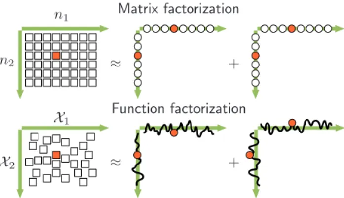
Function factorization generalizes matrix and tensor factorization models, as illustrated in Figure 1. In ma-trix factorization, a data mama-trix, Y, is approximated
by the product of two matrices,F1andF2,
Y ≈F⊤1F2. (2)
To make the relation to function factorization explicit, we can rewrite this as
yn1,n2 ≈ K X k=1 2 Y i=1 fi,k ni , (3)
where yn1,n2 is element (n1, n2) ofY and fni,k is
ele-ment (k, n) of Fi. Comparing this with Eq. (1), we
note that the main difference between matrix factor-ization and function factorfactor-ization is that in the former the goal is to learn a set of parameters, fi,k
ni, whereas
in the latter a set of functions,fi,k(xi), are learned.
In matrix factorization data points lie on a regular grid in the joint space of column and row indices, (n1, n2), and are approximated by the sum of outer products of two factors, which are vectors defined on the column and row indices respectively. In function factorization, data points lie in the spaceX and are approximated by the sum of products of functions defined on subspaces ofX.
In function factorization the priors can be chosen, for example, to have support over the non-negative num-bers or to have a sub- or super-Gaussian density, which will lead to generalizations of certain Bayesian for-mulations of non-negative matrix factorization (NMF) and independent component analysis (ICA). Similar analogies exists between function factorization and
≈ ≈ + + n1 n2 X1 X2 Matrix factorization Function factorization
Figure 1.Illustration of the relation between matrix fac-torization and function facfac-torization. In matrix factoriza-tion, data lie on a regular grid and is approximated by a product-sum of vectors. In function factorization, data lie inX and are approximated by a product-sum of functions over subspaces ofX.
higher-order decompositions of tensors such as the par-allel factor analysis (PARAFAC) model.
Schmidt and Laurberg’s (2008) method for non-negative matrix factorization with Gaussian process priors can be seen as aK-component two-factor func-tion factorizafunc-tion model, where the data is required to be in the form of a matrix, and inference is done by computing a maximum a posteriori estimate.
2.2. Relation to linear regression
Function factorization can also be seen as a generaliza-tion of linear regression. To show this, we start from the basic linear regression equation, where the outputs are modeled by a linear combination of the inputs,
yn≈ K X i=k xknβk, (4) where xk
n denotes the kth element of xn and βk are
regression coefficients. Since this model is linear and additive in the inputs, it does not model non-linear effects and interactions between the inputs. To over-come these issues, linear regression can be performed on non-linear interactive terms,
yn ≈ K X
k=1
fk(xin)βk, (5)
wherefkare non-linear functions of all the input
vari-ables. To show the relation to function factorization, we choose fk as a product of non-linear
transforma-tions of the inputs, yn ≈ K X k=1 I Y i=1 fi,k(xin) ! βk. (6)
This expression is very similar to Eq. (1); however, in linear regression the objective is to learn the regression coefficients,βk, for fixed non-linear transformations of
the inputs, whereas in function factorization the aim is to learn the non-linear functions themselves. Function factorization generalizes this formulation of linear re-gression, since the regression coefficients without loss of generality can be incorporated into the non-linear functions.
2.3. Relation to warped Gaussian processes
Function factorization generalizes warped Gaussian process (WGP) regression, when WGP priors are as-sumed over the factorizing functions. Obviously, when
K = I = 1, FF-WGP collapses to WGP regression; however, in models with multiple factors the two meth-ods differ in the assumptions that are made about the data.
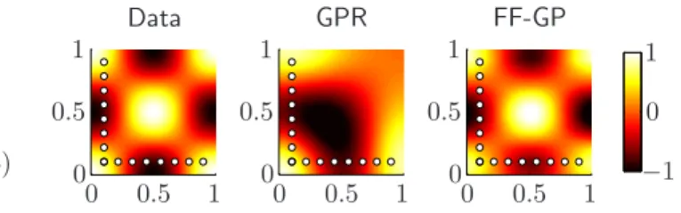
A simple illustration is given in Figure 2 for a two-dimensional toy data problem generated as the prod-uct of two cosine functions. Fifteen data points were chosen from the function and regression analysis was performed using a GP and a one-component two-factor function factorization with GP priors. In regions of the function that are far away from any of the observed in-put points, the GP tends to its zero mean prior. The function factorization method on the other hand as-sumes that the data has a multi-linear structure, and since that assumption in this case is correct, the data is modeled accurately even in regions with no obser-vations. In many data sets, the assumption that the outputs are well modeled by multiplicative interactive terms is reasonable, and when the assumptions holds, function factorization can provide better results than Gaussian process regression based methods.
Adams and Stegle’s (2008) Gaussian process prod-uct model, in which a function is modeled as the point-wise product of two Gaussian processes for the purpose of capturing non-stationarities, can be seen as a one-component two-factor function factorization model with Gaussian process priors, where the two factorizing functions are both defined over the entire space,X. −1 0 0 0 0 0 0 0 0.5 0.5 0.5 0.5 0.5 0.5 1 1 1 1 1 1 1 Data GPR FF-GP
Figure 2.A simple toy example that illustrates important differences between Gaussian process regression and func-tion factorizafunc-tion. Left: A two-dimensional toy data set is constructed as the multiplication of two cosines and 15 data points are chosen at the indicated positions. Mid-dle: Gaussian process regression on the data points fits the data well in the region close to the observation, and far away from the observations it tends to its zero mean prior. Right: A one-component function factorization on the same data fits the data well in the entire region, due to the correct assumption that the data comes from a product of two functions.
3. Function factorization using warped
Gaussian processes
In the following, we describe a non-parametric Bayesian approach to function factorization using warped Gaussian process (WGP) priors over the fac-torizing functions. First, we give a summary of the WGP, and then we describe function factorization us-ing WGP priors. Finally, we present an inference procedure based on Hamiltonian Markov chain Monte Carlo (HMCMC).
3.1. Warped Gaussian processes
A Gaussian process1
(GP) is a flexible and practical method for specifying a non-parametric distribution over a function, g(x). It is fully characterized by its
mean function, m(x) = E g(x)
, and its covariance function,c(x,x′) =E
g(x)−m(x)
g(x′)−m(x′)
. We use the notationg(x)∼ GP m(x), c(x,x′)to
de-note a random function drawn from a GP.
The GP is limited in the sense that it assumes that any finite subset of values of the functiong(x) follow
a joint multivariate Gaussian distribution. The idea behind the warped Gaussian process (WGP) (Snelson et al., 2004) is to overcome this limitation by map-ping the GP through a non-linear warp function,h(g), parameterized byθh,
y(x) =h g(x)
, g(x)∼ GP m(x), c(x,x′) , (7)
1
See Rasmussen and Williams (2006) for a comprehen-sive introduction to Gaussian processes in machine learn-ing.
x1 x2 x3 xN y1 y2 y3 yN µ1 µ2 µ3 µN g1 g2 g3 gN θh θc θy i k
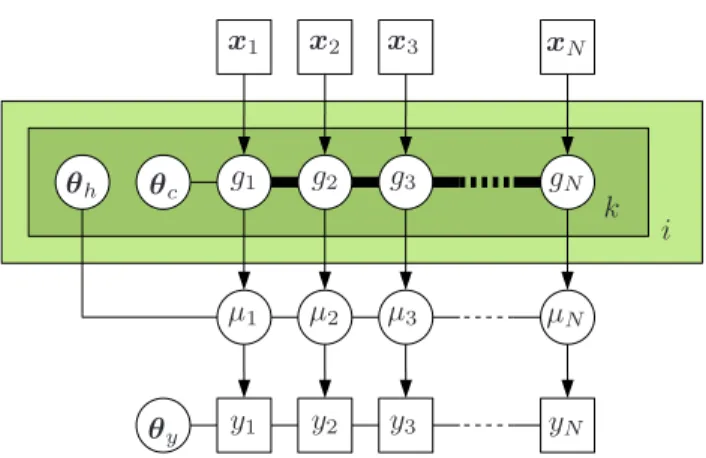
Figure 3.Graphical model for the function factorization model with warped Gaussian process priors. Squares repre-sent observed variable and circles denote unobserved vari-ables and parameters. The bold line indicates that the nodesgi,k1 , . . . , g
i,k
N are fully connected.
and jointly learn the parameters of the GP and the warp function. Snelson et al. (2004) learn the param-eters of the WGP by maximum likelihood, but they note that priors can be included to learn maximum a posteriori estimates or Markov chain Monte Carlo can be used to integrate out the parameters.
3.2. The FF-WGP model
Letµ(x) denote a function factorization model,
µ(x) = K X k=1 I Y i=1 fi,k(x), (8)
wherefi,k(x) are modeled by zero mean WGPs. In the
most general formulation, each factor in each compo-nent has distinct warp and covariance functions,
fi,k(x) =hi,k gi,k(x)
, (9)
gi,k(x)∼ GP 0, ci,k(x,x′)
. (10) We then model the outputs, yn, as independent and
identically distributed given µn =µ(xn), using some
likelihood function,p(yn|µn), parameterized byθy.
A graphical model of the FF-WGP is shown in Fig-ure 3. The unknowns in the model are the parameters of the likelihood function,θy, the warp functions,θh,
and the covariance functions,θc, as well as the latent
variables,gi,k
n =gi,k(xn). 3.3. Change of parameters
The latent variables,gi,k
n , have a multivariate Gaussian
distribution a priori, and are thus highly correlated.
We have found empirically that MCMC inference in the model is more efficient when we perform a change of variables, such that the latent variables are uncor-related a priori. We do this by defining a new latent variable,zni,k′, related togi,kn by
gi,kn = N X n′=1 Cni,k′,nz i,k n′ , (11)
where Cn,ni,k′ holds the Cholesky decomposition of the
covariance matrix of the (i, k)th Gaussian process,
N X n′′=1 Cn,ni,k′′C i,k n′,n′′=c i,k n,n′ =c i,k(x n,xn′). (12)
With this change of variables, the model can be written as µn= K X k=1 I Y i=1 hi,k N X n′=1 Cni,k′,nz i,k n′ ! , (13) and the prior over the new latent variables are i.i.d. standard Gaussian,zni,k′ ∼ N(0,1). We emphasize that
this change of variables does not change the model— only its parameterization.
3.4. Posterior and predictive distribution
The joint posterior distribution of the latent variables and the parameters conditioned on the data is given by p(z,θ|D)∝p(θ) N Y n=1 p(yn|µn) I Y i=1 K Y k=1 p(zni,k) ! , (14) where z = {zi,k
n } denotes all latent variables, θ = {θy,θh,θc}denotes all parameters, andµn is defined
in Eq. (13).
To infer the value of the output y∗ at a previously
unseen point x∗ we must evaluate the predictive
tribution, which requires integrating the posterior dis-tribution over the latent variables and parameters,
p(y∗|x∗,D) =
Z Z
p(y∗|x∗,z,θ)p(z,θ|D)dzdθ. (15)
Since this integral is analytically intractable, we ap-proximate it by Monte Carlo sampling, i.e., we draw
M samples, {zm,θm }M
m=1, from the posterior
distri-bution in Eq. (14) and approximate Eq. (15) by the sum p(y∗|x∗,D)≈ M X m=1 p(y∗|x∗,zm,θm). (16)
This expression can be directly evaluated, if the input point, x∗, coincides with at least one data point,xn,
on all subspaces, Xi, because then all required latent
variables are instantiated in the posterior sample. In the toy example in Figure 2, for example, this means that Eq. 16 can be directly evaluated on the 8-by-8 grid formed by the 15 input points. To evaluate the predictive distribution outside these points we instead draw samples from the predictive distribution.
3.5. Inference using Hamiltonian Markov chain Monte Carlo
Since we can not directly draw samples from the posterior distribution in Eq. (14), we use a Markov chain Monte Carlo sampling procedure. Hamilto-nian Markov chain Monte Carlo (HMCMC) (Duane et al., 1987) is an attractive method for this prob-lem, because it improves on the sometimes slow con-vergence rates due to the random walk behavior of other MCMC methods such as Gibbs sampling and Metropolis-Hastings. HMCMC requires the computa-tion of derivatives of the logarithm of the posterior distribution with respect to all variables and parame-ters, which can be done as we show in the following. We defineL which is proportional to the negative log posterior up to an additive constant
L= −logp(θ)− N X n=1 logp(yn|µn) − I X i=1 K X k=1 zi,k n 2 2 . (17)
We now need to compute the derivatives of L with respect to the latent variables and all parameters of the model. The derivative with respect to the latent variables requires the computation of the derivate of the log likelihood and of the warp functions,
∂L ∂zni,k′ = − N X n=1 ∂logp(yn|µn) ∂µn Y i′6=i hin′,k × ∂hi,k n ∂gni,k Cni,k′,n+z i,k n′ . (18)
The derivative with respect to the parameters of the likelihood function is straightforward, and has two terms: the derivative of the prior and the derivative of the log likelihood,
∂L ∂θy =− ∂logp(θ) ∂θy − N X n=1 ∂logp(yn|µn) ∂θy . (19)
Similarly, the derivate with respect to the parameters of the warp functions has two terms: the derivative
of the prior and the derivative of the log likelihood, where we use the chain rule,
∂L ∂θh = − ∂logp(θ) ∂θh − N X n=1 ∂logp(yn|µn) ∂µn × K X k=1 I X i=1 Y i′6=i hi′,k n ∂hi,k n ∂θh . (20)
The derivative with respect to the parameters of the covariance function is a bit more involved, since it re-quires the computation of the derivative of a Cholesky decomposition. We begin with the derivative of the log posterior with respect to the Cholesky decomposition itself ∂L ∂Cni,k′,n =∂logp(yn|µn) ∂µn Y i′6=i hi′,k n ∂hi,k n ∂gi,kn zni,k′. (21)
Using this, we can compute the backward derivative (Smith, 1995) of the Cholesky decomposition, Fn,ni,k′,
and finally the desired derivative can be evaluated as
∂L ∂θc = N X n=1 N X n′=1 Fn,ni,k′ ∂ci,kn,n′ ∂θc . (22)
The computation of the derivative of the Cholesky decomposition is approximately as computationally expensive as computing a Cholesky decomposition which is the most expensive computation in the WGP method. For that reason, the use of the backwards derivative is attractive when we need to compute the derivative with respect to several parameters of a co-variance function, since the backward derivate needs only be computed once.
4. Experiments
We evaluated the proposed model on a food science data set (Bro & Jakobsen, 2002) that consists of mea-surements of the color of fresh beef as it changes during storage under different conditions. The storage condi-tions are determined by the values of five independent variables summarized in Table 1. In a reduced facto-rial experimental design, measurements were taken at a subset of the possible combinations of values of the independent variables, such that the data can be rep-resented as a five-dimensional tensor with 60% of the values missing. A detailed description of the experi-mental design and the data is given by Bro and Jakob-sen (2002) who analyze the data using generalized mul-tiplicative analysis of variance (GEMANOVA). We note, that because of the factorial experimental de-sign, the input data points lie on a regular grid which
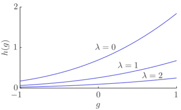
λ= 0 λ= 1 λ= 2 −01 0 1 1 2 g h ( g )
Figure 4.Warp function that transforms a standard Gaus-sian distribution into an exponential distribution with log scaleλ.
is a requirement in order to analyze the data using tensor factorization methods, suitably tailored to han-dle missing data (Tomasi & Bro, 2002). The function factorization method does not require the data to lie on a grid, and its applicability thus extends beyond multiway array data.
4.1. Model choice
In our experiments we use a Gaussian likelihood,
p(yn|µn) = 1 p 2πexp(v)exp −(yn−µn) 2 2 exp(v) , (23) parameterized by the log variance, θy = {v}, which
ensures that the variance is always positive. This like-lihood function allows us to directly compare our re-sults with those of Bro and Jakobsen (2002) who use least squares PARAFAC and GEMANOVA models to analyze the same data.
The purpose of the warp functions is to map the Gaus-sian outputs of the GPs into another desired distribu-tion. In the present data we expect the factorizing functions to be non-negative, because the output vari-able that measures the red color of the meat is inher-ently non-negative. We use a particular warp function, illustrated in Figure 4,
hi,k(g) =−exp(−λi) log
1 2 − 1 2erf g √ 2 , (24) parameterized by log scale parameters θh = {λi
}. This warp function was suggested by Schmidt and Lau-rberg (2008) and has the property that it transforms a standard Gaussian variable to an exponentially dis-tributed variable.
For the first four independent variables, shown in
Ta-ble 1, we choose a Gaussian covariance function,
ci,k(x,x′) = exp −exp(ℓi)||x−x′||2, (25)
parameterized by log length-scale parameters θc = {ℓi
}. We choose the covariance function for the fifth independent variable, the muscle number, as a delta function,
ci,k(x,x′) =δ(x−x′), (26)
such that this factor is effectively modeled as an expo-nentially distributed random variable.
For simplicity, we choose a non-informative flat (im-proper) prior over all parameters, p(θ) ∝ 1, but we
note that it is straightforward to choose proper priors over the parameters in a hierarchical fashion, and in-clude any hyper-parameters in the HMCMC inference procedure.
4.2. Cross-validation
We divided the data set into ten subsets and performed ten-fold cross-validation. We included three different FF-WGP models in our experiments: K = {1,2,3}. In each run, we ran the HMCMC sampler for 5000 it-erations using 20 leapfrog steps in each iteration and discarded the first half of the samples to allow the sampler to burn in. Plots of the samples of the pa-rameters indicated that the sampling procedure had stabilized after a few hundred iterations. As an ex-ample, the log variance parameter, v, as a function of the iteration number is shown in Figure 5 for one of the HMCMC runs. We then computed the posterior mean estimate of the held-out data. For comparison we fitted K = {1,2,3} component PARAFAC mod-els using the N-way toolbox (Andersson & Bro, 2000). We also fitted a standard Gaussian process with Gaus-sian covariance by maximum likelihood and computed the posterior mean of the held-out data. For all of the models, we then computed the root mean squared error of the held out data.
4.3. Results
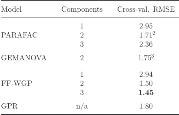
The results of the experiments are given in Table 2. A one-component PARAFAC model yielded a relatively high cross-validation error, whereas a two-component PARAFAC yields a relatively low error. A three-component PARAFAC leads to over-fitting, i.e., it fit-ted the training data better but gave a higher cross-validation error.
The two-component GEMANOVA model is suggested by (Bro & Jakobsen, 2002) as a good tradeoff between model complexity and predictive quality, and corre-sponds to a restricted PARAFAC model with some of
1000 2000 3000 4000 5000 0 0 1 2 3 v Iteration
Figure 5.Log variance parameter, v, as a function of it-eration number in one run of the HMCMC sampler for a two-component FF-WGP model.
Table 1.Independent variables that affect the color of beef as it changes during storage.
Independent variable Unit Values
Storage time Days 0,3,7,8,10
Temperature ◦C 2,5,8
Oxygen content in head-space % 40,60,80 Exposure time to light % 0,50,100
Muscle number 1,2,3,4,5,6
the factors fixed. In the experiments of Bro and Jakob-sen (2002), the GEMANOVA model yields a cross-validation error comparable to our results on a two-component PARAFAC model, but using fewer param-eters.
Our result for the one-component FF-WGP model was similar to the one-component PARAFAC, which again suggests that one multiplicative component is not enough to adequately describe the data. Two- and three-component FF-WGP models yielded better pre-dictions and had no problems with over-fitting, since all parameters are integrated out using MCMC. Gaus-sian process regression performed slightly worse than the factorization based models, possibly because the factorial structure of the problem is not exploited. Figure 6 shows the learned factor pertaining to stor-age time in the one-component PARAFAC and FF-WGP model. In the PARAFAC model, the value of the factor can only be estimated at the five input po-sitions at which data points were available. The func-tion factorizafunc-tion approach on the other hand gives a full posterior distribution over a function, which can be evaluated anywhere. The two methods agree that
1 0.9 0.8 0.7 0 2 4 6 8 10 Days FF-WGP PARAFAC
Figure 6.Relative effect of storage time: The factor per-taining to storage time in one-factor PARAFAC and FF-WGP models. The PARAFAC model estimates the value of the factor at the five points at which data was recorded. The FF-WGP outputs a posterior distribution over func-tions. The plot shows the posterior mean and standard deviation.
storage time negatively influences the color of beef in a near-linear manner.
5. Conclusions
We have presented a new approach to non-linear re-gression called function factorization. The method is based on approximating a function in a high-dimensional space as the sum of products of functions on subspaces. Using warped Gaussian processes as non-parametric priors, we have presented a Bayesian inference procedure based on Hamiltonian Markov chain Monte Carlo sampling.
Factorization based methods such as the PARAFAC model, that model data as a product of factors, can lead to intuitive and interpretable results when the factors have a physical meaning. Non-parametric Bayesian regression methods, such as the warped Gaussian process, make fewer assumptions on the structure of the data, but lack the same interpretabil-ity. The function factorization method presented here combines the idea of a factorized model with the flex-ibility of non-parametric Bayesian regression.
On a food science data set we have shown that the function factorization method using warped Gaussian process priors leads to superior performance in terms of cross-validated root mean squared error on a
pre-2
Our results differ from Bro and Jakobsen (2002) who note that the model is degenerate but report a leave-one-out cross-validation RMSE of 1.50.
3
Leave-one-out cross-validation result from (Bro & Jakobsen, 2002) with one multiplicative component plus one main component.
Table 2.Ten-fold cross-validation root mean squared er-ror results on beef color dataset for parallel factor analy-sis (PARAFAC), generalized multiplicative analyanaly-sis of vari-ance (GEMANOVA), function factorization using warped Gaussian processes (FF-WGP), and Gaussian process re-gression (GPR).
Model Components Cross-val. RMSE
PARAFAC 1 2.95 2 1.712 3 2.36 GEMANOVA 2 1.753 FF-WGP 1 2.94 2 1.50 3 1.45 GPR n/a 1.80
diction task compared with tensor factorization and Gaussian process regression. Also, we have demon-strated that the function factorization method pro-vides full posterior distributions over the factorizing functions, which can improve on the interpretability of the model.
References
Adams, R., & Stegle, O. (2008). Gaussian pro-cess product models for nonparametric nonstation-arity. Machine Learning, International Conference
on (ICML)(pp. 1–8).
Andersson, C., & Bro, R. (2000). The n-way toolbox for matlab. Chemometrics & Intelligent Laboratory
Systems,52, 1–4.
Bro, R., & Jakobsen, M. (2002). Exploring complex interactions in designed data using gemanova. color changes in fresh beef during storage.Chemometrics,
Journal of,16, 294–304.
Duane, S., Kennedy, A. D., Pendleton, B. J., & Roweth, D. (1987). Hybrid monte carlo. Physics
Letters B,195, 216–222.
Rasmussen, C. E., & Williams, C. K. I. (2006).
Gaus-sian processes for machine learning. MIT Press.
Schmidt, M., & Laurberg, H. (2008). Nonnegative matrix factorization with gaussian process priors.
Computational Intelligence and Neuroscience,2008.
10.1155/2008/361705.
Smith, S. P. (1995). Differentiation of the cholesky algorithm. Computational and Graphical Statistics,
Journal of,4, 134–147.
Snelson, E., Rasmussen, C. E., & Ghahramani, Z. (2004). Warped gaussian processes.Neural
Informa-tion Processing Systems, Advances in (NIPS) (pp.
337–344).
Tomasi, G., & Bro, R. (2002). Parafac and missing
val-ues. Chemometrics and Intelligent Laboratory