Published online November 20, 2014 (http://www.sciencepublishinggroup.com/j/ajtas) doi: 10.11648/j.ajtas.20140306.14
ISSN: 2326-8999 (Print); ISSN: 2326-9006 (Online)
An Inquiry into the distributional properties of reliability
rate
Vijayamohanan Pillai N.
Faculty, Centre for Development Studies, Trivandrum – 695 011, Kerala, India
Email address:
To cite this article:
Vijayamohanan Pillai N.. An Inquiry into the Distributional Properties of Reliability Rate. American Journal of Theoretical and Applied Statistics. Vol. 3, No. 6, 2014, pp. 197-201. doi: 10.11648/j.ajtas.20140306.14
Abstract:
The present paper attempts to model the maximum likelihood estimation of reliability rate and the related statistical properties. Reliability in general refers to the probability that a component or system is able to perform its function satisfactorily during a specific period under normal operating conditions. It is estimated as the fraction of time the unit/system is available for operation. For practical purposes, reliability rate is usually estimated using maximum likelihood estimator (MLE) from sample observations. No study has gone beyond this to analyze the statistical properties of the MLE of reliability rate; the present study is an attempt at such an inquiry. We derive the density function of reliability rate and also the moments; however, it is found that an evaluation of these two moments is very difficult as the series converge very slowly.Keywords:
Reliability, Forced Outage Rate, Maximum Likelihood Estimation, Statistical Properties1. Introduction
Reliability in its broad sense refers to the probability that a component or system comprising components is able to perform its intended function satisfactorily during a specified period of time under normal operating conditions [1]. A simple representation of the life history of repairable electric power system component during the useful life period is by a two-state model, the possible states being labeled ‘up’ (functioning) and ‘down’ (unavailable). Thus, when the component fails it is said to undergo a transition from the up to the down state, and conversely, when repairs are over, it is said to return from the down to the up state. This idea then facilitates interpreting the concept of reliability in terms of the fraction of total time the component spends in the up-state.
Thus suppose that the mode of performance of a component of a system may be represented by a Bernoulli random variable, Xi, with values 1 and 0 according as the component is functioning or not functioning. Then Pi
=
Pr{Xi = 1} = 1 – Pr{Xi = 0} is the reliability of the ith component.Assume that a component functions for some time after which it fails and remains in that non-functioning state. The time duration, t, for which it functions is its life time. The number of failures per unit of time of the component is its
hazard (failure) rate and the number of repairs per unit time is its repair rate.
Usually the failure and repair rates are assumed to be constant; this leads to the assumption that the time-to-failure and the time-to-repair variables follow exponential distribution. The exponential distribution is one of the two (the other being the geometric distribution) unique distributions with the memoryless or no-ageing property. That is, future lifetime of a component remains the same irrespective of its previous use, if its lifetime distribution is exponential.
Thus we assume that the time-to-failure, X, is an exponential variable with parameter ρ, so that its density function, viz., failure (hazard) density function, f(x), is given by f(x) =
−
ρ ρ
x exp
1 , for x > 0. The parameter 1/ρ is
Similarly we assume an exponential model with parameter ω for the time-to-repair variable Y, so that the density function of Y, viz., the repair density function, g(y), is g(y)
=
−
ω ω
y
exp 1
, for y > 0. In this model, 1/ω is the constant repair rate and its reciprocal, ω, is the mean down (repair) time (MDT) or the expected outage time. The sum of MTTF and MDT is termed the mean-time-between-failures (MTBF) or cycle time.
In the case of a power generating system, for example, its ability to meet the demand for power at any given time represents its reliability. One of the major determinants of the system reliability is the reliability of the power generating unit, as it relies on the frequency with which a unit is likely to fall out of service due to a forced outage. Forced outages occur when a unit is thrown out of service due to unexpected causes such as break down, equipment malfunction, etc., and are usually of a random nature. On the other hand, preventive maintenance is a planned one, intended to ensure the proper running conditions of the units. Generator deratings that follow equipment troubles and changes in operating conditions as well as the age of the equipment also lead to shortages.
The failure pattern of a given unit is usually described by its forced outage rate (denoted here by O), computed as a percentage of the unit’s forced outage (down) time relative to the total service plus forced outage time. That is,
O = Down Time / (Down Time + Service Time), where
forced outage (down) time = time, usually in hours, during which a unit is unavailable because of a forced outage, and
service time = total time (in hours) during which the unit is actually operated.
It should be noted that the complement of the outage rate (O) is the availability rate, representing the fraction of time the unit is available for operation; this then represents the reliability rate; i.e., reliability rate, R = 1 – O.
This study is an attempt at modeling the maximum likelihood estimation of R.
2. The Long-Run and Instantaneous
R
R
R
R
s
The probabilistic approach to system reliability analysis views the system as a stochastic process evolving over time. At any moment the system may change from one state to another because of events such as component outages or planned maintenance. Corresponding to a pair of states, say (i, j), there is a conditional probability of transition from the state i to the state j. The transition probabilities are defined with reference to the regularity postulate of Poisson process which states that for any t > 0, the probability of exactly one
occurrence during the time interval (t, t+h) is 1
h
+o
(h
)ρ
,h being infinitesimally small, where the parameter is independent of the state of the system at t which is characterized by the number of events that have occurred between 0 and t. Then the probability of no change occurring
in (t, t+h) is 1−1ρh+o(h); and the probability of more than
one occurrence is o(h). o(h) is used as a symbol to denote a function of h which tends to 0 more rapidly than h; i.e.,
as h→ 0, o(h)/h = 0.
Also note that the interval times of a Poisson process with
mean t ρ
1
are identically and independently distributed
random variables (iid rvs) which follow the negative exponential law with mean ρ.
In a Markov process for a system, let the state space comprise two states, `up’ (operating) and `down’ (under repair (due to outage)), denoted by 1 and 0 respectively. We assume that the length of operating period (i.e., the time-to-failure, denoted by X) and that of the period under repair (i.e., the down-time, denoted by Y) are independent rvs having negative exponential distributions with means ρ (which we call mean time-to-failure, MTTF) and ω (mean down-time, MDT) respectively. The sum of MTTF and MDT is known as mean time-between-failure (MTBF) or cycle time. The parameter 1/ρ is the failure (hazard) rate and 1/ω, the repair rate.
Let Pij(h), (i, j = 0,1) be the probability of the transition of state from i to j in a small interval of time h. Then the four transition probabilities (see for example [2]) are given by
P01(h) = Pr{Z(t +h) =1 | Z(t) = 0} =
(
)
1
h
o
h
+
ω
P00(h) = Pr{Z(t +h) =0 | Z(t) = 0} =
(
)
1
1
−
h
+
o
h
ω
P10(h) = Pr{Z(t +h) =0 | Z(t) = 1} =
(
)
1
h
o
h
+
ρ
P11(h) = Pr{Z(t +h) =1 | Z(t) = 1} =
(
)
1
1
−
h
+
o
h
ρ
(1)The Chapman – Kolmogorov forward equations for a time-homogeneous process is given by
Pij(t +h) = ΣPik(t)Pkj(h), (k = 0,1) (2)
For different values of i, j = 0,1, we get four equations; for example, when i, j = 0,
P00(t + h) = P00(t) P00(h) + P01(t) P10(h)
=P00(t){1−ω1h+o(h)}+P01(t){1ρh+o(h)} (3)
Taking the limit as h→ 0,
) ( 1 ) ( 1 ) (
01 00
00 P t P t
dt t dP
ρ
ω +
−
= (4)
ρ ω ρ 1 ) ( 1 1 ) ( 00 00 = +
+ P t
dt t dP
. (5)
The solution of this non-homogeneous differential equation subject to the initial condition P00(0) = 1 gives the probability that the unit continues to remain in outage, i. e.,
00
(1 / ) ( )
(1 / ) (1 / )
(1/ ) 1 1
exp (1 / ) (1 / )
P t
t
ρ
ρ ω
ω
ρ ω ρ ω
= + + − + + = + − + +
+ω ρρω ρ ω t
ρω
1 1
exp . (6)
Hence, the transition probability that the unit becomes available after repair due to forced outage is:
+ − + − + = − = t
P P t
ω ρ ω ρρ ω ρρ 1 1 exp ) ( 1 00
01 (7)
Similarly, the solution of the other differential equation, when i, j = 1, with the initial condition P11 = 1 gives the probability that the unit continues to remain in operating state, i. e., + − + + + = t t P ω ρ ω ρω ω ρρ 1 1 exp ) (
11 (8)
and hence the transition probability that the unit falls into outage state from the operating state is:
+ − + − + = −
= P t t
t P ω ρ ω ρ ω ω ρ
ω 1 1
exp ) ( 1 ) ( 11
10 (9)
When t → ∞, these probabilities are known as limiting state probabilities that give the steady-state (or stationary or long-run) probabilities:
∞
→
t
lim
P00(t) =t
lim
→
∞
P10(t) = ω/(ρ + ω) (10)and
∞ → t
lim
P11(t) = →∞
t
lim
P01(t) = ρ/(ρ + ω). (11)
Now P00(∞) = P10(∞) = O =
ω
ρ
ω
+
= MTTF MDTMDT
+ (12)
gives the forced outage rate (O) as defined earlier, and
P11(∞) = P01(∞) = R = ρ ω ρ
+ = MTTF MDT MTTF
+ = 1 – O (13)
is the reliability rate.
Note that the limiting distributions are independent of the initial state.
Equations (7) and (8) as such gives the `instantaneous’ measures (i. e., at time t) of R, denoted by R11(t) and R01(t)
respectively, and (6) and (9), those outage rate, O00(t) and
O10(t) respectively. Note the distinction between the
instantaneous measures of the same rate.
3. Expected Duration of a State
Given the Markov process {Z(t), t ≥ 0}, with two states {0, 1}, we can find the expected length of time in (0, t), which we denote by ηij(t), (i, j = 0, 1), that the process spends in state j, having started at Z(0) = i, (i = 0, 1) initially.
Let Wij(t) be an indicator function defined as
Wij(t) = 1, if {Z(t) = j | Z(0) = i},
= 0, if {Z(t) ≠ j | Z(0) = i}. (14)
Thus E(Wij(t)) = Pij(t). (15)
Then the expected length of time spent in state j is given by
ηij(t)=E
∫
t d ij W 0 )(τ τ =
∫
[
]
t d ij W E 0 ) (τ τ=∫
t d ij P 0 )
(τ τ. (16)
In particular, the expected duration of time during which the unit continues to remain in outage is
00
η
(t) =∫
t d P 0 ) (00τ τ =
∫
+ + +
t
0
ρ
ω
ρ
ω
ρ
ω
exp + − τ ω ρ 1 1 dτ= ρω+tω +
+ − −
+ω ρ ω t
ρ ω
ρ 1 1
exp 1 2 ) ( 2
. (17)
Similarly, the expected period of time when the unit continues to remain available in operation is
) (
11t
η = ρρ+tω +
+ − − + t ω ρ ω ρ ρ
ω 1 1
exp 1 2 ) ( 2
, (18)
the expected duration during which it is in outage after having been in the operating state is:
=
) (
10t
η ρω ω
+ t − + − − + t ω ρ ω ρ ρ
ω 1 1
exp 1 2 ) ( 2
, (19)
=
)
(
01
t
η
ρρ+tω −
+ − −
+ω ρ ω t
ρ ω
ρ 1 1
exp 1 2 ) (
2
. (20)
Now,
n t t
) ( 00 lim η
∞
→ = n
t t
) ( 10 lim η
∞
→ = O, and
n t t
) ( 11 lim η
∞
→ = n
t t
) ( 01 lim η
∞
→ = 1 – O = Reliability Rate (R).
(21)
Taking ρ + ω = t on an average (since MTTF + MDT = MTBF or cycle time), it may be seen that η00(t)> ω >
)
(
10t
η
and η11(t) > ρ > η01(t) . Evidently, the two bounds are not equi-distant; i.e., η00(t) - ω > ω - η10(t), and η11(t) - ρ > ρ -η
01(t
). Moreover, in the limit, it can be seen thatO = η00ρ−η10, and
R = 1 –O = ω
η
η11− 01. (22)
4. Maximum Likelihood Estimation of
R
In practice, the parameters of the exponential models assumed for the time-to-failure (X) and the time-to-repair (Y) variables usually are unknown, and so is the R. Hence the need to estimate it from sample observations.
Note that the R is determined by ρ and ω, the parameters of the models for X and Y. Therefore we can use the result of [3] to find the maximum likelihood estimators (MLE) of the R by substituting the MLE of these parameters into (12) (and 13)). These estimators are obtained from a sample of n observations on X and Y.
The maximum likelihood procedure [4] yields the following estimators:
the MLE of MTTF (ρ) = ∑xi/n =
x
, andthe MLE of MDT (ω) = ∑yi/n =
y
.Thus the MLE of R =
∑
∑
+∑
i y i xi x
. (23)
Similarly, the MLE of outage rate, O, and those of the instantaneous rates, O00(t), O10(t), R11(t), and R01 t( ) as well as of the expected durations, may also be obtained.
5. Distributional Properties of
R
In this section, we analyze the statistical properties of the MLE of R given by (23).
Since the n sample observations on X (the time-to-failure, or survival time) and Y (the time-to-repair or outage time) are
drawn from two independent exponential populations with parameters ρ and ω respectively, it follows that
ρ
∑
=
X
iU
2 andω
∑
= Yi
V 2 (24)
are two independent chi-square variables with 2n degrees of freedom (df). Remember that the moment generating function (mgf) of the χ2 distribution with n degrees of
freedom is given by
(
1−2t)
−n/2; we can find that the mgf of U (and of V) is(
1−2t)
−n.The MLE of R can now be rewritten in terms of these two variables as
V U
U R
ω ρ ρ+
= . (25)
Given that the density function of a χ2 variate is given by
− −
Γ
2 2 1 exp 1 2 2 ) 2 / ( 2 / 2
1
χ χ
n
n
n , χ2 > 0,
we find the joint density of these two independent chi-square variables as
+ − − − Γ
) ( 2 1 exp 1 1 2 ) ( 2 2
1
V U n
V n U n
n , U, V >0. (26)
Now using the transformation technique and (25), which
gives V
R R
U
ρ ω
2 ) 1 (
1 − = ∂ ∂
, (V is taken here as a constant; in
(25) V or U does not affect each other thru R.) we get the joint density of R and V:
1 1 2 1 2 2
1 1
(1 ) exp 1
2 1 2 ( )
n
n n n n
R
R R V V
R n
ω ω
ρ − − − − ρ
− − +
−
Γ ,0<R<1; V>0.
(27)
If we now integrate out the ‘extra’ variable V, we obtain the marginal density for R as:
n n
n n
R R
R n
n R f
2 1
1
2 (1 ) 1
) (
) 2 ( ) (
− −
−
−
− −
=
ρ ω ρ ρ
ω Γ
Γ ,0<R<1. (28)
Similarly, it is easy to derive the marginal density element of the outage factor, O, as
n n
n n
O O
O n
n O g
2 1
1
2 (1 ) 1
) (
) 2 ( ) (
− −
−
−
− −
= ωρ ωωρ
Γ
Γ ,0<O<1. (28 a)
It goes without saying that the two are equal, since O = (1 – R).
stems from the combined effect of certain related terms in the distribution: thus in (28), the product of Rn–1 and (1 – R)n–1
traces a U-curve over the R-values; so is that of
n
ρ ω and
n
R
2
1
−
−
− ρω
ρ . Note that the first term is a constant for a
given n. Also note that for a given R, ρ and ω are determined
in terms of
ρ ω
according to (12):
ρ ω
+ =
1 1 R
, which also
gives one parameter in terms of another: say, ρ ω R R
− =
1 .
Fig. 1. A Typical R-Distribution
Now, given the density function of R, we can find its sth raw moment as
1
0
[ s] s ( ) E R =
∫
R f R dR=
( )
∫
− −
−
+
−
− −
1
0
2 1
1
2 (1 ) 1
) (
2
dR R R
R n
n n n s n n
ρω ρ ρ
ω Γ
Γ . (29)
The result of this is obtained with the help of Euler’s integral representation of the Gauss hyper-geometric series:
dt a Zt b c t b t b c b
c z
c b a
H − − − − − −
− Γ Γ
Γ
=
∫
(1 ) 1(1 )1
0 1 ) ( ) (
) ( ) ; ; , (
( ) ( )
( )
∑
∞= =
0 !
k k
k Z k c
k b k a
, ℜc > ℜb > 0. (30)
where Pochhammer’s symbol
(a)k= a (a+1) (a+2)….(a+k−1); (a)0 = 1. Now comparing (29) and (30), we have
a = 2n, b = n + s, c – b = n, and c = 2n + s; and
∑
∞=
−
+ +
+ + =
0 (2 ) !
) ( ) 2 ( )
2 (
) ( ) (
) 2 ( ] [
k
k
k k k n
s
k s
n s n n s
n s n n
n R
E ρ
ω ρ
ρ ω ΓΓ
Γ
Γ (31)
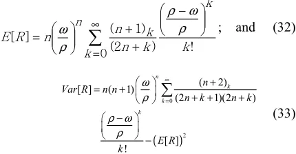
Putting s = 1 and 2 in (31) yields the first two raw moments and thence the mean and variance of R:
! ) 2 (
) 1 ( ]
[
0 n k k
n n
R E
k
k
k
n
−
+ +
=
∑
∞=
ρω ρ
ρ
ω ; and (32)
( )
0
2
( 2) [ ] ( 1)
(2 1)(2 )
[ ] !
n
k k
k
n Var R n n
n k n k
E R k
ω ρ ρ ω
ρ
∞
=
+
= + + + +
−
−
∑
(33)
It is very difficult to evaluate these two moments as the series converge very slowly unless ρ and ω are nearly equal, a rare situation in general. This in turn precludes us from applying direct analytic methods to study the distributional characteristics of the reliability rate.
6. Conclusion
This paper has attempted to model the maximum likelihood estimation of reliability rate and the related statistical properties. Some of the empirical expositions of the reliability analysis presented here have already been done (for example,[2], [5], [6]), while this paper serves as a theoretical background. We present the instantaneous and long run reliability rate (and its complement outage rate) in the framework of a Markov process and consider its Maximum Likelihood estimate. From this we derive the density function of reliability rate and thence its moments. The major conclusion here is that the expression we have derived for analyzing the distributional properties of the reliability rate is less amenable to empirical estimation.
References
[1] Bazovsky, Igor (1961) Reliability Engineering and Practice. Prentice hall Space Technological series, Prentice Hall, Englewood Cliffs, NJ.
[2] Pillai, N. Vijayamohanan, (1991), Seasonal Time-of-Day Pricing of Electricity under Uncertainty - A Marginalist Approach to Kerala Power System. Ph. D. Thesis. University of Madras. Ch.4.
[3] Zehna, P. (1966), `Invariance of Maximum Likelihood Estimation', Annals of Mathematical Statistics, Vol. 37, p. 744. [4] Kendall, M. G., and Stuart, A., (1967), The Advanced Theory
of Statistics, Vol. II, 2nd Edition, Hafner, New York. Ch. 18. [5] Pillai, N. Vijayamohanan (1999) “Reliability Analysis of
Power Generation System - A Case Study” Productivity, July – Sept., 1999, Vol 40, No. 2: 310 – 318.
[6] Pillai, N. Vijayamohanan (2002) “Reliability and Rationing Cost in a Power System”, CDS Working Paper No. 325, March. http://cds.edu/download_files/325.pdf
0 0.1 0.2 0.3 0.4 0.5 0.6 0.7 0.8 0.9 1
0.1 0.2 0.3 0.4 0.5 0.6 0.7 0.8 0.9
Reliability Rate (R)
f(
R