Application of the Method of Least Squares to a Solution of the Matched Field Localization Problem with a Single Hydrophone

(1)

University of New Orleans University of New Orleans

ScholarWorks@UNO

University of New Orleans Theses and

Dissertations Dissertations and Theses

8-7-2008

Application of the Method of Least Squares to a Solution of the

Matched Field Localization Problem with a Single Hydrophone

Sean R. Chapin

University of New Orleans

Follow this and additional works at: https://scholarworks.uno.edu/td

Recommended Citation Recommended Citation

Chapin, Sean R., "Application of the Method of Least Squares to a Solution of the Matched Field Localization Problem with a Single Hydrophone" (2008). University of New Orleans Theses and Dissertations. 854.

https://scholarworks.uno.edu/td/854

This Dissertation is protected by copyright and/or related rights. It has been brought to you by ScholarWorks@UNO with permission from the rights-holder(s). You are free to use this Dissertation in any way that is permitted by the copyright and related rights legislation that applies to your use. For other uses you need to obtain permission from the rights-holder(s) directly, unless additional rights are indicated by a Creative Commons license in the record and/ or on the work itself.

This Dissertation has been accepted for inclusion in University of New Orleans Theses and Dissertations by an

(2)

Application of the Method of Least Squares to a Solution of the Matched Field Localization Problem with a Single Hydrophone

A Dissertation

Submitted to the Graduate Faculty of the University of New Orleans in partial fulfillment of the requirements for the degree of

Doctor of Philosophy in

Engineering and Applied Science

by

Sean R. Chapin

B.S. Western Michigan University, 1998 M.S. University of New Orleans, 2001

(3)

ii

Acknowledgements

A special thanks to the co-chairs of my dissertation committee, Dr. George Ioup and Dr.

Juliette Ioup of the Department of Physics at the University of New Orleans. They always had

their door open to provide help and support through this journey, and they were (and are)

outstanding teachers. I'd also like to thank Dr. George Smith of the Naval Research Laboratory

for taking the time to provide guidance on my research. Thank you to the other members of my

dissertation committee for their feedback: Dr. Jinke Tang, Dr. Edit Bourgeois, and Dr. Ken

Holladay.

Infinite thanks to Aisling for putting up with the long hours and for cheering me up when

the going got tough. Thank you to my supervisor Anne for making the completion of this

dissertation possible. Thank you to my co-workers in the RAWG team for giving me the space I

needed to get my research done. Thank you to the U.S. Navy for providing the time and the

funds to complete this project. Finally, thank you to my friends and family for always providing

(4)

iii

List of Figures

`

Figure 1.1a. The LFM source signal ...13

Figure 1.1b. The Green's function ...13

Figure 1.1c. The measured signal ...13

Figure 1.2a. The source signal spectrum ...15

Figure 1.2b. The Green's function spectrum ...15

Figure 1.2c. The measured signal spectrum...15

Figure 1.3a. Magnitude of D/G(X) for the correct source location ...16

Figure 1.3b. Magnitude of D/G(X) for the incorrect source location ...16

Figure 1.4a. The inverse FFT of D/G(X) for the correct source location ...17

Figure 1.4b. The inverse FFT of D/G(X) for the incorrect source location ...17

Figure 1.5. Cross correlation for correct source location...19

Figure 1.6. Cross correlation for incorrect source location ...20

Figure 3.1 (a-f). The source signals in time and frequency domain ...36

Figure 3.2a. Time domain Green's function ...38

Figure 3.2b. Frequency domain Green's function ...38

Figure 3.3 (a-f). Received signals in time and frequency domain ...39

Figure 3.4. Ambiguity plot of new localizer ...40

Figure 3.5. Close up of ambiguity plot of new localizer ...42

Figure 3.6. Analytical and BELLHOP Green's functions for Pekeris waveguide ...43

Figure 3.7 (a-f). Ambiguity plots for 10 Hz source signal bandwidth ...45

(7)

vi

Figure 3.13 (a-f). 60 dB SNR measured signals in time and frequency domains ...55

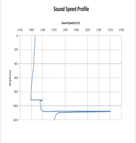
Figure 4.1. Sound speed profile of the water column and the bottom ...63

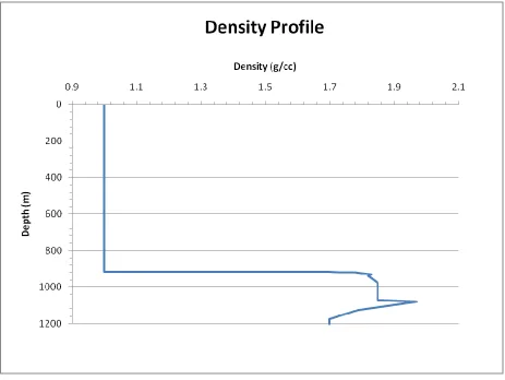
Figure 4.2. Density profile of the water column and the bottom ...64

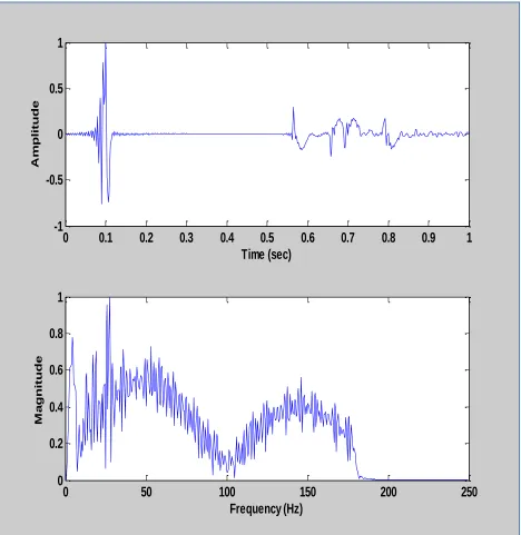
Figure 4.3a. Correlated source signal in the time domain ...66

Figure 4.3b. Correlated source signal in the frequency domain ...66

Figure 4.4a. Correlated measured signal in the time domain for 129 m case ...67

Figure 4.4b. Correlated measured signal in the frequency domain for 129 m case ...67

Figure 4.5a. Green's function in time domain calculated with SPARC for 129 m case ...69

Figure 4.5b. Spectrum of Green's function calculated with SPARC for 129 m case ...69

Figure 4.6. Ambiguity plot of new localizer for 129 m case ...70

Figure 4.7. Ambiguity plots for 129 m case ...72

Figure 4.9a. Correlated measured signal in the time domain for 250 m case ...75

Figure 4.9b. Correlated measured signal in the frequency domain for 250 m case ...75

Figure 4.10a. Time domain Green's function calculated with SPARC for 250 m case ....76

Figure 4.10b. Spectrum of Green's function calculated with SPARC for 250 m case ...76

Figure 4.11. Ambiguity plot of new localizer for 250 m case ...78

(8)

vii

Figure A.2. Ambiguity plots for 10 Hz bandwidth and SNR=60 dB ...84

(9)

viii

List of Tables

Table 1.1. Frazer and Pecholc's localizer values...21

Table 3.1. Localization errors for all SNRs and 10 Hz source signal bandwidth ...59

Table 3.2. Localization errors for all SNRs and 100 Hz source signal bandwidth ...59

(10)

ix

Abstract

The single hydrophone localization problem is considered. Single hydrophone

localization is a special case of matched field localization where measurements from only one

hydrophone are available. The time series of the pressure at the hydrophone is compared with

predicted times series calculated using an ocean acoustic propagation model for many different

source locations. The source location that gives the best match between the predicted time series

and the measurement is assumed to be the correct source location. Single hydrophone

localization algorithms from the literature are reviewed and a new algorithm is introduced. The

new algorithm does not require knowledge of the source signal and does not assume the use of a

particular ocean acoustic model, unlike some algorithms in the literature.

Source location estimates calculated from the new algorithm are compared with ground

truth using simulated ocean acoustic measurements and experimental measurements. Source

location estimates calculated using other algorithms from the literature are shown for

comparison. The simulated measurements use three source signals with bandwidths of 10 Hz,

100 Hz, and 200 Hz and the ocean is modeled as a Pekeris waveguide. The new algorithm

estimates the source location accurately for all three source signals when several of the

localization algorithms from the literature give inaccurate estimates. Gaussian white noise

signals are added to the measured signals to test the impact of signal-to-noise ratio (SNR) on the

algorithm. Four signal-to-noise ratios of 60 dB, 40 dB, 20 dB, and 0 dB are used. The new

algorithm gives accurate source location estimates down to an SNR of 20 dB for two of the

source signal bandwidths. Source location estimates using other algorithms from the literature

(11)

x

Source location estimates are calculated using two hydrophone measurements taken at

different depths in an experiment conducted near the Bahamas. The new algorithm accurately

estimates the source location in both cases. In one case, only two other localization algorithms

from the literature locate the source accurately. In the other case, only one other localization

algorithm succeeds.

(12)

1

Chapter 1. Introduction

1.1 Matched Field Processing

Matched field processing in underwater acoustics refers to methods of using spatial

measurements of the underwater pressure to detect and locate an acoustic source, or to infer

environmental parameters of an ocean waveguide. The large collection of techniques developed

over the last few decades can be traced to Hinich (1973) and Bucker (1976), who developed

algorithms based on comparing spatial measurements of pressure on an array of hydrophones

with the measurements predicted by an ocean acoustic propagation model. The spatial pressure

distribution of the acoustic field is determined by the location of the source and the

environmental parameters such as the sound speed profile of the water and the sound speed in the

ocean bottom. If the environmental parameters are known for a given experiment, they can be

entered into an acoustic propagation model and the pressure distribution can be predicted for

various trial locations of the source. The pressure patterns measured at the hydrophones are then

matched to the patterns estimated by the acoustic model. The basic idea is that the source is

located, or localized, when the predicted acoustic field using the correct source location matches

the measurements of the field at the receivers.

Similar techniques exist for estimating the ocean acoustic environmental parameters such

as the sound speed. In this case the source location is known but the environmental parameters

are unknown. The acoustic propagation model is run for different combinations of

environmental parameters and the resulting pressure patterns are predicted at the hydrophones.

(13)

2

parameters by looking for the best match between the predicted pressures and the measured

pressures. A large body of literature exists on matched field processing and two reviews, with

extensive references, are given by Baggeroer et al. (1993) and Tolstoy (1993).

1.2 Single Hydrophone Localization

In this dissertation we examine a special case of matched field processing where pressure

measurements from only one hydrophone are available to locate a source. The problem is

different from the matched field processing problem described above because we have no

information on the spatial distribution of the acoustic field in our measurements. We assume we

have one time series of the pressure measured at a single point in space where the hydrophone is

located. The location of the source producing the disturbance is unknown, and we assume the

source produces a broadband signal at the hydrophone. The assumption of a broadband source is

necessary because a continuous wave source of a single frequency provides no useful

information on the source location without accompanying spatial measurements. In other words,

a continuous wave source would produce a sine wave of constant amplitude at the receiver,

giving us no insight into the propagation paths of the acoustic energy. If we know the

environmental parameters of the ocean waveguide, we can use ocean acoustic propagation

models to predict the measurement at the hydrophone for different source locations. We call

these replica signals. The location that gives the best match between the replica signal and the

measured time series at the hydrophone is assumed to be the correct location of the source. This

is conceptually similar to matched field processing techniques using arrays of hydrophones.

Single hydrophone localization techniques are important not only for their intrinsic

interest, but also for their computational and experimental simplicity. Using a single hydrophone

(14)

3

the measurements. This gives researchers on tight budgets flexibility to put their resources into

other parts of the experiment if they can do the job with one hydrophone.

In the following sections we define the terminology and notation used throughout the

dissertation. This is followed by a review of the literature on single hydrophone localization

techniques discussing their assumptions and implementations.

1.3 Preliminary Considerations

1.3.1 Equations of Ocean Acoustics

The propagation of sound in the ocean is governed, to a good approximation, by the following

linear inhomogeneous partial differential equation (Jensen, et al. 1994):

, _(1.1)

where p is the pressure, c(z) is the sound speed at depth z, t is time, and s(X,t) is a function

describing the source producing the disturbance at some location X. Ocean acoustic modeling

concerns itself with analytical and numerical techniques of solving equation (1.1) under different

boundary conditions. The solution to the equation will give the time dependent pressure at some

point in the water (e.g., the location of a hydrophone).

The ocean is generally a time varying medium because environmental factors affecting

the ocean are constantly changing. For example, weather conditions, time of day, and the season

all affect the sound speed profile in the ocean. Equation (1.1) shows that the pressure measured

at a point explicitly depends on the sound speed profile. The reason is that the sound will refract

in the ocean as it travels through layers with different sounds speeds. This is analogous to how

light will refract as it travels from one medium to another with a different index of refraction. If

(15)

4

performed, the ocean can be regarded as a time invariant system. The response of any linear

time invariant (LTI) system to a given input can be expressed by a convolution relation

(Bracewell 2000)

(1.2)

where t is the time, s(t) is the source signal (i.e., the input), g(t) is called the Green's function or

impulse response of the system, and p(t) is the pressure measured at the hydrophone (i.e., the

output or response of the system). We have suppressed the spatial dependence of the terms in

the equation for clarity; p(t) is the pressure measured at a location Y, s(t) is the source signal

located at X, and g(t) is a function of both X and Y. Equation (1.2) is the solution of equation

(1.1) expressed as an integral equation. The Green's function g(t) is defined to be the solution of

equation (1.1) when the source function s(X,t) is a delta function. In other words it is the

response of the ocean at Y to a point source located at X emitting a very short duration pulse.

The Green's function depends on the location of the source and the receiver and will generally

change with different source and receiver locations, with one exception. The principle of

reciprocity (Jensen, et al. 1994) states that if the source and receiver locations are interchanged,

the Green's function will not change. This is a key fact that makes localization in ocean

acoustics possible. In solving the localization problem, we can treat the location of our receiver

as the source location in equation (1.1). The source we are trying to locate in our experiment

becomes the receiver in the model. Matched field processing takes advantage of this by

repeatedly solving equation (1.1) for different receiver locations and compares each solution to

our hydrophone measurement. The location that gives the closest match is the location of the

(16)

5

Equation (1.2) provides us the means to model a hydrophone measurement at any

location we choose in an ocean environment. We use ocean acoustic models to solve equation

(1.1) for an impulsive point source and obtain the Green's functions for different source and

receiver locations. The next section will describe two acoustic models we will use in this

dissertation.

1.3.2 Acoustic Propagation Models

There is a wide variety of acoustic propagation models available today to calculate the

Green's functions in an ocean environment. Many of them are based in the frequency domain

where the source function is assumed to be radiating at a single frequency. To form the time

dependent Green's function from these models, the model must be run repeatedly at all

frequencies forming a Green's function in the frequency domain. This function is then inverse

Fourier transformed to the time domain yielding the time dependent Green's function. Other

models solve equation (1.1) directly in the time domain giving the Green's function immediately.

The acoustic models we will use in this dissertation are BELLHOP and SPARC. The

BELLHOP model is a Gaussian beam tracing model (Porter and Bucker 1987) that implements

the ray tracing approximation of acoustics by associating a narrow Gaussian beam with each ray.

The ray approximation models the sound as narrow beams of acoustic energy traveling through

the ocean, similar to the geometric rays used in optics. The advantage of Gaussian beams over

standard ray tracing is that it eliminates unrealistic features such as perfect shadows and caustics

in the acoustic field. BELLHOP is a frequency domain model that assumes a point source

radiating at a single frequency. The radiating point source is approximated by propagating

beams over a range of angles from the source location. Those beams arriving at the receiver

(17)

6

arrival time is a function of the sound speed and the amplitude is a function of both geometrical

spreading and losses of energy from bottom bounces. Two of the single hydrophone localization

techniques in the literature that we will discuss explicitly incorporate the ray approximation into

their algorithms and use BELLHOP for calculations.

In the time domain, the ray approximation gives the received signal as scaled and delayed

replicas of the source signal (Jesus, Porter, et al. 2000; Jensen, et al. 1994). The Green's function

is written as

(1.3)

where m is a ray arrival at the receiver, am is the amplitude of arrival m, and τm is the time at

which arrival m reaches the receiver. The ray model outputs are the arrival times of the rays and

their amplitudes. Once the Green's function is constructed using equation (1.3), it is convolved

with the source function to model the signal at the hydrophone.

The other model we will use is SPARC (SACLANT Pulse Acoustic Research Code), a

time domain acoustic propagation model (Porter 1990, 2008). SPARC is ideally suited for

calculating time dependent Green's functions because the model works in the time domain

solving equation (1.1) directly. A short duration pulse can be input at any location in the model

and allowed to propagate through the ocean. The time dependent Green's function at any desired

location can be extracted to use in localization algorithms. Frequency domain acoustic models

are more cumbersome to deal with because they need to be repeatedly run at the frequencies in

(18)

7

1.3.3 Discrete Time Signal Model

Digital signal processing on experimental data is done with discrete time signals of finite

length. The approximation of equation (1.2) for these signals is (Brigham 1988)

(1.4)

where m and n are integer indices labeling the values of s and g at discrete times m and n.

Equation (1.4) will serve as our fundamental model of the pressure measurement at a

hydrophone throughout this dissertation. A convenient shorthand for equations (1.2) and (1.4) is

(Bracewell 2000)

(1.5)

where the asterisk represents the convolution operation.

Another way to express convolution is in matrix notation (Bracewell 2000)

(1.6)

or for short. The source signal vector s is of length M, the Green's function vector g is of

length N, and G is an M+N-1 by M matrix formed from the elements of g. The convolution

matrix is of full column rank (Tong, Xu and Kailath 1993).

(19)

8

1.3.4 Other Definitions and Notation

The cross correlation of signal s with signal g is defined as

(1.7)

or in pentagram notation (Bracewell 2000)

(1.8)

The cross correlation is useful for comparing two signals. If the two signals are very similar at

lag m as signal g is displaced over signal s, a peak will appear in the cross correlation. This is a

useful tool in matched field processing when comparing a replica signal with a measured signal.

We will use the following definition for calculating the Discrete Fourier Transform Fr of

a discrete time function fk:

(1.9)

Many software packages are equipped with Fast Fourier Transform (FFT) algorithms to calculate

equation (1.9) very efficiently.

An analytic signal is the complex valued signal associated with the real valued

signal f(t) defined by the following Fourier transform pair (Bracewell 2000)

(1.10)

where f is the frequency, H(f) is the unit step function, and F(f) is the Fourier transform of f(t).

The negative frequency portion of the frequency spectrum of f(t) is suppressed by the step

(20)

9

analytic signal is called the envelope of f(t). Intuitively the envelope is the function that

touches the peaks of f(t) showing how the general shape of its amplitude varies with time.

The following two facts about matrix algebra will be used in this dissertation:

1). Given an matrix A, the shortest least squares solution to the linear system Ax = b is

(1.11)

where A+ is the pseudoinverse of the matrix A (Strang 1993).

2). If the rank of the matrix A is n (A is full column rank), then A+A=In where In is the

identity matrix (Lutkepohl 1996).

The p-norm of a vector f is defined as

(1.12)

One exception to this notation is for the square of the 2-norm, i.e., the sum of the squares of the

elements of a vector. We will omit the subscript in those cases because it is easier to read and it

is consistent with notation used in the literature,

(1.13)

The -norm of the vector f is

(21)

10

1.4 Literature Review of Single Hydrophone Localization

1.4.1 Li and Clay (1987)

In 1987 Li and Clay (Clay 1987, Li and Clay 1987) proposed a localizer using the cross

correlation function. They construct replica signals by convolving the Green's functions for

different source locations with the source signal. Then they cross-correlate the replica signals

with the measured signal over a grid of trial source locations. The cross-correlation peaks at the

true source location because the replica signal closely matches the measured signal. The

equation describing this in our notation is

(1.15)

where t is the time, X is a trial source location, h(X,t) is the replica signal for location X, and d(t)

is the measured signal. The function in the brackets is calculated for all trial source locations and

the location X corresponding to the maximum value of the bracketed function is the estimate of

the source location.

1.4.2 Frazer and Pecholcs (1990)

The Frazer and Pecholcs technique (Frazer and Pecholcs 1990) is distinct from the others

because it does not rely on a measurement or estimate of the source signal. The information

required is the measured signal at the hydrophone and the predicted Green's functions for each

trial source location. Frazer and Pecholcs (1990) proposed a family of localizers listed below.

The notation is as follows: h(X) is the replica signal for trial source location X, d is the measured

signal, D is the FFT of the measured signal, is the Green's function for source location X,

and G(X) is the FFT of the Green's function for source location X. A discussion of the localizers

(22)

11

(1.16)

(1.17)

(1.18)

(1.19)

(1.20)

(23)

12 where is the inverse FFT of D/G(X).

(1.22)

where .

The first thing we want to point out is that the localizer is the same as the one

developed by Li and Clay described in the previous section. The and localizers are

variations of this with different normalization factors in the denominator. The norm works in

the time domain on the inverse FFT of the Fourier deconvolution. The

localizers all work in the frequency domain on the Fourier deconvolution of D and G(X). The

idea is that the Fourier deconvolution D/G(X) will give an estimate of the source signal spectrum,

assumed to be smooth compared to G(X). G(X) typically has many nulls in it for underwater

acoustic problems. If the correct G(X) is put in, the resulting Fourier division will be relatively

smooth. When the incorrect G(X) is put in, the division will result in a spiky spectrum because

of the nulls of G(X) in the denominator. This drives the value of the norm of the division higher

when G(X) is not correct. If the norm of the division is put in the denominator of the localizer

function, then the localizer will reach a peak value at the true source location.

To gain a better understanding of how the Frazer and Pecholcs localizers work, we will

go through a numerical example comparing the values of the localizers when the trial source

location is correct with when it is incorrect. Figure 1.1 shows the source signal, Green's

function, and measured signal we will use for this example. The source signal is a linear

(24)

13

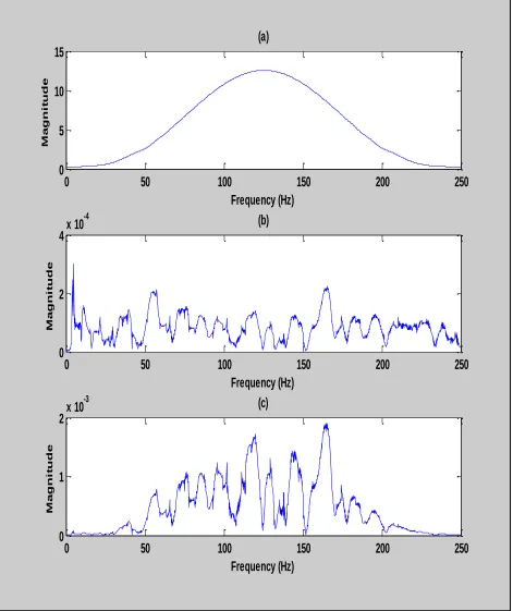
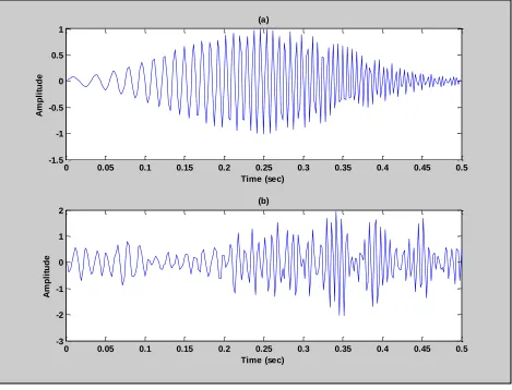
Figure 1.1 (a)The source signal. (b) Green's function. (c) Measured signal.

0 0.05 0.1 0.15 0.2 0.25 0.3 0.35 0.4 0.45 0.5

-1 0 1

Time (sec)

A

m

pl

i

t

ud

e

(a)

0 0.05 0.1 0.15 0.2 0.25 0.3 0.35 0.4 0.45 0.5

-5 0 5x 10

-5

Time (sec)

A

m

pl

i

t

ud

e

(b)

0 0.1 0.2 0.3 0.4 0.5 0.6 0.7 0.8 0.9 1

-1 0 1

Time(sec)

A

m

pl

i

t

ud

e

(25)

14

modulated with a Hamming window and the duration of the signal is 0.5 seconds. The sampling

interval is 0.002 seconds, giving a cutoff frequency of 250 Hz. The Green's function is

representative of what would be found in a shallow underwater acoustic environment. Notice

that there are several arrivals representing reflections of the source signal energy from the ocean

surface and the bottom. The measured signal was calculated by convolving the source signal

with the Green's function. In this case the Green's function significantly distorts the source

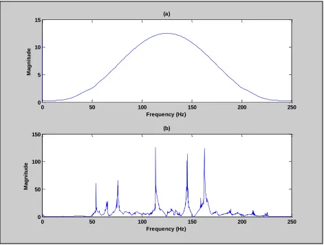
signal on its way to the receiver. Figure 1.2 shows the energy spectra of the source signal,

Green's function, and measured signal in the frequency domain. The source signal spectrum is

very smooth and centered at 125 Hz. The Green's function spectrum is irregular in shape and

features a number of nulls. By the convolution theorem (Bracewell 2000), the spectrum of the

measured signal is the product of the source spectrum and the Green's function spectrum. The

irregular shape and the nulls of the Green's function show in the frequency band where the

source signal is most prominent.

The next task is to calculate the Frazer and Pecholcs localizer functions when the correct

Green's function from Figure 1.1 is used, and for an incorrect Green's function corresponding to

a different source location. Figure 1.3 shows the result of D/G(X) for each case where D is the

measured signal spectrum and G(X) is the Green's function. When the correct Green's function is

used, the smooth spectrum of the source signal is deconvolved out. If the incorrect Green's

function is used, a spectrum with a number of large peaks results. These peaks are there because

the nulls in the spectrum of the Green's function cause large values in the division operation

where there are not corresponding nulls in the measured signal's spectrum. This is the essential

feature for understanding Frazer and Pecholc's frequency domain based localizers. The Fourier

(26)

15

Figure 1.2. (a) The source signal spectrum. (b) Spectrum of Green's function, (c) Spectrum of measured signal.

0 50 100 150 200 250

0 5 10 15

Frequency (Hz)

M

a

gn

i

t

ud

e

(a)

0 50 100 150 200 250

0 2 4x 10

-4

Frequency (Hz)

M

a

gn

i

t

ud

e

(b)

0 50 100 150 200 250

0 1 2x 10

-3

Frequency (Hz)

M

a

gn

i

t

ud

e

(27)

16

Figure 1.3. (a) Magnitude of D/G(X) for the correct source location; (b) magnitude of D/G(X) for the incorrect source location

locations as those in the measured signal's spectrum can prevent these large peaks from

appearing.

To understand the time domain localizer we need to look at the inverse FFT of these

Fourier deconvolutions to see what happens in the time domain. Figure 1.4 (a) shows the result

when the correct Green's function is used. The Hamming windowed LFM pulse is retrieved just

as the frequency domain picture in Figure 1.3 (a) suggested. Figure 1.4 (b) shows the recovered

signal with the incorrect Green's function. An irregular function results bearing little

resemblance to the original source signal. The localizer works on a different principle than

0 50 100 150 200 250

0 5 10 15

Frequency (Hz)

M

a

gn

it

ud

e

(a)

0 50 100 150 200 250

0 50 100 150

Frequency (Hz)

M

a

gn

it

ud

e

(28)

17

Figure 1.4. (a) The inverse FFT of D/G(X) for the correct source location; (b) the inverse FFT of D/G(X) for the incorrect source location shown in Figure 1.3(b).

the frequency domain localizers. It is sensitive to the duration of the signal in the time domain.

Shorter duration source signals tend to give lower values in the denominator of this localizer. If

the original source signal is sufficiently compressed in the time domain, this localizer will have

higher values when the deconvolution is correct. As Figure 1.4 (b) shows, the incorrect result

gives a ragged and spread out signal estimate that tends to decrease the value of the localizer.

We are now left to discuss the χ and μ localizers. These localizers work with the cross

correlation of the replica signal with the measured signal. They are the only localizers in the

0 0.05 0.1 0.15 0.2 0.25 0.3 0.35 0.4 0.45 0.5 -1.5

-1 -0.5 0 0.5 1

Time (sec)

A

m

pl

it

ud

e

(a)

0 0.05 0.1 0.15 0.2 0.25 0.3 0.35 0.4 0.45 0.5 -3

-2 -1 0 1 2

Time (sec)

A

m

pl

it

ud

e

(29)

18

family that rely on knowledge of the source signal for their calculation. The localizer is

idential to the Clay localizer; and are similar but with different normalizations. Figure

1.5 shows the cross correlation with the incorrect Green's function; Figure 1.6 shows the cross

correlation with the correct Green's function. Qualitatively both waveforms look similar

suggesting these localizers are less sensitive to the different Green's functions. The peak value

of the cross correlation and the 1-norms are similar too. The similarity of the localizers suggests

that a calculation of the localizers over all source locations could result in many false peaks.

The results in Table 1.1 summarize the values of the Frazer and Pecholc's localizer

functions for our sample case. All of the localizers in this example showed higher values at the

correct location except the localizer. Both the χ and μ localizers are based on the cross

correlation of the replica signal with the measured signal but have different normalization

factors. The failure of the μ localizer but not the χ localizers suggests that the normalizations

used in these localizers are very important. Notice the strong differences between the θ and φ

localizers. Those are sensitive to the smoothness of the source signal spectrum estimate from the

Fourier division. The assumption that the source signal spectrum be smooth compared to G(X) is

important for these localizers.

1.4.3 Lee (1998)

The next localizer we will look at is by Lee (1998) and is another one based on cross

correlation. The source signal is assumed to be known and the Green's function is measured

directly by calculating the cross correlation of the measured signal and the source signal, as in

equation (1.7). The result of this calculation is equivalent to the received signal resulting from

the transmission of the autocorrelation of the source signal through the ocean environment.

(30)

19

Figure 1.5. The cross correlation of the replica signal with the measured signal for the incorrect source location.

0 0.2 0.4 0.6 0.8 1 1.2

-1.5 -1 -0.5 0 0.5 1 1.5x 10

-7

Time (sec)

A

m

pl

it

ud

(31)

20

Figure 1.6. The cross correlation of the replica signal with the measured signal for the correct source location.

0 0.2 0.4 0.6 0.8 1 1.2

-1.5 -1 -0.5 0 0.5 1 1.5x 10

-7

Time (sec)

A

m

pl

it

ud

(32)

21

Localizer Incorrect Source Location Correct Source Location

0.2267 0.2784

0.0011 0.0014

0.0091 0.0079

0.0404 0.4409

113.4 889.0

0.0051 0.0118

0.0003 0.0004

Table 1.1. Frazer & Pecholcs localizer values for the correct and incorrect source locations.

should give a good approximation of the Green's function. The Green's function estimate can

then be directly compared to the Green's functions calculated from an acoustic propagation

model using the cross correlation again. The localizer will reach a peak value when the

estimated Green's function most resembles the Green's function from the model corresponding to

the correct source location. This localizer is very similar to the Clay localizer except that the

cross correlation is calculated between the Green's functions, rather than between a replica signal

and the measured signal. Here is the Lee localizer in our mathematical notation:

(33)

22

where is the Green's function estimate from cross correlating the measurement with the source

signal, and ) is the Green's function calculated from the acoustic propagation model for

location X.

1.4.4 Porter et al. (1998)

Porter et al. (1998) developed another localizer based on the cross correlation of the

measured signal with a replica signal with one important difference from the previous localizers

we've looked at: they cross correlate the logarithm (log10) of the envelopes of the replica signal

and measured signal rather than the signals themselves. The principle behind this is that in many

environments only the first few arrivals at the receiver dominate the measured signal energy.

The later arrivals are attenuated more from multiple bottom interactions on their journey to the

receiver. The localizers by Porter et al. use the envelope of the signals to put less emphasis on

the fine details of the signal. They use the logarithm to emphasize the larger energy portions of

the signal. The hypothesis is that the localizer will be more robust. The equation is as follows

(1.24)

where rle is the logarithm of the envelope of the measured signal and is the logarithm of

the envelope of the replica signal for location X. Again we calculate the replica signal over all

trial source locations X and look for where the localizer peaks.

1.4.5 Jesus et al. (2000)

The localizers developed by Jesus et al. (Jesus, Porter, et al. 1998, 2000) are the first

we've discussed that explicitly assume that the acoustic propagation model used is a ray tracing

model (they used BELLHOP). This is often desirable because ray models run very quickly and

(34)

23 First we define some notation:

X: the source location.

y: measurement signal vector at the hydrophone.

S[τ(X)]: matrix of source signal replicas; each column contains one replica of the source signal

delayed by an amount defined by τ(X).

τ(X): vector defining arrival times from a ray based acoustic propagation model for source

location X.

a(X): amplitude vector defining amplitudes of arrivals from ray based acoustic propagation

model for source location X.

ε: random noise vector (representing measurement noise).

The signal model is

(1.25)

The received signal model is composed of scaled and delayed replicas of the source signal as

predicted by acoustic ray theory. The localizer calculates the product of the measurement signal

vector y with the matrix S. The resulting vector's elements are squared and summed for all trial

source locations. In other words, they calculate the inner product of the measurement vector

with scaled and delayed replicas of the source signal. The idea is that the localizer will peak

when the τ(X) time delay vector has the correct arrival times in it corresponding to the true

source location. The localizer equation is written

(1.26)

where X is the source location and H is the Hermitian transpose (complex valued signals are

admissible). Jesus et al. generalize their localizers to the case of N snapshots of the measured

(35)

24

to use in the algorithm. We will not be looking at this case, however, and will focus on the case

where only a single measurement is available.

1.4.6 Tiemann et al. (2006)

A recent paper by Tiemann et al. (2006) looked at marine mammal localization with a

single hydrophone. Ray theory was explicitly assumed for this technique by assuming source

signal arrivals in the measurement can be clearly identified. Localization is done by matching

arrival times estimated from the measured signal to arrival times calculated from a ray tracing

model. The sperm whale clicks they measured were broadband and of very short duration. The

ray model of propagation is ideal for signals like this and arrivals at the receiver can be easily

identified. Their method was to match the arrivals at the receiver to the arrivals calculated by a

ray propagation model (they used BELLHOP). To do the matching, they created bins with a

width of 15 milliseconds across the length of the measurement and the arrival time vector from

the ray model. They considered any arrivals in a particular bin that are present in both the

measured signal and the calculated arrivals to be overlapping. This process is continued across

the entire measurement tabulating the overlaps. If there are arrivals that do not overlap in a bin,

they are considered nonoverlapping and those are tabulated. A net overlap score is calculated by

summing the overlaps and then subtracting the sum of the nonoverlapping arrivals. The score is

calculated for each trial source location. The location with the highest net overlap score is the

location of the source.

This technique is similar to other techniques where ray arrival times in the measurement

are compared to those calculated by a model. Instead of calculating a cross correlation as in

many of the methods described above, or through matrix algebra, Tiemann et al. (2006) use a

(36)

25

1.4.7 Other Localization Techniques

There are other papers in the literature that use geometric ray tracing techniques to

calculate the ray arrival times at a hydrophone for different source locations (Hassab 1976; Cato

1998; Aubauer, Lammers and Whitlow 2000). This would be a useful technique for broadband

source signals in environments that can be approximated by a constant sound speed profile. A

paper by Unpingco et al. (1999) describes a synthetic aperture technique for tracking moving

sources under certain assumptions. Kuperman and D'Spain (2001) describe a technique for

localizing in range only for broadband sources in deep water. We will not examine these

(37)

26

Chapter 2 A New Technique for Single Hydrophone Localization

2

.1 Description

Although we described several approaches to single hydrophone localization from the

literature, the amount of work done on single sensor localization is small when compared to the

voluminous literature on matched field processing with multiple receivers. Most of the methods

we described from the literature are variations on the basic idea of comparing replica signals

generated using the source signal and an acoustic model, with the measurement at the receiver.

A maximum or a minimum in the resulting metric is used to quantify the correlation and

determine the true source location. All of the above methods, except the algorithm by Frazer and

Pecholcs (1990), rely on knowledge of the source signal that is transmitted, and this might be a

limitation in some situations where this information may not be available or easily obtained.

We propose a new single hydrophone localization algorithm using the method of least

squares. Least squares is well established and can be implemented efficiently using matrix

algebra packages. This algorithm does not require knowledge of the source signal. The Green's

function estimate can be calculated from any acoustic propagation model. There is no

assumption built into the new algorithm requiring that a particular model be used (e.g., a ray

model). This frees up researchers to use any model that is appropriate for their experiment and it

gives them options to balance their resources. This can be important because some propagation

(38)

27

2.2 Algorithm

First we will establish some notation and then lay out the steps of the algorithm. Recall

equation (1.6) describing a discrete time LTI system for underwater acoustics

(2.1)

where G is the convolution matrix of the Green's function for a source and receiver in the

environment of the experiment, s is the discrete time source signal vector, and m is the

measurement vector at the receiver. Generally there will be some interfering noise that we will

model as a random vector n added to the measurement vector

(2.2)

We know the location of our receiver but do not know the location of the source. Using the

environmental information our propagation model requires, such as the sound speed profile of

the water, we can calculate a set of trial Green's functions over a grid of possible source

locations. Each trial Green's function represents the propagation characteristics for a particular

source and receiver geometry. For example, in a two dimensional problem where the

coordinates are range and depth, we can calculate the Green's functions over a rectangular grid of

ranges and depths where the source might be located. If the grid is sufficiently large to include

the source, our algorithm should identify the range and depth of its location. The source signal is

assumed to be unknown. The question is how can we find the location without knowing either

the signal or the Green's function? The answer is that we will simultaneously estimate the source

(39)

28

(2.3)

is a trial Green's function from our search grid and is our estimate of the source signal that

we obtain by solving the equation:

(2.4)

is the pseudo-inverse of . The pseudo-inverse creates the shortest least squares solution to

the problem, as we pointed out in equation (1.11). Now that we have our source signal estimate

, we can use it to calculate a replica signal , assuming that is the correct Green's function:

(2.5)

To summarize the last few steps, we create a replica signal by temporarily assuming that our trial

Green's function is the correct one. Then we estimate the source signal using the least squares

solution to equation (2.3). The resulting least squares estimate of the source signal is then

convolved with the trial Green's function in equation (2.5) to give us a replica signal . The

final step is to compare our replica signal with the measured signal and calculate the squared

difference between them:

(2.6)

The process in equations (2.4) through (2.6) is repeated for every trial source location X. The

localizer function is denoted

(2.7)

The localizer will achieve a minimum value when the Green's function corresponding to the

(40)

29

2.3 Analysis of Algorithm

There are two possibilities when a trial Green's function is input into the algorithm:

either it is the correct Green's function describing the system or it is not.

Case 1: (the Green's function for the correct source location is used). Substituting

into equation (2.4) gives

(2.8)

Recall from equation (2.2) that and substitute it into equation (2.8):

(2.9)

Assuming that the signal to noise ratio is high enough to render the contribution of the second

term to be negligible, we have

(2.10)

Using the fact that if and only if G is full column rank (Lutkepohl 1996), eq. (2.10)

becomes

(2.11)

Finally we have for the replica signal vector

(2.12)

(41)

30

(2.13)

Case 2: (a Green's function for an incorrect source location is used). Substituting

equation (2.2) into equation (2.4) gives

(2.14)

where we assume again that the noise term n is negligible and neglect that term.

The replica signal vector becomes,

(2.15)

The matrix product for a full column rank matrix (Lutkepohl 1996). The product is

equal to the identity matrix only when the system is full row rank (Lutkepohl 1996). Calculating

the difference between the measured signal and the replica signal gives

(2.16)

We simplify equation (2.16) into a more convenient form:

(2.17)

Therefore in Case 2 showing that our localizer should achieve a minimum only when

the Green's function for the correct source location is put into the algorithm. The assumptions

we made in equations (2.10) and (2.14) that the noise vector n is small is important and we will

look at the impact of a larger n in Chapter 3.

Another notable case is when the Green's function has very few arrivals close together in

(42)

31

When this happens the Green's function resembles a delta function and therefore the convolution

matrix will resemble an identity matrix. In other words, there is not much distortion of the

source signal on its way to the receiver. Inspection of equation (2.3) shows that the source signal

estimate will be very close to the measured signal. This will propagate through the algorithm

and give a replica signal that is very close to the measured signal. The localizer output will take

on very small values in these cases and give unreliable location estimates. Cases like this could

pose a problem for any single hydrophone localization algorithm because they all generally rely

on multiple interactions of the source signal energy with the surface and the bottom. To function

properly, these algorithms require unique Green's functions for different source and receiver

geometries. Researchers must be aware of this in their experimental planning and should try to

put the hydrophone in an advantageous position. It is also important to keep this case in mind

when interpreting the localization data.

2.4 Discussion

The algorithm we've described is based on solving the least squares problem, giving it the

benefit of the fast algorithms that have been developed over the years. The Levinson-Durbin

recursion (Levinson 1947; Durbin 1960) is a very popular algorithm used to solve equation (2.3)

in a computationally efficient and stable manner. Another benefit is that the least squares

formulation naturally accommodates the presence of some random noise in the measured signal.

Least squares finds a solution to minimize and therefore will minimize the effects of the

noise vector n (Strang 1993).

Our algorithm makes no assumptions about the nature of the source signal. Only four of

(43)

32

require no knowledge of the source signal. However Frazer and Pecholcs do make assumptions

on the smoothness of the source signal spectrum and on its duration in the time domain for one

of their localizers. This potentially limits the application of their localizer if the source signal

does not meet their assumptions. Although Tiemann et al. (2006) and other localizers based on

ray arrival times do not explicitly rely on knowledge of the source signal, they do make the

assumption that the source signal is of a wide enough bandwidth that distinct arrivals are

measured at the hydrophone. We propose our localizer as the only one among the ones we've

reviewed in this dissertation that is both model independent and source signal independent.

As with any matched field processing algorithm, our algorithm shares the same potential

sensitivity to inaccuracies in the acoustic modeling. This could be caused by the inaccuracies in

the model itself or by coarse environmental information fed into the model. Researchers should

also experiment with the search grid of trial source locations to determine the appropriate grid

spacing. There may be a balance of the fineness of the grid required for localization and the

computational resources available to run the algorithm over the whole grid.

2.5 Analysis Plan

In the next chapter we present results from simulation data to explore the capability and

sensitivity of our new algorithm. First we look at an initial case with simulated data to

demonstrate the algorithm in a simple environment and compare it with the other localizers

described in Chapter 1. Sensitivities we explore parametrically include signal to noise ratio and

source signal bandwidth. With that understanding, we test the localization algorithm on some

experimental ocean acoustic data to show it can be successfully used in a real ocean

(44)

33

Chapter 3 Simulation Results

3.1 Introduction

In this chapter we test the new method developed in Chapter 2 on some simulated data

sets, look at some of its sensitivities, and compare its localization accuracy to the existing

techniques described in Chapter 1. To minimize any possible biases from the particular acoustic

propagation model selected, we use a closed form analytical solution to the Pekeris waveguide

problem (Pekeris 1948; Jensen, et al. 1994) to calculate the Green's functions. We look at the

sensitivity of our localization algorithm to source signal bandwidth and signal to noise ratio

(SNR).

The source signal is a linear frequency modulated pulse described by the following

equation:

(3.1)

where t is the time, w(t) is the amplitude, f1 is the frequency at which the sweep begins and k is a

constant that determines the rate of increase of the sweep. The instantaneous frequency fi at time

t is given by fi (t) = f1 + kt. The frequency of the signal increases linearly as a function of time.

The constants f1 and k can be chosen to get the desired frequency sweep over the period of the

signal. We choose a Hamming window (Harris 1978) for the amplitude function w(t),

(3.2)

The Hamming window smoothes the sharp rise and fall of the amplitude of the LFM pulse

(45)

34

window to use because it is a built in function of Matlab, the software package we used to do

most of the calculations in this dissertation.

The ocean environment we simulate is a Pekeris waveguide (Pekeris 1948; Jensen, et al.

1994), a model of a single water layer over an infinitely deep fluid bottom layer. Each layer is

characterized by a sound speed and a density. Although the Pekeris waveguide model may be

too simple an approximation for some environments, we use it here to simplify the computations

and to minimize biases that may creep into the sensitivity analysis from assumptions built into

the particular acoustic propagation model used to calculate Green's functions. The Pekeris

waveguide model is well understood and has a relatively simple closed form solution. This

makes the Green's function calculations simple and fast over a grid of trial source locations.

The Green's function is synthesized from the following frequency dependent solution to

the Pekeris waveguide problem (Pekeris 1948; Jensen, et al. 1994):

(3.3)

where r is the range of the receiver, z is the depth of the receiver, zs is the source depth, D is the

water depth, f is the source frequency, krn is the radial wave number of mode n, and kzn is the

vertical wave number of mode n. To obtain the time dependent Green's function, we calculate

Equation (3.2) at every discrete frequency f over the bandwidth defined by the problem and take

the inverse FFT of the result. This process is repeated for every trial source location and the

Green's functions are stored for input into the localization algorithm. For our experiment, we

used the following parameters to characterize the waveguide:

(46)

35 Receiver depth z: 150 meters.

Receiver range: 2100 meters.

Water depth D: 300 meters.

Sound speed in the water: 1500 meters/second.

Sound speed in the bottom: 1650 meters/second.

Density of the water: 1 kg/m3.

Density of the bottom: 1.9 kg/m3.

The sound speed and density of the bottom are representative of a sandy bottom and the water

depth is shallow enough to allow for many interactions of the sound in the water column with the

bottom. The grid over which we calculated the trial Green's functions began at a range of 500

meters from the receiver and went out to 3000 meters, at intervals of 10 meters. The grid

extended over the entire 300 meter water column at intervals in depth of 2 meters.

To simulate the signal measurement at the hydrophone, we convolved the Green's

function for the true source location using equation (3.2) with the source signal from equation

(3.1). We input the result into the localization algorithms as the measured signal. Figure 3.1

shows the three source signals we used, each with different bandwidths. Different bandwidths

were achieved by adjusting the constants f1 and k in equation (3.1). The first bandwidth was a 10

Hz LFM sweep from 120 Hz to 130 Hz. The second bandwidth was a 100 Hz sweep from 75 Hz

to 175 Hz. The third bandwidth was a 200 Hz sweep from 25 Hz to 225 Hz. The durations of

(47)

36

Figure 3.1. The source signals in the time domain and frequency domain. (a) Time domain view of 10 Hz LFM sweep over 0.5 seconds; (b) Frequency domain view of 10 Hz LFM sweep from 120 Hz to 130 Hz; (c) Time domain view of 100 Hz LFM sweep over 0.5 seconds; (d) Frequency domain view of 100 Hz LFM sweep from 75 Hz to 175 Hz; (e) Time domain view of 200 Hz LFM sweep over 0.5 seconds; (f) Frequency domain view of 200 Hz LFM sweep from 25 Hz to 225 Hz. All of the signals are modulated by a Hamming window.

0.1 0.2 0.3 0.4 0.5

-0.5 0 0.5 (a) A m p li t u d e

0 50 100 150 200 250

0.2 0.4 0.6 0.8 1 (b) M a g n it u d e

0.1 0.2 0.3 0.4 0.5

-0.5 0 0.5 (c) A m p li t u d e

0 50 100 150 200 250

0.2 0.4 0.6 0.8 1 (d) M a g n it u d e

0.1 0.2 0.3 0.4 0.5

-0.5 0 0.5 Time (sec) (e) A m p li t u d e

0 50 100 150 200 250

(48)

37

different bandwidths is to test the sensitivity of our new algorithm to the bandwidth of the source

signal, and to compare this sensitivity with that of the other localizers we described in Chapter 1.

Bandwidth is an essential consideration in the single hydrophone localization problem because

we are trying to exploit variability of the Green's function with frequency to locate the source.

The more frequencies we have available in our data, the greater the chance we can calculate

unambiguous replica signals and locate the source.

Figure 3.1 shows the time domain and the frequency domain representations of the three

LFM source signals we use. Figure 3.2 shows the Green's function for the correct source and

receiver pair calculated from equation (3.3) in the time domain and the frequency domain.

Notice the presence of multiple spikes in the time domain representing reflections of the sound

from the surface of the water and the bottom. The frequency domain plot illustrates that the

interaction of the sound with the surface and the bottom strongly attenuates some frequencies,

but not others. Figure 3.3 shows the convolution of each of the source signals with the Green's

function in both the time and the frequency domain. There is significant distortion of the source

signal when it travels to the receiver because of the multiple interactions with the surface and the

bottom. It is the uniqueness of this distortion for each source and receiver pair that we want to

exploit in the localization problem.

3.2 Source Signal Bandwidth Parameterization

3.2.1 10 Hz Source Signal Bandwidth

The first case we look at is the localization results for the 10 Hz LFM sweep from 120

Hz to 130 Hz. Figure 3.4 shows the ambiguity plot for this case using our localization algorithm.

(49)

38

Figure 3.2. (a) Time domain view of the correct Green's function; (b) Frequency domain view of the correct Green's function.

0 0.05 0.1 0.15 0.2 0.25 0.3 0.35 0.4

-1 -0.5 0 0.5 1

Time (sec)

A

m

p

li

tu

d

e

0 50 100 150 200 250

0 0.2 0.4 0.6 0.8 1

Frequency (Hz)

M

a

g

n

itu

d

(50)

39

Figure 3.3. The receiver signals calculated by convolving the source signals in Figure 3.1 with the Green's function in Figure 3.2. (a) Time domain measured signal for the 10 Hz LFM sweep; (b) Frequency domain measured signal for 10 Hz LFM sweep; (c) Time domain measured signal for the 100 Hz LFM sweep; (d) Frequency domain measured signal for the 100 Hz LFM sweep; (e) Time domain measured signal for the 200 Hz LFM sweep; (f) Frequency domain measured signal for the 200 Hz LFM sweep.

0.2 0.4 0.6 0.8

-1 -0.5 0 0.5 (a) A m p li t u d e

0.2 0.4 0.6 0.8

-0.5 0 0.5 1 (c) A m p li t u d e

0.2 0.4 0.6 0.8

-0.5 0 0.5 1 Time (sec) (e) A m p li t u d e

0 50 100 150 200 250

0.2 0.4 0.6 0.8 1 (b) M a g n it u d e

0 50 100 150 200 250

0.2 0.4 0.6 0.8 1 (d) M a g n it u d e

0 50 100 150 200 250

(51)

40

Figure 3.4. Ambiguity plot of our new single hydrophone localization algorithm over a grid of trial source locations for the 10 Hz case. The colors correspond to the reciprocal of the value of the localizer function in each bin. The peak of the localizer function occurs at a range of 2100 meters and a depth of 100 meters. The true location of the source is a range of 2100 meters and a depth of 99 meters.

Peak Value -- Range: 2100 m Depth: 100 m

Range (m)

D

e

p

th

(m

)

500 1000 1500 2000 2500 3000

50

100

150

200

250

(52)

41

of the source and range of the source from the receiver. We plotted the reciprocal so that the

peak value will represent the source location estimate, to be consistent with the other localizers

we discussed in Chapter 1. Our grid spacing was 10 meters in range and 2 meters in depth.

There is a clear peak at a range of 2100 meters and a depth of 100 meters. Recall that the true

location of the source is at a range of 2100 meters and depth of 99 meters. The localizer

successfully located the source within 1 meter despite the source being slightly off of the grid of

trial source locations, and having only a 10 Hz signal bandwidth. Note that localization within 1

meter is the best possible because of the discrete grid of locations over which the calculations are

done. Figure 3.5 gives a close up view of the localizer peak and shows that the peak quickly

tapers off in both range and depth. The peak drops off within about 20 meters in range and 4

meters in depth.

We now consider the performance of the other single hydrophone localizers for

comparison. One issue to consider first is that the localizers by Jesus et al. (2000) and Tiemann

et al. (2006) require their Green's functions be calculated using a ray model. We used

BELLHOP to do this by modeling the Pekeris waveguide using a constant sound speed profile in

the water column and a constant sound speed in the bottom. Figure 3.6 overlays the analytical

Green's function for the Pekeris waveguide with the estimated ray arrivals from BELLHOP.

There is good agreement between the two models in timing and sign for many of the arrivals.

There are two arrivals in the 0.2 to 0.25 second range where BELLHOP's estimate is misaligned

in time and opposite in sign to the analytical solution. These disagreements are not surprising

because the ray approximation of acoustics is most accurate with broadband, high frequency

Application of the Method of Least Squares to a Solution of the Matched Field Localization Problem with a Single Hydrophone

ScholarWorks@UNO

ScholarWorks@UNO

Application of the Method of Least Squares to a Solution of the

Application of the Method of Least Squares to a Solution of the

Matched Field Localization Problem with a Single Hydrophone

Matched Field Localization Problem with a Single Hydrophone

Acknowledgements

Table of Contents

List of Figures

List of Tables

Abstract

Chapter 1. Introduction

1.1 Matched Field Processing

1.2 Single Hydrophone Localization

1.3 Preliminary Considerations

1.4 Literature Review of Single Hydrophone Localization

Chapter 2 A New Technique for Single Hydrophone Localization

2

.1 Description

2.2 Algorithm

2.3 Analysis of Algorithm

2.4 Discussion

2.5 Analysis Plan

Chapter 3 Simulation Results

3.1 Introduction

3.2 Source Signal Bandwidth Parameterization