Discrete Galerkin Method for Higher Even-Order Integro-Differential
Equations with Variable Coefficients
M. Gholipour
Department of Mathematics, Faculty of Basic Sciences,
Sahand University of Technology, Tabriz, Iran. E-mail:m [email protected].
P. Mokhtary∗
Department of Mathematics, Faculty of Basic Sciences,
Sahand University of Technology, Tabriz, Iran. E-mail:[email protected], [email protected]
Abstract This paper presents discrete Galerkin method for obtaining the numerical solution of higher even-order integro-differential equations with variable coefficients. We use the generalized Jacobi polynomials with indexes corresponding to the number of ho-mogeneous initial conditions as natural basis functions for the approximate solution. Numerical results are presented to demonstrate the effectiveness and wellposedness of the proposed method. In addition, the results obtained are compared with those obtained by well known Pseudospectral method, thereby confirming the superiority of our proposed scheme.
Keywords. Discrete Galerkin method, Generalized Jacobi polynomials, Higher even-order Integro-Differential
Equations.
2010 Mathematics Subject Classification. 34A08; 65L60.
1. Introduction
In this paper we develop a discrete Galerkin method for obtaining the numerical solution of the following higher even-order integro-differential equations with variable coefficients
y(2m)(x) +2mP−1 k=0
a2m−k(x)y(k)(x) =f(x) + R
I
K(x, t)y(t)dt,
y(i)(−1) =y(i)(1) = 0 0≤i≤m−1, m∈N, x, t∈I= [−1,1],
(1.1)
where {ai(x)}i2=1m and f(x) are given continuous functions and K(x, t) is a given
smooth kernel function. HereN is the collection of all natural numbers and y(x) is the unknown solution.
Received: 18 June 2015 ; Accepted: 1 September 2015. ∗Corresponding author.
Many mathematical formulation of physical phenomena contain integro-differential equations. These equations arise in fluid dynamics, biological models, chemical ki-netics and etc. In this area, higher order integro-differential equations are usually difficult to solve analytically so it is required to obtain an efficient numerical solu-tion. Therefore they have been of great interest by several authors. For example, M. Khan [6] established a new modified Laplace decomposition method for approximate solutions of fifth order integro-differential equations. In [13] the Homotopy pertur-bation method proposed to solve both linear and nonlinear boundary value problems for forth order integro-differential equations. In [10] authors solvednth-order integro-differential equations by changing the problem to a system of ordinary integro-differential equations and using the variational iteration method. In this paper, we concern the numerical treatment of higher even order integro-differential equations with variable coefficients using discrete Galerkin method.
Spectral Galerkin method is one of the weighted residual methods (WRM), in which approximations are defined in terms of truncated series expansions, such that residual which should be exactly equal to zero, is forced to be zero only in an approximate sense. It is well known that, in this method, the expansion functions must satisfy in the supplementary conditions. The two main characteristics behind the approach are that, firstly this method reduces the given problems to those of solving a system of algebraic equations, thus greatly simplifies the problems, and secondly in general converges exponentially and almost always supplies the most terse representation of a smooth solution (See [1,2,5,7,9,11]). As a matter of interest, it is remarked that the choice of the basis functions is responsible for the superior approximation properties of spectral methods. In this context, recently J. Shen et al. in [3,4,12] introduced the generalized Jacobi polynomials to use them in the Galerkin and Petrov Galerkin solutions of the higher even and odd order differential equations as basis functions respectively. The attractive properties of these polynomials motivate us to use them in the discrete Galerkin solution of higher even-order Integro-Differential equations with variable coefficients (1.1) as natural basis functions.
In this paper we proceed as follows: In the next section we begin by reviewing some preliminaries which are required for establishing our results. In Section 3, we develop the discrete Galerkin method for the numerical solution of (1.1). Numerical experiments are carried out in Section 4. In the last Section we give our conclusions.
2. Preliminaries
In this section, we present some notations and preliminary definitions that will be used in the sequel. We define the Banach spaceL2(I) as
L2(I) :={y:y is measurable onI andkyk2<∞},
with the normkyk2
2= (y, y), where
(u, v) = Z
I
is the inner product formula. We also define Legendre-Gauss discrete inner product formula as
(u, v)N = N X
k=0
u(xk)v(xk)wk,
where{xk}Nk=0 and {wk}Nk=0 are the Legendre-Gauss quadrature points and its
cor-responding weights respectively [1,5,11]. LetPN be the space of all algebraic poly-nomials of degree up toN. We recall that the following relation holds [1,5,11]
(u, v) = (u, v)N uv∈ P2N+1. (2.1)
We denote the generalized Jacobi polynomials with indexesp, q∈Z(Zis the col-lection of all integer numbers) and define as follows[ [3], [4]]:
Gp,qn (x) :=
(1−x)−p(1 +x)−qJ−p,−q
n−r (x), r:=−(p+q), ifp, q≤ −1,
(1−x)−pJ−p,q
n−r(x), r:=−p, ifp≤ −1, q >−1,
(1 +x)−qJp,−q
n−r(x), r:=−q, ifp >−1, q≤ −1,
Jnp,q−r(x), r:= 0, ifp, q >−1,
whereJp,q
n (x) is the classical Jacobi polynomials onI; see [1,5,11]. An important fact is that the generalized Jacobi polynomials{Gp,q
n (x);n≥r}are mutually orthogonal with respect to the weight functionwp,q(x) = (1−x)−p(1+x)−q; see [3,4]. To present a Galerkin solution for (1.1) it is fundamental that the basis functions in the approximate solution satisfy in the homogeneous initial conditions. To this end, since we have
∂i
xG−nm,−m(−1) = 0; i= 0,1, ..., m−1;
∂j
xG−nm,−m(1) = 0; j= 0,1, ..., m−1,
(2.2)
then we can consider {G−m,−m
n (x), n ≥ 2m} as suitable basis functions to the Galerkin solution of (1.1).
3. Discrete Galerkin Approach Consider the equation (1.1). We assume
yN(x) = N X
i=2m
yiG−im,−m(x), (3.1)
is the Galerkin solution of (1.1). It is clear that
Galerkin formulation of (1.1) is to findyN(x), such that forj= 2m, ..., N
∂x2myN, G−jm,−m(x) !
+
2m−1
X
k=0
a2m−k(x)∂xkyN(x), G−jm,−m(x) !
−
Z
I
K(x, t)yN(t)dt, G− m,−m j (x)
!
= f(x), G−m,−m j (x)
!
, (3.2)
forj= 2m, ..., N.Substituting (3.1) into (3.2) yields
N X
i=2m
yi (
∂2xmG− m,−m i (x), G−
m,−m j (x)
! +
2m−1
X
k=0
a2m−k(x)∂xkG− m,−m i (x), G−
m,−m j (x)
!
−
Z
I
K(x, t)G−m,−m
i (t)dt, G− m,−m j (x)
!)
= f(x), G−m,−m j (x)
!
. (3.3)
Using integration by parts and (2.2) we can rewrite (3.3) as follows
N X
i=2m
yi (
(−1)m
∂xmG− m,−m i (x), ∂
m x G−
m,−m j (x)
!
+ (−1)m ∂m−1 x G−
m,−m i (x), ∂
m
x a1(x)G− m,−m j (x)
!
+ (−1)m−1 ∂m−1 x G−
m,−m i (x), ∂
m−1
x a2(x)G−jm,−m(x)
!
+...+ a2m(x)G− m,−m i (x), G−
m,−m j (x)
!
−
K(x, t), G−i m,−m(t) !
, G−jm,−m(x) !)
= f(x), G−jm,−m(x) !
. (3.4)
From [3] we have
∂xmG− m,−m i (x), ∂
m xG−
m,−m j (x)
! =
0, i6=j,
k∂m xG−
m,−m
Then (3.4) can be rewritten as
yj(−1)mk∂xmG− m,−m
j k
2 2+
N X
i=2m
yi (
(−1)m
∂m−1 x G−
m,−m i (x), ∂
m
x a1(x)G−jm,−m(x)
!
(−1)m−1 ∂m−1 x G−
m,−m i (x), ∂
m−1
x a2(x)G−jm,−m(x)
!
+...+ a2m(x)Gi−m,−m(x), G− m,−m j (x)
!
−
K(x, t), G−im,−m(t) !
, G−jm,−m(x) !)
= f(x), G−jm,−m(x) !
.
(3.5)
In this position we approximate the integral terms in (3.5) using (N + 1)-points Legendre-Gauss quadrature formula. Then our discrete Galerkin method is to seek
¯ yN(x) =
N X
i=2m ¯
yiG−im,−m(x),
such that the coefficients{y¯i}Ni=2msatisfy in the following linear algebraic system
¯
yj(−1)mk∂xmG− m,−m
j k
2 2+
N X
i=2m ¯ yi
( (−1)m
∂m−1 x G−
m,−m i (x), ∂
m
x a1(x)G−jm,−m(x)
!
N
(−1)m−1 ∂m−1 x G−
m,−m i (x), ∂
m−1
x a2(x)G− m,−m j (x)
!
N
+...+ a2m(x)Gi−m,−m(x), G−jm,−m(x) !
N
−
K(x, t), G−m,−m i (t)
!
N
, G−m,−m j (x)
!
N )
= f(x), G−m,−m j (x)
!
N
.
It is trivial that the solutions of the above linear system give us the unknown coefficients{y¯i}Ni=2m.
4. Numerical results
In this section we apply a program written in Mathematica to some numerical examples to demonstrate the effectiveness of the proposed method. The “Numerical Error” and “ond” always refer to the L2−norm of the error function obtained and
Example 1: Consider the equation
(
y(6)(x) +x3y(4)(x) +exy′′(x) +x2y(x) =f(x)−xR I
ety(t)dt,
y(i)(−1) =y(i)(1) = 0, i= 0,1,2
wheref(x)choose so the exact solution is y(x) = (1−x2)4.
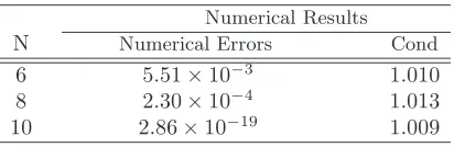
We have reported the results in Table 1. Indeed, Table 1 shows that applying generalized Jacobi polynomials as basis functions in the discrete Galerkin solution of this example concludes very accurate and more reliable results with a suitable degree of approximationN. In addition, we can deduce the stability and wellposedness of the proposed scheme because the condition numbers of resulting discrete Galerkin system are small and independent from approximation degreeN.
Table 1: Numerical results of the Example 1.
Numerical Results
N Numerical Errors Cond
6 5.51×10⁻³ 1.010
8 2.30×10⁻⁴ 1.013
10 2.86×10⁻¹⁹ 1.009
Example 2: Consider the following equation
(
y(4)(x) + (sinx)y′′(x) +exy(x) =f(x) +R I
xty(t)dt,
y(i)(−1) =y(i)(1) = 0, i= 0,1 (4.1)
wheref(x)choose so the exact solution is y(x) = sin4πx.
Here, we compare the results obtained with the proposed discrete Galerkin method with those obtained by a well known pseudospectral method which involves coefficient matrix with large condition numbers and suffers from round off errors whenNtends to infinity. LetD(k) be the kth-order differentiation matrix associated with the
Gauss-Legendre collocation points. Applying Gauss-Gauss-Legendre quadrature formula in the integral term the linear system corresponding to the pseudospectral discretization of the problem becomes
Hj(−1)y= 0, j = 0,1
Hj(1)y= 0, j= 0,1
D(4)+A2D(2)+A1−A0 !
y=f ,
where
A2 := Diag sinx0,sinx1, ...,sinxN,
A1 := Diag ex0
, ex1
, ..., exN,
A0 := na0ij oN
i,j=0, a 0
ij:=xitjwj,
Hj(x) := [H0(j)(x), H (j)
1 (x), ..., H (j) N (x)],
y := [y(x0), y(x1), ..., y(xN)],
f := [f(x0), f(x1), ..., f(xN)].
Here {tj}Nj=0 and {wj}Nj=0 are the Gauss-Legendre quadrature points and
corre-sponding weights respectively. Hi(j)(x) is the jth-derivative of the Lagrange polyno-mials of degreeiassociated with a set of Gauss-Legendre points {xi}Ni=0.
Obviously the pseudospectral solution ˜yN(x) := N P
i=0
y(xi)Hi(x) of (4.1) can be characterized by solving the (N+ 1)×(N+ 1) linear system obtained from restricting of (4.2) to its firstN+ 1 rows and columns.
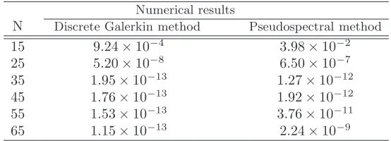
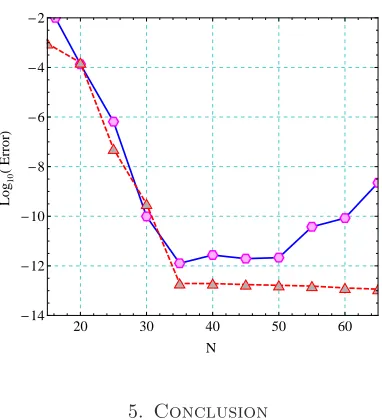
We solve this example by the proposed discrete Galerkin method and the afore-mentioned pseudospectral method and report theL2-errors of them against various N in Table 2 and Figure 1. We observe that the pseudospectral method produces unstable solution for this problem and round off errors destroy the approximation for N >35 while in the discrete Galerkin approach the numerical results are in a good agreement with the exact ones and our method produces an approximate solution with a well-posed and suitable rate of convergence.
Table 2:L2-errors of discrete Galerkin and pseudospectral methods for the Example 2.
Numerical results
N Discrete Galerkin method Pseudospectral method
15 9.24×10⁻⁴ 3.98×10⁻²
25 5.20×10⁻⁸ 6.50×10⁻⁷
35 1.95×10⁻¹³ 1.27×10⁻¹²
45 1.76×10⁻¹³ 1.92×10⁻¹²
55 1.53×10⁻¹³ 3.76×10⁻¹¹
Figure 1. L2-errors versusN when pseudospectral (solid line) and discrete Galerkin (dashed line) methods are used for solving the Ex-ample 2.
20 30 40 50 60
-14 -12 -10 -8 -6 -4 -2
N
Log
10
H
Error
L
5. Conclusion
The discrete Galerkin approximation has been investigated for computing the ap-proximate solution of the higher even-order integro-differential equations with variable coefficients (1.1). It may be concluded that, this methodology is very powerful, well-conditioned in finding numerical solutions for (1.1). In addition the numerical results have been confirmed the efficiency of the proposed scheme.
References
[1] C. Canuto, M. Hussaini, A. Quarteroni, T. Zang, Spectral Methods Fundamentals in Single Domains.Springer-Verlag, Berlin, 2006.
[2] F. Ghoreishi, P. Mokhtary,Spectreal collocation method for multi-order fractional differential equations,Int. J. Comput. Math.,11(2014), no. 5, 1350072, DOI: 10.1142/S0219876213500722 [3] Ben-Yu Guo, Jie Shen, Li-Lian Wang, Optimal Spectral-Galerkin methods using generalized
Jacobi polynomials,J. Sci. Comput.,27(2006), 305–322.
[4] Ben-Yu Guo, Jie Shen, Li-Lian Wang,Generalized Jacobi polynomials/functions and their ap-plications,Appl. Numer. Math.,59(2009), 1011–1028.
[5] J. S. Hesthaven, S. Gottlieb, D. Gottlieb, Spectral Methods for Time-Dependent Problems, Cambridge University Press, 2007.
[6] Majid Khan,A new algorithms for higher order integro-differential equations, Afr. Math.,26 (2015), 247–255.
[7] P. Mokhtary, F. Ghoreishi,Convergence analysis of spectral Tau method for fractional Riccati differential equations,Bull. Iranian Math. Soc.,40(2014), no. 5, 1275–1290.
[9] P. Mokhtary,Reconstruction of exponentially rate of convergence to Legendre-collocation solu-tion of a class of fracsolu-tional integro-differential equasolu-tions,J. Comput. Appl. Math.,279(2014), 145–158.
[10] Xufeng Shang, Danfu Han,Application of the variational iteration method for nth-order integro-differential equations,J. Comput. Appl. Math.,234(2010), no. 5, 1442–1447.
[11] Jie Shen, Tao Tang, Li-Lian Wang,Spectral Methods, Algorithms, Analysis and Applications, Springer, 2011.
[12] Jie Shen,A new Dual-Petrov-Galerkin method for third and higher odd-order differential equa-tions: application to the KDV equation,SIAM J. Numer. Anal.,41(2003), 1595–1619. [13] A. Yildirim,Solving of BVPS for fourth order integro-differential equations by solving Homotopy