Numerical solution of Troesch’s problem using Christov rational
functions
Abbas Saadatmandi∗
Department of Applied Mathematics, Faculty of Mathematical Sciences,
University of Kashan, Kashan 87317-53153, Iran.
E-mail: [email protected]
Tahereh Abdolahi-Niasar
Department of Applied Mathematics, Faculty of Mathematical Sciences,
University of Kashan, Kashan 87317-53153, Iran.
E-mail: [email protected]
Abstract We present a collocation method to obtain the approximate solution of Troesch’s problem which arises in the confinement of a plasma column by radiation pressure and applied physics. By using the Christov rational functions and collocation points, this method transforms Troesch’s problem into a system of nonlinear algebraic equa-tions. The rate of convergence is shown to be exponential. The numerical results obtained by the present method compares favorably with those obtained by various methods earlier in the literature.
Keywords. Troesch’s problem, Christov functions, Collocation, Wiener functions.
2010 Mathematics Subject Classification. 65L60, 41A20.
1. Introduction
The aim of this paper is to introduce a new approach for the numerical solution of the Troesch’s problem. This problem, which is a nonlinear two point boundary-value problem, is given by
y′′=λsinh(λy), 0≤x≤1, (1.1)
subject to the boundary conditions
y(0) = 0, y(1) = 1, (1.2)
whereλ is a positive constant. Troesch’s problem arises from a system of nonlinear ordinary differential equations which occur in an investigation of the confinement of a plasma column by radiation pressure [28]. Also, Troesch’s problem occurs in the
Received: 24 July 2016 ; Accepted: 24 August 2016.
∗Corresponding author.
theory of gas porous electrodes [15]. Roberts and Shipman [23] give the closed form solution to this problem in terms of the Jacobian elliptic function:
y(x) = 2
λsinh
−1
{
y′(0) 2 sc
(
λx|1−1 4y
′(0)2
)}
, (1.3)
wherey′(0) = 2√1−m, and the constantmsatisfies the solution of the transcendental equation
sinh(λ2) √
1−m = sc(λ|m). (1.4)
Here, the Jacobian elliptic function sc(λ|m) is defined by sc(λ|m) = tanϕ, whereϕ, λ
andmare related by the integral
λ= ∫ ϕ
0
1 √
1−msin2θ dθ.
It has been shown thaty(x) has a singularity located at a pole of sc(λ|m) or approx-imately at [23,27]
xs= 1
λln
( 8
y′(0) )
. (1.5)
As pointed by [23], in addition to its intrinsic interest, Troesch’s problem has become something of a test case for methods of solving unstable two-point boundary value problems because of its difficulties.
There are different techniques for solving Troesch’s problem. Temimi [25] proposed a new discontinuous Galerkin finite element method to solve this problem. Chang in [6] used the simple shooting method and in [5] the author applied the variational iteration method for solving Troesch’s problem. Also, a numerical algorithm based on the decomposition method is presented by Deeba et al. [12] for this problem. In [32] the sinc-Galerkin method is used to solve the nonlinear two point boundary value problem with application to Troesch’s equation. Khuri and Sayfy [20] used a finite element approach based on the cubic B-spline collocation method on both a uniform mesh and a piecewise-uniform Shishkin mesh to solve this problem. Moreover, the modified homotopy perturbation technique [14], differential transform method [7], reproducing kernel Hilbert space method [17] and the Jacobi collocation method [13] are employed to solve Troesch’s problem.
In the current investigation, we construct the solution of Troesch’s problem using a different approach. This approach is based on the collocation technique. Our method consists of reducing the problem to the solution of algebraic equations by expanding the required approximate solution as the elements of the Christov rational functions (CRFs) with unknown coefficients. The properties of CRFs are then utilized to evaluate the unknown coefficients.
method. An application of the model is described in Section 5. Also a conclusion is given in Section 6.
2. Properties of the CRFs
Norbert Wiener introduces the complex-valued rational functions [31, page 35]
ρn(x) = 1 √
π
(ix+ 1)n
(ix−1)(n+1), n= 0,1,2, ..., i=
√
−1, (2.1)
as Fourier transforms of the Laguerre functions. Higgins [16] defined it also for nega-tive indicesnand proved its completeness and orthogonality. One way to see this is to make the change of variable [30]
eiθ= 1 +ix
1−ix, i.e. x= tan θ
2,
which maps the entire real line x∈ [−∞,∞] to θ ∈ [−π, π]. The first work which exclusively deals with the basis functions (2.1) appears to come from [10] in 1982. Christov [10] show that this system consists of two real subsequences of odd functions
Sn and even functionsCn, namely
Sn(x) =
ρn(x) +ρ−n−1(x)
i√2 , n= 0,1,2, ..., (2.2)
Cn(x) =ρn(x)−√ρ−n−1(x)
2 , n= 0,1,2, ... . (2.3)
As pointed by [10], both sequences are orthonormal and each member of (2.2) is orthogonal to all members of (2.3); each member of (2.3) is also orthogonal to all members of (2.2). It is worth indicating that,Sn andCn can be defined for negative
nthrough the relations
S−n=Sn and C−n =Cn.
Unlike Hermite and Laguerre sets of functions which behave exponentially at infinity, this system exhibits asymptotic behavior x−1 for the odd sequence andx−2 for the
even one [10]. The Weiner functions applied successfully to time integration of the Benjamin-Ono equation by James and Weideman [18]. The functions Sn and Cn have been employed as forward solvers in the solution of a differential equation on an infinite interval [10], KdV and Kuramoto-Sivashinsky equation [11], fifth order KdV [1], the time dependent problem of interacting 1D solitons [8] and for computing the stationary solutions of Boussinesq equation [9]. We also refer the interested reader to [2–4]. Very recently, Narayan and Hesthaven [21,22] introduced the generalized Wiener rational basis functions and generalized the algebraically-decaying functions of Wiener. Most of the practically important formulae for the functionsSn and Cn are discussed thoroughly in [10] and here an overview of the basic formulation of these functions required for our subsequent development is presented. The odd functions
Sn and even functionsCn can be expressed in an explicit way:
Sn(x) = √
2
π
∑n+1
k=1(−1)
n+k(2n+1 2k−1
)
x2k−1
Cn(x) = √
2
π
∑n+1
k=1(−1)
n+k+1(2n+1 2k−2
)
x2k−2
(x2+ 1)n+1 , n= 0,1,2, ... . (2.5)
Theorem 2.1. For the first and second derivative of the basis functions, the following recurrence relation hold
dSn(x)
dx =
1 2 {
nCn−1(x)−(2n+ 1)Cn(x) + (n+ 1)Cn+1(x)
}
, (2.6)
dCn(x)
dx =
−1 2
{
nSn−1(x)−(2n+ 1)Sn(x) + (n+ 1)Sn+1(x)
}
, (2.7)
d2Sn(x) dx2 =
−1 4
{
(n2−n)Sn−2(x)−4n2Sn−1(x) + (6n2+ 6n+ 2)Sn(x)
−4(n+ 1)2Sn+1(x) + (n2+ 3n+ 2)Sn+2(x)
}
, (2.8)
d2C
n(x)
dx2 =
−1 4
{
(n2−n)Cn−2(x)−4n2Cn−1(x) + (6n2+ 6n+ 2)Cn(x)
−4(n+ 1)2Cn+1(x) + (n2+ 3n+ 2)Cn+2(x)
}
. (2.9)
Proof. The proof is done by direct verification and the detailed proof can be found
in [10].
Theorem 2.2. The functions Sn and Cn can be expressed, by using trigonometric
functions, in an explicit way:
Sn(x) = (−1)n+1
sin(n+ 1)θ+ sin(nθ) √
2 , (2.10)
Cn(x) = (−1)ncos(n+ 1)√θ+ cos(nθ)
2 , (2.11)
wherex= tanθ2 or θ= 2 arctan(x)is a transformation of the independent variable.
Proof. See Ref. [8].
As said in [8,9] any functionf(x) is a periodic function ofθwith period 2π. Now, any localized function off(x) may be expanded as
f(x) = ∞ ∑
n=0
(anCn(x) +bnSn(x)). (2.12)
which in its turn can be rewritten as a Fourier series for the periodic function
f ( tanθ 2 ) = ∞ ∑ n=0 (
an(−1)ncos(n+ 1)√θ+ cos(nθ) 2
+bn(−1)n+1
sin(n+ 1)θ+ sin(nθ) √
2
)
which are known to have exponential convergence. Since, the Fourier series have exponential convergence for periodic functions, then the exponential convergence of
Cn, Sn series follows [9].
3. Solution with CRFs
The basic idea of our method for solving Troesch’s problem on the interval [0,1] is to transform the problem, with a properly selected variable transformation, to the interval (−∞,+∞) and then to solve the transformed problem by the collocation method. Let y(x) be the solution of boundary value problem (1.1)-(1.2). First of all, we reformulate the problem by applying the transformation ˜y(x) =y(x)−xthat makes the boundary conditions become homogeneous. Therefore problem (1.1)-(1.2) reduces to the following boundary value problem
˜
y′′(x) =λsinh(λ(˜y(x) +x)), 0≤x≤1, (3.1)
˜
y(0) = 0, y˜(1) = 0. (3.2)
Now, application of the variable transformation [24]
x=ψ(t) =1 2tanh
(
t
2 )
+1
2, (3.3)
together with the change of notation
u(t) = ˜y(ψ(t)), (3.4)
transforms the problem to
u′′(t)−ψ ′′(t)
ψ′(t)u
′(t) = (ψ′(t))2λsinh(λ(u(t) +ψ(t))), −∞< t <+∞,
(3.5)
subject to the boundary conditions
lim
t→±∞u(t) = 0. (3.6)
Using (3.3) we get
ψ′(t) =ψ(t)(1−ψ(t)), −ψ
′′(t)
ψ′(t) = 2ψ(t)−1. (3.7)
Substituting (3.7) in (3.5) we obtain
u′′(t) + (2ψ(t)−1)u′(t)−(ψ(t))2(1−ψ(t))2λsinh (
λ(u(t) +ψ(t)) )
= 0, (3.8)
We are now ready to solve (3.8) by using CRFs. The approximate solution foru(t) in (3.8) is represented by
u(t)≈uN(t) = N ∑
i=0
It is noted that, the approximate solution in (3.9) satisfies the boundary conditions (3.6) sinceSn(t) and Cn(t) are zero whent→ ±∞. A collocation scheme is defined by substitutinguN(t) into the (3.8) and evaluating the result at
ti= ln ( x
i 1−xi
)
, i= 1,2,· · · ,2N+ 2,
where
xi=ih, i= 1,2,· · ·,2N+ 2, h= 1 2N+ 3. Employing Theorem2.1, forj= 1,2,· · ·2N+ 2, we get
(∑N
i=0
aiCi′′(tj) +biSi′′(tj) )
+ (2ψ(tj)−1) (∑N
i=0
aiCi′(tj) +biSi′(tj) )
−(ψ(tj))2(1−ψ(tj))2λsinh (
λ
((∑N
i=0
aiCi(tj) +biSi(tj) )
+ψ(tj) ))
= 0.
(3.10)
Equation (3.10) generates a set of 2N+ 2 nonlinear algebraic equations, which can be solved for the unknown coefficients{ai}N
i=0 and{bi}Ni=0. Thus,uN(t) given in (3.9) can be calculated. Consequently the unknown function y(x) may be approximated by
yN(x) =uN (
2 tanh−1(2x−1))+x.
Remark 3.1. It is worth to mention here that, the system (3.10) can be solved by applying an iterative method, like the Newton’s method. Having solved the nonlinear system (3.10) analytically for very smallN, sayN = 1, we see that some components of solution of this system are close to zero. Therefore, for larger values of N the initial guesses forai’s and bi’s of the Newton’s method can be estimated by values close to zero. Throughout this paper, we use the Maple’s fsolve command with the initial approximationai=bi= 0.01. Also, we note that the Newton’s method has a convergence rate of quadratic order, which directly depends on the equations of (3.10) and initial guesses forai’s andbi’s.
4. Results and discussion
Table 1. Comparison of absolute error forλ= 0.5.
x Exact Laplace [19] MHPM [14] Spline [20] SGM [32] CRFs (N=9)
0.1 0.095176 7.7×10⁻⁴ 8.2×10⁻⁴ 7.7×10⁻⁴ 7.7×10⁻⁴ 2.1×10⁻⁴ 0.2 0.190633 1.5×10⁻³ 1.6×10⁻³ 1.5×10⁻³ 1.5×10⁻³ 5.8×10⁻⁴ 0.3 0.286653 2.1×10⁻³ 2.3×10⁻³ 2.1×10⁻³ 2.1×10⁻³ 1.2×10⁻³ 0.4 0.383522 2.7×10⁻³ 2.9×10⁻³ 2.7×10⁻³ 2.7×10⁻³ 1.9×10⁻³ 0.5 0.481537 3.0×10⁻³ 3.2×10⁻³ 3.0×10⁻³ 3.0×10⁻³ 2.4×10⁻³
0.6 0.581002 3.1×10⁻³ 3.4×10⁻³ 3.1×10⁻³ 3.1×10⁻³ 2.5×10⁻³
0.7 0.682235 3.0×10⁻³ 3.2×10⁻³ 3.0×10⁻³ 3.0×10⁻³ 2.3×10⁻³
0.8 0.785571 2.4×10⁻³ 2.7×10⁻³ 2.4×10⁻³ 2.4×10⁻³ 1.8×10⁻³
0.9 0.891367 1.5×10⁻³ 1.6×10⁻³ 1.5×10⁻³ 1.5×10⁻³ 9.3×10⁻⁴
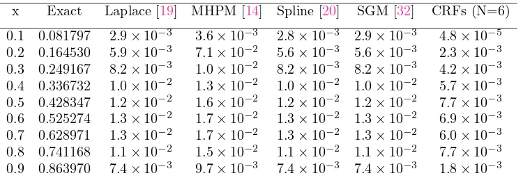
Table 2. Comparison of absolute error forλ= 1.
x Exact Laplace [19] MHPM [14] Spline [20] SGM [32] CRFs (N=6)
0.1 0.081797 2.9×10⁻³ 3.6×10⁻³ 2.8×10⁻³ 2.9×10⁻³ 4.8×10⁻⁵ 0.2 0.164530 5.9×10⁻³ 7.1×10⁻² 5.6×10⁻³ 5.6×10⁻³ 2.3×10⁻³
0.3 0.249167 8.2×10⁻³ 1.0×10⁻² 8.2×10⁻³ 8.2×10⁻³ 4.2×10⁻³
0.4 0.336732 1.0×10⁻² 1.3×10⁻² 1.0×10⁻² 1.0×10⁻² 5.7×10⁻³
0.5 0.428347 1.2×10⁻² 1.6×10⁻² 1.2×10⁻² 1.2×10⁻² 7.7×10⁻³
0.6 0.525274 1.3×10⁻² 1.7×10⁻² 1.3×10⁻² 1.3×10⁻² 6.9×10⁻³
0.7 0.628971 1.3×10⁻² 1.7×10⁻² 1.3×10⁻² 1.3×10⁻² 6.0×10⁻³
0.8 0.741168 1.1×10⁻² 1.5×10⁻² 1.1×10⁻² 1.1×10⁻² 7.7×10⁻³
0.9 0.863970 7.4×10⁻³ 9.7×10⁻³ 7.4×10⁻³ 7.4×10⁻³ 1.8×10⁻³
Figure 1. Comparison of absolute error forλ= 0.5
0 0.1 0.2 0.3 0.4 0.5 0.6 0.7 0.8 0.9 1
0 0.5 1 1.5 2 2.5 3
3.5x 10
−3
x
Absolute error
λ=0.5
Figure 2. Comparison of absolute error forλ= 1
0 0.1 0.2 0.3 0.4 0.5 0.6 0.7 0.8 0.9 1
0 0.002 0.004 0.006 0.008 0.01 0.012 0.014 0.016 0.018
x
λ=1
Laplace Perturbation Spline Sinc−Galerkin CRFs
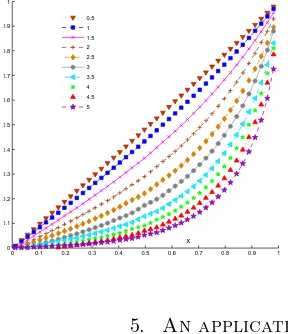
Figure 3. Aproximated solutions of Troesch’s problem by using
CRFs for λ≤5
0 0.1 0.2 0.3 0.4 0.5 0.6 0.7 0.8 0.9 1 0
0.1 0.2 0.3 0.4 0.5 0.6 0.7 0.8 0.9 1
x
0.5 1 1.5 2 2.5 3 3.5 4 4.5 5
5. An application
The plasma will be regarded as consisting of two oppositely charged ideal gases which penetrate each other without friction. The Troesch’s problem which arises in the investigation of the confinement of a plasma column by radiation pressure, was initially introduced and formulated by Weibel and Landshoff [29] and Troesch [26]. In this section we will trace its origin to a system of ordinary differential equations derived and solved in natural units [26,29].
1
r d dr(r
dE0 dr ) +
(
ω2−e 2N
M −
e2n m
)
E0= 0, (5.1)
1
r d
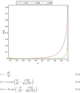
Figure 4. Aproximated solutions of Troesch’s problem by using
CRFs for λ >5
Er=−
dU
dr, (5.3)
n(r) =n0exp
(
eU kT −
e2E2 0
4mω2kT
)
, (5.4)
N(r) =N0exp
( −eU
kT − e2E2
0
4M ω2kT
)
, (5.5)
where n and N are variable ion and electron densities, E = (Er(r),0, E0(r) cosωt)
is the electric field andE0(r) cosωtrepresents the applied field plus the field due to
the plasma current. Also,T is temperature and equation (5.3) represents the radial electrostatic field due to charge separation. Moreover, Ion and electron temperatures are assumed equal and constant.
As described in [26], if these equations are considered in Cartesian, rather than polar coordinates, and if,E0 is assumed to be negligibly small, then the system reduces to
dE
E(x) =−dU
dx, (5.7)
n(x) =n0exp(λU), (5.8)
N(x) =N0exp(−λU), (5.9)
up to constant factors. Substituting (5.7),(5.8) and (5.9) into (5.6), a second-order nonlinear ordinary differential equation is obtained as
d2U
dx2 =N0exp(−λU)−n0exp(λU). (5.10)
Also, applying the simplifying assumptionN0 =n0 = N∗ and setting U = −y, we
can write
y′′= 2N∗sinh(λy). (5.11)
6. Conclusion
In this study, a new method using the Christov rational functions, to numerically solve the Troesch’s problem is presented. The comparison of the results obtained by the present method, the exact solution and the other methods reveals that the method is very effective and convenient. The work emphasized our belief that the method is a reliable technique to handle these types of problems.
References
[1] K.L. Bekyarovc, C.I. Christov, Fourier-Galerkin numerical technique for solitary waves of fifth order Korteweg-de Vries equation,Chaos, Solitons and Fractals,1(5) (1991), 423-430. [2] J.P. Boyd, The orthogonal rational functions of Higgins and Christov and algebraically mapped
Chebyshev polynomials,Journal of Approximation Theory,61 (1990), 98-105.
[3] J.P. Boyd, Z. Xu, Comparison of three spectral methods for the Benjamin-Ono equation: Fourier pseudospectral, rational Christov functions and Gaussian radial basis functions,Wave Motion,
48 (2011) 702-706.
[4] J.P. Boyd, Z. Xu, Numerical and perturbative computations of solitary waves of the Benjamin-Ono equation with higher order nonlinearity using Christov rational basis functions,Journal of Computational Physics231 (2012), 1216-1229.
[5] S.H. Chang, A variational iteration method for solving Troesch’s problem,Journal of Compu-tational and Applied Mathematics, 234 (2010), 3043-3047.
[6] S.H. Chang, Numerical solution of Troesch’s problem by simple shooting method,Applied Math-ematics and Computation, 216 (2010), 3303-3306.
[7] S.H. Chang, I.L. Chang, A new algorithm for calculating one-dimensional differential transform of nonlinear functions,Applied Mathematics and Computation, 195 (2008), 799-808.
[8] M.A. Christou, C.I. Christov, Interacting localized waves for the regularized long wave equation via a Galerkin spectral method,Mathematics and Computers in Simulation,69 (2005), 257-268. [9] M.A. Christou, C.I. Christov, Fourier-Galerkin method for 2D solitons of Boussinesq equation,
Mathematics and Computers in Simulation,74 (2007), 82-92.
[10] C.I. Christov, A complete orthonormal system of functions inL2(−∞,∞) space,SIAM Journal
of Applied Mathematics, 42(6) (1982), 1337-1344.
[12] E. Deeba, S.A. Khur, S. Xie, An algorithm for solving boundary value problems, Journal of Computational Physics, 159 (2000), 125-138.
[13] E.H. Doha, D. Baleanu, A.H. Bhrawy, R.M. Hafez, A Jacobi collocation method for troesch’s problem in plasma physics,Proceedings of the Romanian Academy-Series A, 15 (2014), 130-138. [14] X. Feng, L. Mei, G. He, An efficient algorithm for solving Troesch’s problem, Applied
Mathe-matics and Computation, 189 (2007), 500-507.
[15] D. Gidaspow, B.S. Baker, A model for discharge of storage batteries, Journal of The Electro-chemical Society, 120 (1973), 1005-1010.
[16] J.R. Higgins,Completeness and basis functions of sets of special functions, Cambridge Univer-sity Press, Cambridge, 1977.
[17] M. Inc, A.Akg¨ul, The reproducing kernel Hilbert space method for solving Troesch’s problem,
Journal of the Association of Arab Universities for Basic and Applied Sciences, 14 (2013), 19-27.
[18] R.L. James, J.A.C. Weideman, Pseudospectral methods for the Benjamin-Ono equation, in: R. Vichnevetsky, D. Knight, G. Richter (Eds.), Advances in Computer Methods for Partial Difierential Equations,7 (1992), 371-377.
[19] S.A. Khuri, A numerical algorithm for solving the Troesch’s problem, International Journal of Computer Mathematics, 80 (2003), 493-498.
[20] S.A. Khuri, A. Sayfy, Troesch’s problem: A B-spline collocation approach, Mathematical and Computer Modelling, 54 (2011), 1907-1918.
[21] A.C. Narayan, J.S. Hesthaven, A generalization of the Wiener rational basis functions on infinite intervals: part I - derivation and properties,Mathematics of Computation, 80 (2011), 1557-1583. [22] A.C. Narayan, J.S. Hesthaven, A generalization of the Wiener rational basis functions on infinite intervals: Part II - numerical investigation,Journal of Computational and Applied Mathematics, 237 (2013), 18-34.
[23] S.M. Roberts, J.S. Shipman, On the closed form solution of Troesch’s problem, Journal of Computational Physics, 21 (1976), 291-304.
[24] M. Sugihara, Double exponential transformation in the Sinc-collocation method for two-point boundary value problems,Computational and Applied Mathematics,149(2002), 239-250. [25] H. Temimi, A discontinuous Galerkin finite element method for solving the Troesch’s problem,
Applied Mathematics and Computation, 219 (2012), 521–529.
[26] B.A. Troesch, A Simple Approach to a Sensitive Two-Point Boundary Value Problem, Journal of Computational Physics, 21 (1976), 279-290.
[27] B.A. Troesch,Intrinsic difficulties in the numerical solution of a boundary value problem, In-ternal Report NN-142, TRW Inc., Redondo Beach, California, 1960.
[28] E.S. Weibel,On the confinement of a plasma by magnetostatic fields,Phys. Fluids,2(1) (1959), 52-56.
[29] E.S. Weibel, R.K.M. Landshoff, The Plasma in Magnetic Field, Stanford University Press, Stanford, 1958.
[30] J.A.C. Weideman, Computing the Hilbert transform on the real line, Mathematics of Compu-tation, 64 (1995), 745-762.
[31] N. Wiener,Extrapolation, interpolation, and smoothing of stationary time series, MIT Tech-nology Press and John Wiley and Sons, New York, 1949.