AUT J. Model. Simul., 50(2) (2018) 203-210 DOI: 10.22060/miscj.2018.13961.5087
Global Stabilization of Attitude Dynamics;
SDRE-based Control Designs
M. Safi1, M. Mortazavi2*, S. M. Dibaji3
1 Hardware In the Loop Laboratory, Department of Aerospace Engineering, Amirkabir University of Technology, Tehran, Iran
2 Centre of Excellence in Computational Aerospace, Department of Aerospace Engineering, Amirkabir University of Technology, Tehran, Iran 3 Active-Adaptive Control Lab, Massachusetts Institute of Technology, Cambridge, MA, USA
ABSTRACT: The State-Dependant Riccati Equation method has been frequently used to design suboptimal controllers applied to nonlinear dynamic systems. Different methods for local stability analysis of SDRE controlled systems of order higher than two such as the attitude dynamics of a general rigid body have been developed in the literature; however, it is still difficult to show global stability properties of closed-loop system with this controller. In this paper, a reduced-form of SDRE formulation for attitude dynamics of a general rigid body is achieved by using Input-State Linearization technique and solved analytically. By using the solution matrix of the reduced-form SDRE in properly defined Lyapunov functions, a class of nonlinear controllers with global stability properties is developed. Numerical simulations are performed to study the stability properties and optimality for attitude stabilization of a general rigid body, and it is concluded that the designed controllers have the capability to provide a balance between optimality and proper stability characteristics.
Review History: Received: 14 January 2018 Revised: 24 October 2018 Accepted: 27 November 2018 Available Online: 5 December 2018 Keywords:
SDRE Lyapunov
Exponential Stability Global Stability Attitude Dynamics 1- Introduction
Numerous techniques exist to design control laws for nonlinear systems such as gain scheduling, feedback linearization, sliding mode control, backstepping and adaptive control. Each of these techniques has its own tuning methods which allow the designer to provide trade-offs between different factors such as control effort and output error. Also, features like robustness to uncertainties and disturbances as well as stability issues depend on the controller design.
State-Dependent Riccati Equation (so-called SDRE) is a well-known systematic and effective technique which has been widely used to design suboptimal controllers, observers, and filters [1]. The SDRE controlled systems are not such restrictive in form as is the case with other control methods like backstepping. Moreover, the most important advantage of SDRE method is its flexibility in tuning the corresponding weighting matrices, as functions of the states, which provide capability of designing adaptive control laws. SDRE-based controllers have been applied to a diverse range of nonlinear systems including the attitude dynamics of rigid bodies (e.g. [2], [3], [4] and [5]). In all such applications, the resulting closed-loop system is locally asymptotically stable and the global stability properties cannot be determined because the SDRE controlled system is not known in closed-form. A global stability analysis for second-order systems under SDRE control has been investigated in [6], where the system’s equations are parameterized so as to yield an analytical solution to the SDRE. However, for a system with state dimension higher than two, it is still difficult to achieve an analytical solution to the SDRE, although, there exist some methods to calculate the region of attraction of
closed-loop system [7]. Moreover, using the Euler angles as attitude feedbacks usually causes singularities in the solution. On the other hand, all pure SDRE attitude controllers that use quaternion vector part as feedback encounter uncontrollability when they want to stabilize the largest attitude maneuver, i.e. the initial error angle is taken as 180 degrees (see, e.g. [8] and [9]).
To address the aforementioned concerns, here we provide a novel approach by combining SDRE, Input-State Linearization (ISL), and Lyapunov method. We use ISL technique to partly simplify the rigid body attitude dynamics. Implementing some mathematical operations make it possible to find an analytic solution for the obtained simplified SDRE. By using the solution matrix of the reduced-form SDRE in properly defined Lyapunov functions, a new class of nonlinear controllers with global stability properties is developed. Indeed, this approach provides a trade-off between stability properties and optimality for attitude stabilization of a rigid body. This class of controllers has also no uncontrollability pitfall. Due to the nature of the quaternion parameters, which are used for representation of attitude kinematics, the presented solution and consequently the controllers are globally non-singular. This feature is very important in the attitude stabilization problem.
through some numerical examples in Section 5. Finally, Section 6 concludes the paper.
2- Preliminaries And Background 2- 1- Attitude Dynamics Equations
Euler’s equation describes the attitude dynamics of a rigid body around body-fixed axes with origin at the center of mass. The following equation is associated with the general case, where the body-fixed control axes do not coincide with the principal axes of inertia.
- ,
Jω = u S Jω ω (1)
where
[
1 2 3]
T
ω= ω ω ω is the body angular velocity with respect to an inertial coordinate,
[
1 2 3]
T
u= u u u is the control torque vector, J indicates the inertial matrix, and Sω
represents a skew-symmetric matrix defined as
3 2 3 1 2 1 0 0 0 Sω −ω ω = ω −ω −ω ω .
The subscripts 1, 2 and 3 denote the body-fixed control axes. 2- 2- Attitude Kinematics Equations
Attitude of a rigid body can be described by different methods with their special properties [10]. However, for sake of simplicity, quaternion representation, which is globally non-singular, is preferred to design attitude controller
(
)
1 , 2 1 , 2 T Sε ε = ηω + ω η = ω ε (2)where
[
1 2 3]
T
ε = ε ε ε is the vector part of quaternion, η is its scalar part, and Sε is a skew-symmetric matrix defined by
3 2 3 1 2 1 0 0 , 0 Sω ω ω ω ω ω ω − = − − (3)
where the quaternion parameters satisfy the quaternion
2 T 1.
η + ε ε = (4)
Rigid body stabilization problem is achieved by the stabilization of the two equilibrium points (ε =0,η = ±1,
0
ω = ) of the dynamics defined by and . This duality of the quaternion parameters is because of their nature in attitude representation [10]. Briefly, note that unit quaternions are used to parameterize SO
( )
3 which is a boundary-less compact manifold for representation of rigid body attitude. The state space of quaternions, 3(the set of unit-magnitude vectors in 4) is also a boundary-less compact manifold that provides a double covering of SO( )
3 where always two sets of unit quaternions correspond to a single attitude (see [11] for details).2- 3- Review of SDRE Control Method
Consider the general infinite-horizon regulation problem, where the system is fully observable and affine in the input and represented in the form of
( )
( )
x f x = +g x u
(5)
where x∈n, u∈m, f x
( )
and g x( )
are smooth, and( )
0. x g x∀ ≠ It is desired to find a state feedback control law u x
( )
which regulates the system to the origin ∀x and minimizes the performance index( ) ( )
(
)
0
1
2 x Q x x u R x u dtT T
∞
Φ =
∫
+where Q x
( )
and R x( )
are the state and control weighting matrices, respectively. The SDRE method approaches the problem by mimicking the LQR formulation for linear systems. Accordingly, the system equation (5) is first written in the linear-like structure( )
( )
x A x x B x u= + (6)
where f x
( )
=A x x( )
and g x( )
=B x( )
. According to [12], this factorization is not unique and is possible if and only if( )
0 0f = and f x
( )
is continuous.Lemma 1. Consider (6)and the following conditions. i. The full-state measurement vector is available. ii. f x
( )
is continuously differentiable and f( )
0 =0. iii. g x( ) is smooth and ∀ x g x( )
≠0.iv. Q x
( )
and R x( )
are positive definite.v. ∀x the pair
(
A x B x( ) ( )
,)
is point-wise controllable. Then, the suboptimal state-feedback control law is obtained in the form of( )
( )
( ) ( ) ( )
1 T
u x K x x
R− x B x P x x
= −
= − (7)
where P x
( )
is the unique, symmetric, positive-definite solution of the state-dependent algebraic Riccati equation( ) ( )
( ) ( )
( )
( ) ( )
1( ) ( ) ( )
0.T
T
A x P x P x A x Q x
P x B x R− x B x P x
+ +
− = (8)
The reader can refer to [12] for the detailed proofs. 2- 4- Full SDRE Controller of Rigid Body Attiude 2- 4- 1- State-Dependant Factorization
Equation (1) and first line of(2) are used to form the state-space equations. The angular velocity vector and the quaternion vector part are defined as states of the system. According to (5), and if we construct T T T
x= ω ε , then we have
( ) ( ) ( ) 1 1 , , 1 0 2
J S J J
f x g x
S − − ω ε − ω = = ηω + ω
where I∈3 3× is an identity matrix (all over the paper),
( )
f x is continuous with f
( )
0 =0. Therefore, the state-dependent factorization is possible and can be configured in the following form, (the argument x is dropped for simplicity in the rest of the paper)1 1
1 1
0 ,
0 0
0 ,
J S J J u
A
u R J P
− − ω ε − − ω − ω = + ε ε ω = − ε (9)
where with regard to (6), A and B can be defined. Also, from(2) and (3), Aε is represented by
Note that the quaternion scalar part η that appears in the above matrix can be calculated from quaternion vector part as stated in (4):
1 T .
η = ± − ε ε
The process of selecting quaternion to use for feedback is not obvious. Two options are presented here to avoid ambiguity of quaternion scalar part if the tracking problem is considered. First, the assumption of η ≥0 is taken [4]. Second, choosing the sign of quaternion at the current time step to agree with the commanded attitude at the previous time step such that
( ) ( ) ( ) ( )
1 1 0, Tk k k k
t − t t − t
ε ε + η η > for k >1 [13]. The second option forces a condition to achieve an analytic solution to the reduced SDRE which will be discussed later where the closed-form solution is presented. Moreover, a simple hybrid-dynamic algorithm for path lifting from SO
( )
3 to 3 is presented in [14] which addresses the mentioned ambiguity issue.2- 4- 2- Controllability Analysis
Here, we show that the closed-loop system (9) is controllable.
Proposition 1. For all η ≠0, system (9) is point-wise controllable.
Proof. According to [12], a sufficient condition for
controllability of the system (9) can be achieved by checking that the controllability matrix constructed by the pair
(
A B,)
is full rank. Controllability matrix of the pair
(
A B,)
isformed as:
( )
( )
5 , 11 1 1
1 1, ,5 1 A B k k k k k
C B AB A B
J S
A B k
A J S
ω ε ω − − − − = − ℵ⊕⊕ℵ −
Note that A B A Bk k+1 =0 if k =1, ,4
; thus, CA B, cannot be a full rank matrix based on its last five blocks. Instead, the determinant of the first two blocks is calculated as below:
2 1 8 J
B AB η
−
=
The above determinant is nonzero while η ≠0. Thus, the system (9) is, for all η≠0, point-wise controllable.
Remark 1. In regulation problem, the system cannot be stabilized by the “Full SDRE” controller when the initial Euler angle between body-fixed and reference coordinate axes (E =2cos−1η) is exactly180 deg.
3- Combination of SDRE with ISL 3- 1- Reduction of SDRE
ISL is one of the feedback linearization techniques which are used to design controllers for a class of nonlinear systems. Here, ISL technique is just applied to the dynamical equation and simplifies the mathematical model using the following Lemma.
Lemma 2. Consider the problem of designing the control input u in (5). The affine system (5) is input-state linearizable and the transformed system and its control input are ω = v and u Jv S J= + ω ω respectively.
Proof. An affine system is input-state linearizable if a
state transformation z z x=
( )
and an input transformation(
,)
u u x v= are found so that the nonlinear system dynamics is transformed into an equivalent LTI dynamics, in the
companion form z az bv= + . System (1) is affine and we take the state and input transformations as it follows.
z
u Jv S Jω = ω
= + ω (10)
Then, the attitude’s dynamical equation can be simplified to the companion form:
. v
ω =
This completes the proof.
Now, we can obtain v by the SDRE method as the transformed dynamical system is in LTI form. Accordingly, overall system (1) is stabilized with input transformation v. According to (5), we have:
(
)
0 , , 1 0 2 I f g Sε = = ηω + ω where I is an identity matrix with order three (all over the paper), f is continuous while f
( )
0 =0. Therefore, referring to Lemma 1, the state-dependent factorization is possible and can be configured in the form of0 0 . 0 0 I v Aε ω ω = + ε ε (11)
Referring to (6), we can redefine A and B in (11). Similar to the previous case, controllability of the above system can be analyzed.
Proposition 2. For any η ≠0, the reduced-form system as in (11) is point-wise controllable.
Proof. According to new pair
(
A B,)
, it is easily revealed that Ak =06 6× =k 2, ,5 . Therefore, we have:[
]
, 06 12 .
A B
C = B AB × (12)
Similar to Proposition 1, to see whether CA B, is full rank, it is sufficient to examine its two first blocks. These two blocks together are square matrix with order six which is full rank if and only if its determinant is nonzero. Substituting AandB
in , the determinant is calculated as follows: 1
8
B AB = η
Thus, the system(11) is, for all η ≠0, point-wise controllable. The above Proposition states a sufficient condition for controllability of the system (1) . In Section 4, a necessary and sufficient condition is proposed where the equilibrium of the system becomes globally asymptotically stable with the proposed controllers.
3- 2- Analytic Solution of the Reduced-form SDRE
Theorem 1. Assume that Q and R are strictly positive definite diagonal matrices in the form of:
( )
1 2 2 1 1 2 2 2 2 0 0 , 1,2,3 , , i Q Q QQ diag q i
Q q I R r I
= = = = = (13)
where q q1i, 2 and r are arbitrary positive real numbers and
( )
Proof. If the block matrix P , that is the solution of SDRE associated to equation (11), defined as:
1 2
3 4
,
P P P
P P
=
(14)
according to Lemma 1 and basic mathematical properties of block matrices, we can conclude that i) P1 to P4 are unique square matrices with order three, ii) P2 and P3 are not necessarily positive definite but P3 =P2T and iii) P1 and
4
P are symmetric positive definite matrices. Using (11) and substituting of(13) and (14) into , (8) it holds that:
2
2 2 2 1 1
4 2 1 2 4 2 2 1 2 2 2 2
1 0,
1 0,
1 0,
1 0.
T T
T T
A P P A P Q
r
A P PP
r P A P P
r
Q P P
r
ε ε
ε
ε
+ − + =
− =
− =
− =
(15)
Using Lemma 2, we obtain the transformed system (11). Then, substituting (13) in (7), the state feedback control v
can be achieved by
(
1 2)
1 .
2
v = − Pω + εP (16)
Thus, only P1and P2must be known. Let us discuss the solution of P2 at first. The fourth line of equation (15) can be transformed into the form
2 2T 2 2 P P =r Q ,
which can be satisfied by
2 2
P = λrq I (17)
where λ = ±1is the sign of P2. Here, we choose λ = +1. In Theorem 2, we will clarify its reason.
Next, on the basis of known P2, the solution for P1 is followed. The first line of equation (15) can be transformed as:
(
)
2 2
1 T 2 2 1 .
P =r A P P A Qε + ε+ (18)
According to (17) and knowing positive definiteness of P1, by obtaining the square root of both sides of(18) we obtain:
(
2)
1 1i 2 , 1,2,3.
P diag r q= +rqη =i (19)
Knowing positive definiteness of weighting matrices, P1 in (19) can be the solution of(18) under one of the following conditions: i) the assumption η ≥0 is satisfied. Then, all the components under the radicals are positive real numbers. ii) The sign of η is arbitrary. Then, the weighting matrices need to be selected carefully. Since the quaternion norm is bounded, the sufficient condition 2
1i 2 1,2,3
q ≥rq i = has to be satisfied. This completes the proof.
4- Stability Analysis of Closed Loop System
In this section, Lyapunov direct method along with LaSalle’s theorem are used to confirm the solution of SDRE derived in Section 3 and also to ensure the globally asymptotic stability of the overall closed-loop system. Note that stability analysis in the unit-quaternion space 3 is related to a corresponding one in the SO
( )
3 state space that will be addressed in [14].4- 1- Globally Asymptotic Stability of Closed Loop System Substituting (16) into (10), the following control law is obtained:
(
1 2)
2
1 ,
SDRE ISL
u J P P S J
r
+ = − ω + ε + ω ω (20)
where P1 and P2 can be obtained from (19) and (17), respectively.
Theorem 2. The control law (20) makes the equilibrium of the overall closed-loop system (1) globally asymptotically stable (even in η =0).
Proof. First, we apply (20) to the original dynamics system (1) which makes it equivalent to the closed-loop system (11). For simplicity, we consider stability analysis of system (11) instead (the cross-coupling term will be omitted when we derive V). Substituting (16) into (11), the closed-loop system of (11) is:
(
1 2)
1 ,
2 P P
ω = − ω + ε (21)
where only the attitude’s dynamical equation is concerned. Choose the candidate Lyapunov function
(
)
22 1
2
1 1 ,
2
T T
V = r ω P−ω + ε ε + − η (22)
which is positive definite and radially unbounded, i.e. limω→∞V = ∞. From (2),(3), (21), the time derivative of (22) is calculated as (note that 1
2
P− is a symmetric matrix)
1 2 1 ,
T
V = −ω P P− ω (23)
where V< ∀ω ≠ 0, 0 , and V=0 if ω =0. Thus, using the LaSalle’s theorem [15], globally asymptotic stability (GAS) of the closed-loop system (11), and accordingly overall system (1), is proved. Note that P1 is positive definite. Thus, referring to (23), 1
2
P− needs to be positive definite. Then,
the assumption of λ = +1 (in Theorem 1) is confirmed. This completes the proof.
Remark 2. Note that Theorem 2 provides a necessary and sufficient condition for controllability of the overall closed-loop system . Therefore, the uncontrollability of reduced SDRE in η =0 is relaxed.
It is noteworthy that if we omit the angular velocity cross-coupling, the following control law can be designed,
(
)
ReducedSDRE 12 1 2 ,
u = − Pω + P ε (24)
where calculates the Euclidean norm of its input. Indeed, controller (24) is the well-known PD controller with quaternion feedback [16]. However, we use the solution matrix of the reduced SDRE instead of classical gains here.
Proposition 3. The control law (24) makes the equilibrium of the overall closed-loop system (1) globally asymptotically stable.
Proof. Consider the candidate Lyapunov function:
(
)
(
2)
2
2
1 1 ,
2 T T
V = r ω ω +J P ε ε + − η (25) which is positive definite and radially unbounded.
0
TS J
ω
ω ω = , time derivative of (25) becomes
1 . T V= −ω Pω
As P1 is positive definite, we have V < ∀ω ≠0 0 and V=0 for ω =0. Using the LaSalle’s invariance principle, GAS of the closed-loop system and is proved.
Remark 3. With the control law (24), the overall closed-loop system (1) is globally asymptotically stable without knowing the moments of inertia matrix. It is a desirable feature in practice.
4- 2- Global Exponential Stability of Closed Loop System If we add the derivative of the vector part of quaternion parameters as a feedback, the controller v can be designed as follows:
1 2 1
2 2 2
P P PG
v G
r r r
= − ω − ε − ε − ε
where G is a positive definite diagonal matrix. Then, using ISL technique and returning to (1), the following control law is achieved (note that ε is a function of ε ω η, , ):
(
2 1)
21 1
2 2 2 .
SDRE ISL LY P J
u P PG
r GS P G
J J S J
r + +
− ε
ω
= − + ε
− + η + − ω
(26)
Theorem 3. The control law (26) makes the equilibrium of the closed-loop system(1) globally exponentially stable. Proof. Consider a candidate Lyapunov function as
(
)
(
)
(
)
2
2 1
2 1
2
T T
r
V = ω + εG P− ω + ε + ε ε + − ηG
which is positive definite and radially unbounded. With some simplifications the time derivation of the above function is derived as:
(
)
1(
)
2 1
T T
V= − ω + εG P P− ω + ε − εG Gε
As a result, GAS of the closed-loop system is achieved using the Lyapunov direct method (similar to the proof of Theorem 2). Note that ω + ε →G 0 and ε →0 implies that ω →0 . Also, according to , we have η → ±1. Now, to prove the Global Exponential Stability (GES), we use equation (4) where ε = − η ≥ − η2 1 2 1 (note that η = −1 is excluded for angles less than 180 deg such that 0≤ ≤η 1). Therefore, V
can be bounded as follows:
( )
{
}
(
)
1 2 max 2
2 2
max 2, 2
.
V P r
G
−
≤ λ ×
ε + ω + ε (27)
On the other hand, V can be bounded as:
( )
(
)
{
}
(
)
1
min min 2 1
2 2
min ,
.
V G P P
G
−
≤ − λ λ ×
ε + ω + ε
(28)
Hence, from (27) and (28), we can conclude that V≤ −αV, where α is the minimum convergence rate of the rigid body dynamics’ system and is formed by the gain matrices as it follows:
( )
(
)
{
}
( )
{
}
1
min min 2 1
1 2 max 2
min ,
,
max 2, 2
G P P
P r
−
−
λ λ
α =
λ (29)
where λminand λmaxdenote the minimum and maximum eigenvalue of the input matrix, respectively.
Consider the controller (26) and the expression of minimum convergence rate obtained in (29). If r q= 2=q, 2
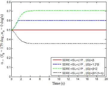
1i q =β q and G =β 2 ,I then the system’s minimum convergence rate becomes α = β 1+ η 2. Thus, with η →1, α→β 2 2. This means as the system converges to the equilibrium point the minimum convergence rate is increasing. The rate becomes decreasing and tends to β 2 4 if G =β 1+ηI. Indeed, the minimum convergence rate of the closed-loop system with “SDRE+ISL+LYP” control law can be tuned easily to any arbitrary amount by appropriate selection of gain matrix G and weighting matrices Q and R.
5- Numerical Simulations
In this section, a sample attitude maneuver of a general rigid body using designed controllers is simulated. Also, further discussions are presented to study the stability and optimality properties of the closed-loop system using numerical simulations.
5- 1- Sample Attitude Maneuver
First, we define constants, initial conditions and weighting matrices. Principle and cross product elements of inertial moments’ matrix are taken asJp =2 and Jcp =0.2 , respectively. Also, weighting matrices are chosen as
3
1 2 5 10 .
Q Q= =R = × I
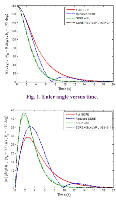
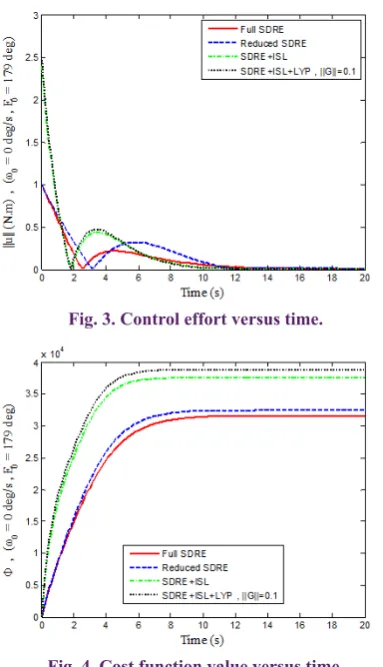
Fig. 1. Euler angle versus time.
Time history of Euler angle, angular velocity norm, control vector norm and cost function for a sample maneuver with initial angular velocity of ω = 0 0 deg/s and initial Euler angle of E0=179 degare presented in Fig. 1 to Fig. 4, respectively. This fact that the convergence rate opposes the optimality is shown. Note that the “Full SDRE” controller fails with initial Euler angle of E0 =180 deg or η =0. Thus, we consider maneuvers with E0=179 deg in further results such that we can compare all four controllers in terms of optimality. However, global stability of the closed-loop system with the proposed controllers is illustrated in Fig. 12 where the initial angle is set to E0=180 deg.
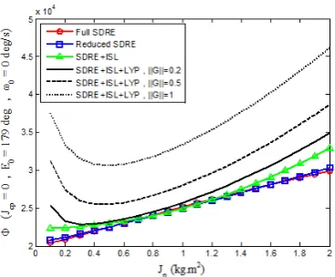
5- 2- Optimality and Stability Properties of Controllers Cost function Φ takes different amounts in presence
of each controller during a definite attitude maneuver. Various moments of inertia matrices and the range of initial conditions, including angular velocity and Euler angle, are other parameters which affect the cost function value. To avoid
ambiguity and make the optimality analysis understandable, effect of each parameter is studied separately. Therefore, we define two maneuver sets to analyze the sensitivity of cost function to each parameter for the proposed controllers versus “Full SDRE” controller. The first maneuver (MS1) starts with initial angular velocity of ω = 0 0 deg sec and initial Euler angle of E0= →0 179 deg. The second maneuver (MS2) starts with initial Euler angle of E0= 0 deg and initial angular velocity norm ω0 =0 → 100 deg sec. Note that the sensitivity of cost function value to principle and cross product inertial moments is analyzed separately. Thus, choose
0
cp
J = to analyze the sensitivity of cost function value to initial conditions and principle moments of inertia. Weighting matrices have been taken the same as sample maneuver.
Table 1. Stability And Optimality Properties Of Closed-Loop System With Presented Controllers
Controller Stability Type Optimality Control-lability Convergence Minimum Rate
Full SDRE LAS Strong Uncontrol-lable in η = 0 -Reduced
SDRE GAS
Almost equivalent
to Full GPC
-SDRE+ISL GAS
SDRE* Lower but
close to Full SDRE
GPC
-SDRE+ISL +LYP GES
Tunable up to
SDRE+ISL GPC Tunable *Even better in some cases
According to Fig. 5 and Fig. 6, cost functions have very close values with small initial conditions for all four methods. The cost function of ”Reduced SDRE” method has almost equal or even less values against the ”Full SDRE” method in both maneuver sets and also with various magnitudes of principle
inertial moments. Besides, Fig. 5 to Fig. 8 show that if G→0,
then response of the dynamic system to “SDRE+ISL+LYP” control attends to the response to “SDRE+ISL” control. Moreover, “SDRE+ISL” and “Reduced SDRE” controllers
have same effects on the dynamic system when J→I.
However, as illustrated in Fig. 7 and Fig. 8, all the cost functions’ values of different control methods are extremely close in a region where the moments of inertia matrix equals to identity.
To consider the sensitivity of cost function to cross product elements of moments of inertia matrix, we define
Table 2. Effects Of Designed Controllers With Respect To Full SDRE On Cost Function Value
Controller Maximum Sensitivity to InitialConditions (%) Maximum Sensitivity to Jp (%) Maximum Sensitivity to σ (%)
MS1 MS2 Ave. MS1 MS2 Ave. MS1 MS2 Ave.
Reduced
SDRE 1.7 -9.5 -5.6 1.7 -6.3 -4 4.4 -12 -8.2
SDRE+ISL 10 13.5 11.7 10 12.5 11.3 31 42 36.5
SDRE+ISL Tunable up to SDRE+ISL
Fig. 3. Control effort versus time.
100.
cp p J J
σ = × As illustrated in Fig. 9 and Fig. 10, the cost function values are more sensitive to cross product elements of inertial moments’ matrix than to the other parameters. In Fig. 11, the conclusions under Theorem 4 are numerically verified for β =1 with the sample attitude maneuver.
All the above discussions on stability properties from Section 4 and optimality are summarized in Table 1. Note that ”GPC” and ”LAS”, respectively, stand for Global Pointwise Controllability and Local Asymptotic Stability. Maximum sensitivity of cost function value with the designed controllers to initial conditions, Jp and σ are numerically stated for both
maneuver sets in Table 2.
It can be concluded that the optimality of “Reduced SDRE”
controller is better than “Full SDRE” controller in all cases in general. Furthermore, optimality difference of other two designed controllers with respect to “Full SDRE” is not egregious. Therefore, we can wisely use the designed SDRE-based controllers along with the “Full SDRE” controller with a trade-off between their optimality and proper stability characteristics.
6- Conclusions
Based on analytic solution of a reduced-form of SDRE for general attitude dynamics, a class of nonlinear suboptimal controllers is presented. Numerical simulations and discussions on stability and optimality properties revealed that the designed controllers inherit the optimality Fig. 5. Cost sensitivity to initial conditions, MS1 Fig. 8. Cost sensitivity to initial conditions, MS2.
Fig. 7. Cost sensitivity to initial conditions, MS2. Fig. 6. Picture Cost sensitivity to initial conditions, MS2
characteristics of the “Full SDRE” controller while having global stability properties. Moreover, the designed control laws are closed-form and globally non-singular. Also, in the “SDRE+ISL+LYP” control law, the minimum convergence rate of the closed-loop system can be tuned just by simply changing the SDRE weighting matrices that is useful in practice. For future works, inspired by the proposed approach one can design controllers for any system which includes attitude dynamics such as quadrotor robots, satellites and robot manipulators. Besides, robustness and adaptiveness of the proposed SDRE-based control laws can be considered in further investigations.
References
[1] J.R. Cloutier, State-dependent Riccati equation techniques: an overview, in: Proceedings of American Control Conference, 1997, pp. 932-936.
[2] H. Voos, Nonlinear state-dependent Riccati equation control of a quadrotor UAV, in: IEEE International Conference on Control Applications, 2006, pp. 2547-2552.
[3] P. Shankar, R. Yedavalli, D. Doman, Dynamic inversion via state dependent Riccati equation approach: Application to flight vehicles, in: AIAA Guidance, Navigation, and Control Conference and Exhibit, 2003, pp. 5361.
[4] M. Abdelrahman, I. Chang, S.-Y. Park, Magnetic torque attitude control of a satellite using the state-dependent Riccati equation technique, International Journal of Non-Linear Mechanics, 46(5) (2011) 758-771.
[5] A. Bogdanov, M. Carlsson, G. Harvey, J. Hunt, D. Kieburtz, R. van der Merwe, E. Wan, State-dependent Riccati equation control of a small unmanned helicopter, in: AIAA Guidance, Navigation, and Control Conference and Exhibit, 2003, pp. 5672.
[6] E.B. Erdem, A.G. Alleyne, Design of a class of nonlinear controllers via state dependent Riccati equations, IEEE
Transactions on Control Systems Technology, 12(1) (2004) 133-137.
[7] P. Seiler, Stability region estimates for SDRE controlled systems using sum of squares optimization, in: Proceedings of American Control Conference, 2003, pp. 1867-1872.
[8] P. Gasbarri, R. Monti, M. Sabatini, Very large space structures: Non-linear control and robustness to structural uncertainties, Acta Astronautica, 93 (2014) 252-265. [9] D.T. Stansbery, J.R. Cloutier, Position and attitude
control of a spacecraft using the state-dependent Riccati equation technique, in: Proceedings of American Control Conference, 2000, pp. 1867-1871.
[10] N.A. Chaturvedi, A.K. Sanyal, N.H. McClamroch, Rigid-Body Attitude Control, IEEE Control Systems, 31(3) (2011) 30-51.
[11] J. Stuelpnagel, On the parametrization of the three-dimensional rotation group, SIAM review, 6(4) (1964) 422-430.
[12] T. Çimen, State-Dependent Riccati Equation (SDRE) Control: A Survey, in: Proceedings of the 17th IFAC World Congress, 2008, pp. 3761-3775.
[13] C. Mark, H. Jonathan, Actuator Constrained Trajectory Generation and Control for Variable-Pitch Quadrotors, in: AIAA Guidance, Navigation, and Control Conference, 2012.
[14] C.G. Mayhew, R.G. Sanfelice, A.R. Teel, On path-lifting mechanisms and unwinding in quaternion-based attitude control, IEEE Transactions of Automatic Control, 58(5 ) (2013) 1179–1191.
[15] J.-J.E. Slotine, L. Weiping, Applied Nonlinear Control Prentice Hall, 1991.
[16] B. Wie, Space Vehicle Dynamics and Control in, AIAA, Reston, Virginia, 1998.
Pleasecitethisarticleusing:
M. Safi, M. Mortazavi, S. M. Dibaji, Global Stabilization of Attitude Dynamics;SDRE-based Control Designs,
AUT J. Mod. Simul., 50(2) (2018) 203-210. DOI: 10.22060/miscj.2018.13961.5087
Fig. 12. Global stability of the three proposed controllers with