Vol. 45 - No. 2 - Fall 2013, pp. 23- 30
٭ Corresponding Author, Email: [email protected]
Eigenvalue Assignment Of Discrete-Time Linear Systems
With State And Input Time-Delays
H. A. Tehrani
1*and N. Ramroodi
21- Assistant Professor, Department of Mathematics, University of Shahrood, Shahrood, Iran 2- MSc Student, Department of Mathematics, University of Shahrood, Shahrood, Iran
ABSTRACT
Time-delays are important components of many dynamical systems that describe coupling or
interconnection between dynamics, propagation or transport phenomena, and heredity and competition in
population dynamics. The stabilization with time delay in observation or control represents difficult
mathematical challenges in the control of distributed parameter systems. It is well-known that the stability of
closed-loop system achieved by some stabilizing output feedback laws may be destroyed by whatever small
time delay there exists in observation. In this paper a new method for eigenvalue assignment of discrete-time
linear systems with state and input time-delays by static output feedback matrix is presented. The main result
is an iterative method that only requires linear equations to be solved at each iteration. In this scheme, first a
linear delayed system by defining an augmented vector is changed to standard form, then output feedback
matrix K is calculated by inverse eigenvalue problem. We investigate all types of delays in the states, inputs
or both for discrete – time linear systems. A simple algorithm and an illustrative example are presented to
show the advantages of this new technique.
KEYWORDS
1. INTRODUCTION
In many physical and biological phenomena, the rate of variation in the system state depends on past states. This characteristic is called a delay or a time delay, and a system with a time delay is called a time-delay system. Time delay phenomena were first discovered in biological systems and were later found in many engineering systems, such as mechanical transmissions, fluid transmissions, metallurgical processes, and networked control systems. They are often a source of instability and poor control performance.
Time delays commonly occur in many mechanical and electrical systems in the path between system inputs and system output and are considered as a major source of instability and poor performance of a system. Time delays can include measurement delays, transmission delays and calculation delays [4].
Time-delay systems have attracted the attention of many researchers because of their importance and widespread occurrence. Basic theories describing such systems were established in the 1950s and 1960s; they covered topics such as the existence and uniqueness of solutions to dynamic equations, stability theory for trivial solutions, etc. That work laid the foundation for the later analysis and design of time-delay systems.
The robust control of time-delay systems has been a very active field for the last 20 years and has spawned many branches, for example, stability analysis, stabilization design, H control, passive and dissipative control, reliable control, guaranteed-cost control, H
filtering, Kalman filtering, and stochastic control. Regardless of the branch, stability is the foundation. So, important developments in the field of time-delay systems that explore new directions have generally been launched from a consideration of stability as the starting point.
Stability is a very basic issue in control theory and has been extensively discussed in many monographs. Research on the stability of time-delay systems began in the 1950s, first using frequency-domain methods and later also using time-domain methods. Frequency-domain methods determine the stability of a system from the distribution of the roots of its characteristic equation or from the solutions of a complex Lyapunov matrix function equation.
Time-delay in the feedback loop of control systems often leads to instability or poor performance of the system, therefore, eigenvalue placing of delayed systems is a crucial problem in modern control theory. Classical
eigenvalue placement techniques of ordinary differential equations cannot be applied for delayed systems, since the number of eigenvalues to be controlled is much larger than the degrees of freedom in the controller. Although, complete eigenvalue placement is usually not possible for delayed systems, finding the optimal control parameters that result in the smallest spectral radius is still a difficult task.
Since the time-delay systems have important rule in static sciences, many researchers have studied and proposed various methods of eigenvalue assignment for this systems. Initial works for input time-delay was done by Kurzweil in 1963. Koepcke, later introduced the method of augmention of the state vector for time-delayed systems in 1965 and after him, a number of researchers have used Koepcke's technique for the control of these systems. As example, a survave of robustness of the eigenvalue assignment with output feedback matrix was done by Li (2001). Dong and Wei (2012) investigated stabilizatin and Determined feedback matrix in linear and nonlinear discrete time-delay systems. Li (2000) converted the output feedback eigenvalue assignment problem to a more general matrix inverse eigenvalue problem and then obtained solutions by solving a system of bilinear equations using Newton type algoritms. Xia, Liu, Shi, Rees, and Thomas (2007) investigated the stability of discrete-time systems with a constant delay by using a lifting method. Based on the scaled small gain theorem, new stability criteria were proposed in the paper (Li & Gao, 2011) in terms of linear matrix inequalities in combination with an approximation on the state delay.
Linear multivariable discrete-time systems with time-delays fall into three categories. The first category comprises systems in which the states are delayed by the same or different amounts, and are referred to as state-delayed systems; the second category comprises systems in which all the inputs are delayed by the same or different amount to an integer sub-multiple of the time-delay, and are referred to as input-delayed systems. The third category comprises systems in which the states and inputs are delayed by the same or different amounts. in this paper, we introduce a new method of eigenvalue assignment for all tree cases of the time delay system and describe them in three items, separately.
The aim of this research is to construct output feedback matrix for augmented system so that the closed-loop system has the desirable and prescribed eigenvalues.
controllers in eigenvalue assignment. It has been shown that a set of non-linear system of equations can be generated from considering the characteristic polynomial of the corresponding vector companion form of the system matrix. Modarres and Karbassi (2009) describe a method for control of discrete- time linear systems with state and input time-delays.
Recently, Ahsani Tehrani obtained a method for localization of eigenvalues in small specified regions of complex plane by state feedback matrix.
In this paper, an efficient and novel technique is presented that is completely different from the existing methodologies. The approach is based on the matrix inverse eigenvalue problem that it dose not need to solve non-linear equations. Finally, the design technique is described in an algorithm and illustrated with an example.
2. PROBLEM STATEMENT
Three distinct cases will be considered.
(a)- State-delayed system. Consider a linear state-delayed multivariable controllable and observable system defined by the state and output equations
0 1
(i 1) (i) ( ) (i)
r
j j
x A x A x i j Bu
(1)
0
1
y(i) (i) ( )
r
j j
C x C x i j
(2)
where xRn is state vector, uRmis input vector and
l
R
y is output vector. It is assume that 1 ≤ m ≤ n, A0, n
n
j R
A for j1,2,...,r, BRnmand C0, l n
j R
C
are open-loop, input and output matrices respectively. Now, if we take the augmented state vector such as
1
( 1) ( ) ( 1)
( ( 1))
x i x i x i
x i r
(3)
then equation (1) may be expressed in the non-delayed form
1(i 1) 1(i) (i)
x Ax Bu
1
y(i)Cx(i)
(4)
In which 0 0 0 0 1 0 n n r I I A A A A L M L O M L L 0 0 B B
0 1 r
C C C C
(5)
(b)- input-delayed system. Consider a linear state-delayed multivariable controllable and observable system defined by the state and output equations
l i u B i u B i x A i x 1 0
0 () () ( )
) 1 (
(6)
( ) Cx(i)
y i
(7)
where ARnn, B0,B Rnm
for 1,2,...,l and
r n
R
C are state, input and output constant matrices, respectively.
if we take the augmented state vector such as
)) 1 ( ( )) 2 ( ( ) 1 ( ) ( ) 1 ( ) 1 ( 1 l i u l i u i u i u i x i x
(8)
then equation (6) may be expressed in the non-delayed form
1(i 1) 1(i) (i)
x Ax Bu
1 y(i)Cx(i)
(9)
(10)
wich that 0 0 0 0 0 0 0 0 0 0 0 0 0 0 0 0 0 0 1 2 1 0 m m m l l I I I B B B B A A 0 0 0 0 m I B B
C 0 0 0 0
C
(11)
(c)- state and input delayed system. Consider a linear state-delayed multivariable controllable and observable system defined by the state and output equations
r l
j
jxi j Bui Bui
A i x A i x 1 0 1
0 () ( ) () ( )
) 1 (
(12)
0 1y(i) (i) ( )
r
j j
C x C x i j
(13)
if we take the augmented state vector such as
)) 1 ( ( ) 2 ( ) 1 ( ) ( )) 1 ( ( ) 1 ( ) ( ) 1 ( ) 1 ( 1 l i u i u i u i u r i x i x i x i x i x
(14)
1(i 1) 1(i) (i)
x Ax Bu
1 y(i)Cx(i)
(15)
(16)
which that
0 0
0 0 0 0 0
0 0 0
0 0 0 0
0 0 0 0 0 0 0
0 0 0 0 0 0 0 0
0 0 0 0 0 0
0
0 0 0 0 0 0 0
0 0 0 0 0 0 0
1 2 1 1 1 0
m m m n n n
l l r
r
I I I I I I
B B B B A A A A
A
0 0 0 0 0 0
0
m
I B
B
C0 C1 C2 Cr 0 0 0 0
C
(17)
(18) The aim of eigenvalue assignment for the system given in (4),(9) and (15) is to design an output feedback controller matrix, K, producing a closed-loop system with a satisfactory response by shifting suitable eigenvalues from undesirable to desirable locations. We define control low as
)
(
)
(
)
(
i
Ky
i
K
C
x
1i
u
(19)
The program is to obtain an output feedback K, such that eigenvalues of the closed-loop system
C
K
B
A
are in the desired spectrum
n
L
1,
2,...,
, where ifor i = 1,2, ..., n, such that this closed-loop systems presents a suitable performance.A method to solve eigenvalue assignment can then be found for the system given in (4),(9) and (15) by any standard techniques such as that of Karbassi and saadatjou [6], who have developed a method for obtaining parameterized output feedback controllers with linear parameters for time optimal control of discrete-time systems.
3. INVERSE EIGENVALUE PROBLEM
Definition 1. The matrix inverse eigenvalue problem is that given four linearly independent sets of real n-vectors
x x1, 2, ,xp
, xp1,xp2, ,xp q
,
y y1, 2, ,yp
, yp1,yp2, ,yp q
.With
p
q
n
and a set of complex numbers
n
L
1,
2,...,
, find a real n × n matrix
such that,
i i
y
x
i = 1,2,...,p(20)
,
j j t
x
y
j=p+1,...,p+q(21)
and the spectrum of
is L. where we assume that the set L is closed under complex conjugation, i.e..
L
L
(22)
Let
1, 2, , , 1, 2, , ,
r p l p p p q
X x x x X x x x
1, 2, , , 1, 2, , .
r p l p p p q
Y y y y Y y y y
Clear that if the matrix
of the problem exists, the following consistency condition must be satisfied.
t t l r l r
X Y Y X
(23)
We have following theorem. [2]
Theorem 1. If the matrix inverse eigenvalue problem satisfies the consistency condition Equation (9), then the necessary and sufficient condition for the existence of the matrix is that there are vectors
iu i
u
and
iv i
v
,i=1,2,…,n, such that
,
t i j ij
u v
i j
,
1, 2,
, n
(24)
Where
iu and
iv are the null spaces
(
)
t l t l iX
Y
and
(
iX
rt
Y
rt)
respectively. If suchu
iexist, then
can be obtained using the equationT
diag
T
1{
1,
2,
,
n}
(25)
1 2 n
T
u
u
u
1
1 2 n
T
v
v
v
(26)
Let the base vectors of
iu and
iv form the
matrices
S
ui andS
vi respectively. Then the vectorsu
iand
v
i can be expressed asi i u i
S
z
u
(27)
i i v i
S
w
v
(28)
where
z
iandw
iare column vectors with the same dimensions as the spaces
iu and
iv respectively.
Then from Equation (24) we have
( )
t i t j i u v j ij
z S S w
This Equation can be solve with the iterative method. Briefly, at first we assign some initial values to all
w
i, then the n-systems of linear equations can be solve easily [5].In this paper, we consider
A
B
K
C
andV
1 and1
U
matrices formed by the base vectors of the null spacesof
B
t andC
respectively. Then we have1 1 1
(
A
B
K
C
)
V
A
V
V
(30)
A
U
C
K
B
A
U
U
1t
1t(
)
1t(31)
Let
X
l
U
1,X
r
V
1,Y
l
A
tU
1 andY
r
A
V
1, Obviously the problem satisfies the consistency condition asr t l t
r t
l
Y
U
V
Y
X
X
1
1
(32)
The matrices
U
1andV
1can be obtained through QR decompositions forB
andC
:
ttV
V
S
C
R
U
U
B
1 0 1
0
,
0
0
]
[
(33)
where
[
U
0U
1]
and[
V
0V
1]
are orthogonal matrices.According to Theorem(1) we can find
. If such
exists, the matrix K can be computed through the equation
B
A
C
K
(
)
(34)
where
B
andC
are the Moor-penrose generalized inverse of B and C respectively. From the equationst
U
R
B
1 0 andC
V
0S
1we can show that K is the required matrix. i.e.
)
)(
)(
(
)
(
)
(
1 1 1
1
0 0 0
0
t t
t t
V
V
I
A
U
U
I
A
V
V
A
U
U
A
C
C
A
B
B
A
C
K
B
A
This method is generally solved and when
B
andC
are of full rank and rank(
B
) + rank(C
) ≥ rank(A
), we can expect a solution with probability 1 for a given set L.4. ALGORITHM
Object: To obtain output feedback matrix K, for which the eigenvalues of the closed loop systems are located in a prescribed spectrum.
Input: the matricesA0, n n
j R
A and C0,CjRln
for j1,2,...,r and B0,BRnm for 1,2,...,l and
the eigenvalue spectrum
L
1,
2,...,
n
Output: The output feedback matrix K , such that the eigenvalues of closed-loop system fall into the prescribed spectrum.
Step 1: define the augmented state vector x1(i1)and
then Calculate
A
,B
andC
, in order to a linear delayed system by defining an augmented vector is changed to standard form.Step 2: Obtain
X
l andX
rthat are null space ofB
ntand C respectively, then calculate
Y
l
A
tU
1,Y
r
A
X
rand then null space of
(
iX
l
Y
l)
and(
iX
r
Y
r)
. Step 3: ObtainZ
[
z
1z
2
z
n]
and]
[
w
1w
2w
nW
L
.Step 4: Calculate matrices T,
then obtain K.5. ILLUSTRATIVE EXAMPLES
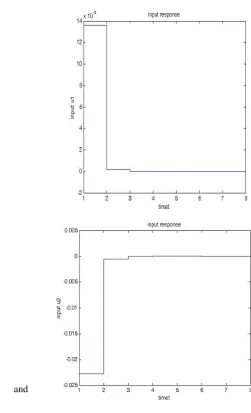
Example 1: Consider a discrete-time system with a single state delay, the problem is to find the output feedback controller matrix
K
for assigning the eigenvalue spectrum L={−0.3, -0.1, 0, 0.1, 0.3, 0.5} to the delay system.1 0 1 2 0 1 0 1
( 1) 0 1 1 ( ) 1 2 3 ( 1) 1 0 ( )
0 0 2 0 3 4 0 2
x i x i x i u i
1 0 1 1 4 0
y( ) ( ) ( 1)
0 2 3 1 0 5
i x i x i
Step 1: Inter matrices A, B, C and eigenvalues and Calculate
A
,B
andC
.1 0 1 2 0 1
0 1 1 1 2 3
0 0 2 0 3 4
1 0 0 0 0 0
0 1 0 0 0 0
0 0 1 0 0 0
A
0 1
1 0 0 2 0 0 0 0
0 0
B
1 0 1 1 4 0
0 2 3 1 0 5
C
Step 2: Obtain
X
l andX
rthat are null space ofB
ntand C respectively, then calculate
Y
l
A
tU
1,Y
r
A
X
r0.8944 0 0 0
0 0 0 0
0.4472 0 0 0
0 1 0 0
0 0 1 0
0 0 0 1
l
X
0.2517 0.2353 0.9087 0.0408 0.4414 0.1177 0.1769 0.8094 0.6369 0.1469 0.1551 0.5405 0.1517 0.9095 0.2398 0.1530
0.1842 0.2495 0.1285 0.1632 0.5284 0.1408 0.2118 0.0311
r
X
0.8944 1 0 0
0 0 1 0
0 0 0 1
1.7889 0 0 0 1.3416 0 0 0 0.8944 0 0 0
l
Y
1.2171
2.0603
0.7960
0.3065
0.0269 0.0412
0.1934
0.5357
2.8347
0.4789
0.15426
0.7161
0.2517 0.2353
0.9087
0.0408
0.4414 0.1177
0.1769
0.8094
0.6369
0.1469
0.1551
0.5405
r
Y
Step 3: Obtain
Z
[
z
1z
2
z
n]
and]
[
w
1w
2w
nW
. [12]0.0448 0 0 0 4.3395 5.1400
2.8456 0 0 0 2.5907 6.1160
Z
0.3667 0 0 0 0.1556 0.1188 0.4071 0 0 0 0.2186 0.0644
W
Step 4: Calculate matrices T,
then obtain K.
0
0
0
1
0
0
0
0
0
0
1
0
0
0
0
0
0
1
5827
.
1
3542
.
2
1505
.
3
4220
.
1
9995
.
2
1404
.
5
9571
.
0
4518
.
1
9264
.
1
1228
.
0
6482
.
0
3347
.
0
2087
.
0
3229
.
0
4248
.
0
7110
.
0
4998
.
1
5702
.
1
0.8601 0.4007
0.1173 0.0842
K
Fig. 2. The state vector Elements x(i) converge to zero.
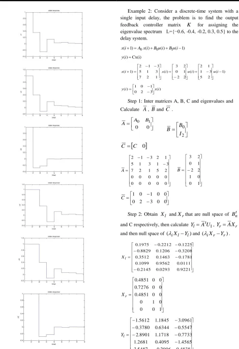
Example 2: Consider a discrete-time system with a single input delay, the problem is to find the output feedback controller matrix
K
for assigning the eigenvalue spectrum L={−0.6, -0.4, -0.2, 0.3, 0.5} to the delay system. ) 1 ( ) ( ) ( ) 1(i A0xi B0ui B1ui x
( ) Cx(i)
y i
) 1 ( 2 5 3 1 1 2 ) ( 2 2 1 0 2 3 ) ( 1 2 7 3 1 5 3 1 2 ) 1 (
xi ui ui
i x ) ( 3 2 0 1 0 1 )
(i xi
y
Step 1: Inter matrices A, B, C and eigenvalues and Calculate
A
,B
andC
. 0 0 1 0 B A A
2 0I
B
B
C
0
C
0 0 0 0 0 0 0 0 0 0 2 5 1 2 7 3 1 3 1 5 1 2 3 1 2 A 1 0 0 1 2 2 1 0 2 3 B 0 0 3 2 0 0 0 1 0 1 CStep 2: Obtain
X
l andX
rthat are null space ofB
ntand C respectively, then calculate
Y
l
A
tU
1,Y
r
A
X
rand then null space of
(
iX
l
Y
l)
and(
iX
r
Y
r)
. 0 0 0 0 0 0 2 5 3358 . 5 3 1 6082 . 4 1 2 2127 . 1 r Y
Step 3: Obtain
Z
[
z
1z
2
z
n]
and]
[
w
1w
2w
nW
. [12] 0073 . 0 0195 . 0 0036 . 0 0102 . 0 0029 . 0 0051 . 0 0260 . 0 0087 . 0 0019 . 0 0012 . 0 Z 6316 . 95 8806 . 20 5516 . 85 9751 . 62 8739 . 13 0943 . 64 4249 . 59 3578 . 29 9008 . 75 5422 . 23 W
Step 4: Calculate matrices T,
then obtain K. 0043 . 0 0059 . 0 0004 . 0 0075 . 0 0022 . 0 0029 . 0 0032 . 0 0025 . 0 0029 . 0 0013 . 0 0018 . 0 0230 . 0 0086 . 0 0023 . 0 0009 . 0 0069 . 0 0213 . 0 0027 . 0 0030 . 0 0008 . 0 0010 . 0 0049 . 0 0008 . 0 0053 . 0 0013 . 0 T 6063 . 0 0846 . 7 3584 . 0 4352 . 3 8680 . 0 1528 . 0 4396 . 1 4690 . 0 3664 . 0 0495 . 0 5442 . 2 3408 . 10 9537 . 4 6305 . 3 1100 . 1 6541 . 8 8958 . 4 9313 . 11 6128 . 7 0565 . 3 5415 . 34 1860 . 19 8291 . 43 7131 . 25 7791 . 10 1494 . 0 4936 . 4 1774 . 0 8878 . 4 K
6. CONCLUSIONS
In this research, we investigate a new method with framework for explicit formulas for output feedback controllers with linear equations in arbitrary eigenvalue assignment for linear multivariable controllable and observable systems; which is based on the matrix inverse eigenvalue problem. There are many approaches for this problem. For example, [3,11,12] state that output feedback matrix can obtain from state feedback matrix under certain conditions. This method requires solving non-linear equations therefore is very costly in gain matrices. The method proposed in this paper does not require prior knowledge of the open-loop eigenvalues and the controller does not impose any restrictions on the position of the desired eigenvalues or their nature and multiplicity. so we can use it for discrete and continues linear systems. The error of method will be zero when
B
andC
are invertible.REFERENCES
[1] H. Ahsani Tehran, “Localization of Eigenvalues in Small Specified Regions of Complex Plane by State Feedback Matrix,” J. Sci. Islam. Repub. Iran, vol 25(2), pp. 157 – 164.
[2] M.T. Chu, “Inverse eigenvalue problems,” SIAM, vol 40, pp. 1-39, 1998.
[3] Y. Dong and J. Wei, “Output feedback stabilization of nonlinear discrete-time systems with time-delay,” Advances in Difference Equations, vol 73, pp. 1-11, 2012.
[4] R. Dorf and R.H. Bishop, Modern control system, 11th Edition, Prentice Hall 2007.
[5] G.H. Golub and C.F. Van Loan, Matrix Computations, 4th Edition, The Johns Hopkins University Press, Baltimore 2013.
[6] S.M. Karbassi and D.J. Bell “Parametric time-optimal control of linear discrete-time systems by state feedback-Part 1: Regular Kronecker invariants,” International Journal of Control, vol. 57, pp. 817-830, 1993.
[7] S.M. Karbassi and F. Saadatjou, “A parametric approach for eigenvalue assignment by static output feedback,” Journal of the Franklin Institute, vol. 346, pp. 289-300, 2009.
[8] S.M. Karbassi and H.A. Tehrani, “Parameterizations of the state feedback controllers for linear multivariable systems,” Computers and Mathematics with Applications, vol. 44, pp. 1057-1065, 2002. [9] R.W. Koepcke, “On the control of linear systems
with pure time-delay,” Trans. ASME Journal of Basic Engineering, vol. 87, pp. 74-80, 1965.
[10] F. Kurzweil, “The control of multivariable processes in the presence of the pure transport delays,” IEEE Trans. Automatic Control, vol. 8, pp. 27- 35, 1963. [11] N. Li, “An iterative method for pole assignment,”
Linear Algebra and Its applications, vol. 23, pp. 77-102, 2001.
[12] N. Li, “An inverse eigenvalue problem and feedback control,” proceedings of the 4th Biennial engineering mathematics and applications conference, vol. 124, pp. 183-186, 2000.
[13] X. Li and H. Gao, “A new model transformation of discrete-time systems with time-varying delay and its application to stability analysis,” IEEE Transactions on Automatic Control, vol. 56, no. 9, pp. 2172–2178, 2011.
[14] S.M. Modarres and S.M. Karbassi, “Time-optimal control of discrete time linear systems with state and input time-delays,” International Journal of Innovative Computing, Information and Control, vol. 5, no. 9, pp. 2619-2625, 2009.