External Support Vector Machine Clustering

University of New Orleans University of New Orleans

ScholarWorks@UNO

ScholarWorks@UNO

University of New Orleans Theses and

Dissertations Dissertations and Theses

8-9-2006

External Support Vector Machine Clustering

External Support Vector Machine Clustering

University of New Orleans

Follow this and additional works at: https://scholarworks.uno.edu/td

Recommended Citation Recommended Citation

McChesney, Charlie, "External Support Vector Machine Clustering" (2006). University of New Orleans Theses and Dissertations. 409.

https://scholarworks.uno.edu/td/409

This Thesis is protected by copyright and/or related rights. It has been brought to you by ScholarWorks@UNO with permission from the rights-holder(s). You are free to use this Thesis in any way that is permitted by the copyright and related rights legislation that applies to your use. For other uses you need to obtain permission from the rights-holder(s) directly, unless additional rights are indicated by a Creative Commons license in the record and/or on the work itself.

EXTERNAL SUPPORT VECTOR MACHINE CLUSTERING

A Thesis

Submitted to the Graduate Faculty of the University of New Orleans in partial fulfillment of the requirements for the degree of

Master of Science in

Computer Science

by

Charles B. McChesney III

B.S. Computer Science University of New Orleans, 2004

Table of Contents

Abstract... 1

I. Introduction ... 2

II. Background ... 2

III. Methods... 12

IV. Results ... 19

V. Discussion ... 28

VI. Conclusion ... 35

VII. References ... 37

Appendix A………39

Abstract. The external-Support Vector Machine (SVM) clustering algorithm clusters

data vectors with noa priori knowledge of each vector’s class. The algorithm works by

first running a binary SVM against a data set, with each vector in the set randomly

labeled, until the SVM converges. It then relabels data points that are mislabeled and a

large distance from the SVM hyperplane. The SVM is then iteratively rerun followed by

more label swapping until no more progress can be made. After this process, a high

percentage of the previously unknown class labels of the data set will be known. With

sub-cluster identification upon iterating the overall algorithm on the positive and negative

clusters identified (until the clusters are no longer separable into sub-clusters), this

method provides a way to cluster data sets without prior knowledge of the data’s

I. Introduction

An ideal clustering algorithm can perfectly determine the clusters in a data set with no

supervision regardless of the shape, noise-level, and similarity of the clusters in the set.

At present, none of the popular clustering algorithms are ideal. Instead, some methods

perform strongly on similar clusters, but weakly on arbitrarily shaped clusters. Other

methods perform very well on non-overlapping clusters, but become unreliable when the

data contains noise. And the best performing methods require supervision, often

requiring the tuning of multiple dependant parameters by an experienced user.

In this paper, an External SVM clustering algorithm is presented. This algorithm

provides an alternative method to the current clustering algorithms, which (when

automated) requires no supervision, easily distinguishes arbitrarily shaped clusters, is

resistant to noise, and separates clusters that strongly overlap. The performance of this

algorithm is examined on real DNA hairpin data and two-dimensional artificial data, and

is compared to the results of the other popular clustering methods.

II. Background

Support Vector Machines

SVM’s are learning machines, which provide good generalization performance for

classification tasks. They have been used for pattern recognition in many tasks including:

isolated handwritten digit recognition, object recognition, speaker identification, face

detection in images, and text categorization. This section will provide a brief

introduction to the inner workings of SVM’s. For a more detailed explanation of SVM’s,

see the papers of Scholkopf, Burges, and Vapnik of Bell Laboratories [12].

The goal of SVM’s is, for a given learning task, with a given finite amount of training

data, to achieve the best generalization performance by striking the right balance between

the training set without error [12]. In comparison with neural net learning machines,

which overfit easily based on local anomalies, SVM’s use structural risk minimization to

minimize the risk of overtraining and provide unique global solutions.

To begin, let us assume there is a learning problem withl observations. Each observation

consists of a data vector,xi, and an associated label,yi. The task of the SVM is to learn

the mapping of eachxi to eachyi. The functionf(x,α), whereα is an adjustable

parameter, will determine this mapping. This function is deterministic, in that for a given

x, and a choice ofα, it will always give the same output. A particular choice ofα

generates a trained machine. The expected test error of a trained machine is therefore:

(1)

The goal of structural risk minimization is to reduce the expected risk of error. This is

obtained through the following equation:

(2)

HereRemp(α) is the empirical risk. The empirical risk is defined to be the measured mean

error rate on the training set. The letterh is a non-negative integer called the Vapnik

Chervonenkis (VC) dimension, and is a measure of the amount the machine can learn

without error. ηis a chosen loss parameter between 0 and 1. The second term on the

right hand side is the “VC confidence”. The above risk minimization equation says that

given several learning machines, defined byf(x,α), we can calculate each machine’s risk.

This is the essential idea of structural risk minimization. Given a fixed family of learning

Now, lets discuss the VC dimension. Givenl points, and for each labeling, if a member

of the set{f(x)} can be found which correctly assigns those labels, then that set of points

is “shattered” by that set of functions. The VC dimension for the set of functions{f(x)} is

defined as the maximum number of training points that can be shattered by{f(x)}.

SVM’s define a hyperplane which separate the data point’s labels. On one side of the

hyperplane labels will be positive (denoted by 1), and the other side negative (denoted by

–1). We will now introduce a theorem.

THEOREM- Consider some set of m points inRn. Choose any one of the points as

origin. Then m points can be shattered by oriented hyperplanes if and only if the position

vecors of the remaining points are linearly independent [12].

Corollary: The VC dimension of the set of oriented hyperplanes inRn isn+1, since we

can only choosen+1 points, and then choose one of the points as origin, such that the

position vectors of the remainingn points are linearly independent, but can never choose

n+2such points (since non+1 vectors inRn can be linearly independent) [12].

(Note: A proof of this theorem and corollary can be found in [13].)

The VC confidence is a monotonic increasing function ofh. This will be true for any

value ofl. Thus, given some selection of learning machines, one wants to choose the

learning machine whose associated set of functions has a minimal VC dimension. This

will lead to an upper bound on the actual error. In general, one wants to reduce the VC

confidence. (Note: This only acts as a guide. Infinite VC dimension (capacity) does not

guarantee poor performance).

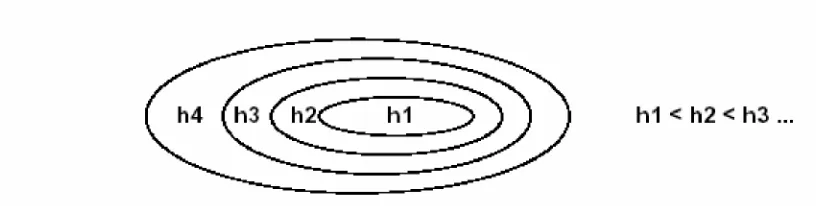
Structural risk minimization (SRM) finds the subset of the chosen class of functions (for

a training problem), so that the risk for that subset is minimized. This is done by

introducing a “structure” which divides the entire class of functions into a set of method

subsets. Structural risk minimization then consists of finding that subset of functions,

machines, one for each subset, where for a given subset the goal of training is to

minimize the empirical risk. Then take that trained machine in the series whose sum of

empirical risk and VC confidence is minimal.

Figure 1. Nested subsets of functions, ordered by VC dimension.

Now we will illustrate how the hyperplane separates the different classes of data vectors.

The following constraint determines the class for each vector.

(3)

This constraint is replaced by constraints on Lagrange multipliers, so that the training

data appears in the form of dot products between vectors. This property allows

generalization to the non-linear case. Below are the primal and dual Lagrangian.

(4)

(5)

The½||W||2term in (4) represents the structural risk minimization term corresponding to

the hyperplane having the largest possible margin, and thus limiting the risk of error. LP

solution is found by minimizingLP or maximizingLD. Support vector training therefore

amounts to minimizingLP or maximizingLD with respect to certain constraints. There is

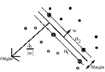
a Lagrange multiplier for every training point. In the solution, those points for which αi > 0 are called support vectors, and lie on one of the hyperplanesH1 orH2. All the

other training points haveαi = 0and lie onH1 orH2, or lie on the positive or negative

side ofH1 orH2 [12].

Figure 2. Linear separating hyperplane for the separating case. The support vectors are

circled.

Now we will discuss the Karush-Kuhn-Tucker (KKT) conditions. The KKT conditions

are satisfied at the solution of any constrained optimization problem, with any kind of

constraints, provided the intersection of the set of feasible directions with the set of

descent directions coincides with the intersection of the set of feasible directions for

linearized constraints with the set of descent directions. The KKT conditions are

analogous to the equations of motion that are obtained from the Lagrangian in classical

mechanics. Solving the SVM problem is equivalent to finding the solutions of the KKT

conditions. Below are KKT conditions corresponding to the Lagrangian shown in

equation(4) (see [12] for further details).

(7)

(8)

(9)

from∂ /∂αi LP= 0, whenα i is restricted to be >=0.

(10)

this results from combining (8) and (9) under the conditions where their negative

contribution to the Lagrangian must be reduced to zero for the Lagrangian LP to

be maximized.

Now we will explain how the kernel is used. We need to put into the form of dot

products. Mapping to some other (possibly infinite) dimensional Euclidean space would

cause the training algorithm to only depend on the data through dot products in the

Euclidean space,H. Now, if there were a kernel functionK, such that K(xi,xj)=F(xi)

F(xj), onlyK would be needed in the training algorithm (F() corresponds to mapping xi

andxj intoH). The kernel allows for the mapping of the training data into kernel space.

The Gaussian kernel is:

(11)

For this kernel function,H is infinite dimensional, and allows production of a support

vector machine which lives in infinite dimensional space, and it also allows the SVM to

train roughly in the same time as the unmapped data. Since most SVM’s function best

VC-confidence is marginalized in actual application, beyond its contribution to the

original incorporation of SVM concepts.

Clustering

Clustering is an unsupervised learning problem, whose goal is finding a structure in a

collection of unlabeled data. A cluster is a collection of objects, which are similar to the

other objects in that collection and dissimilar to the objects belonging to the other clusters

[3]. Clustering can be used in almost any field. Some applications of clustering include

search engine document classification, finding groups of customers with similar buying

patterns, image clustering for computer forensics, DNA hairpin classification, and

knowledge discovery in a general setting, where feature or concept primitives themselves

need to be identified.

Distance measure is an important component of clustering algorithms. If the data vectors

are all in the same physical units, then a Euclidean distance metric can be used. In some

cases where the units do not match or are some nominal unit, domain knowledge must be

used to formulate a suitable distance formula. Still, in cases where Euclidean distance

can be used, the choice of the mathematical formula used for the clustering distance

measure will affect the clustering groupings.

The two basic types of clustering are hierarchical and partitional [6]. Hierarchical

clustering finds new clusters using previously established clusters [8]. Partitional

clustering can be further subdivided into exclusive, overlapping, and model-based

clustering [2]. Exclusive clustering groups data points in an exclusive way, so that if a

certain point belongs to one cluster, then it cannot be included in another cluster.

Overlapping clustering uses fuzzy sets to cluster data, so that each point may belong to

more than one cluster with different degrees of membership. Each point will be related to

each cluster by its membership value. Finally, model-based clustering uses models for

clusters and attempts to optimize the fit between the model and the data. Next, the four

Hierarchical Clustering

“Bottom-up” hierachical clustering is based on the union between the two nearest cluster.

Initially, all data vectors will represent their own cluster, and iteratively clusters will be

joined by union to the nearest cluster, until the final desired cluster representations are

reached. Hierarchical clustering can also be approached from the “top-down”. In this

approach, all data vectors are initially members of the same cluster. This cluster will be

split into two clusters by optimal bisection, and then iteratively all new clusters will be

split until the desired number of clusters is reached. The External-Relabel SVM

clustering algorithm uses a variation of “top-down” hierarchal clustering for multiple

cluster identification.

K-means Clustering

K-means clustering is an example of exclusive clustering. The procedure classifies a

given data set through a certain number of clusters (“K” clusters are chosen a priori).

The following steps represent the algorithm:

1. Randomly place K points into the data space. These points represent the initial

cluster centroids.

2. Assign each data vector to the cluster that has the “closest” centroid.

3. When all the data vectors have been assigned, recalculate the position of the K

centroids. This calculation is done making each centroid the minimizer of the

distance-based objective function of its associated cluster.

4. Repeat steps 2 and 3 until the centroids no longer move. This produces a

separation of the data objects into clusters for which the chosen Euclidean

Figure 3. Illustrates the k-means algorithm steps, from initial centroid placement to final

cluster definitions.

In general, the algorithm aims to minimize someobjective function. The objective

function used in k-means algorithms is the squared distance function, which consists of a

double summation on||xij-cj||2. Here||xij-cj||2 is the chosen distance measure between a

data vector xij and the cluster centroid cj. This objective function is an indicator of the

variance of the ndata vectors from their respective cluster centroids.

There are several problems with the K-means algorithm. First of all, since the number of

clusters must be known a priori, the algorithm by itself cannot solve problems where the

number of clusters is unknown. Next, the algorithm does not always find the most

optimal clusters because the objective function used does not always use the best distance

metric for the problem. Finally, the location of the initial random cluster centroids can

heavily influence the resulting clusters, creating the probability that the final clusters will

be trapped in a local minima of the objective function.

Kernel K-means Clustering

Kernel K-means is a K-means clustering algorithm, in which a kernel is used to map the

data into a higher dimensional space. Kernel functions perform a non-linear

transformation of the data by mapping it into a space where the separability of the data is

increased [5]. The distance measure,||xij-cj||^2, in the objective function of the K-means

algorithm is therefore transformed by some kernel function [11]. In this paper, the

the data vectors are run through an SVM, which improves the clustering accuracy by

dropping data with weak clustering scores.

Robust Kernel Fuzzy Clustering

Robust Kernel Fuzzy clustering is an example of overlapping clustering, which allows

each data vector to belong to more than one cluster. It is an alternative to the popular

Fuzzy C-Means clustering, which is an overlapping clustering method developed by

Dunn and extended by Bezdek [6]. The Robust Kernel Fuzzy clustering method adopts

the fuzzy partition matrix in its objective function (from Fuzzy C-Means clustering),

. The fuzzy partition matrix, xij, allows data points to have membership values

in each of the clusters [9]. In contrast to the Fuzzy C-Means method, the Robust Kernel

Fuzzy clustering uses a kernel, which is incorporated to allow the method to recognize

arbitrarily shaped clusters [10]. The method gains robustness through the modification of

the Euclidean distance formula in its objective function from to [9].

This clustering algorithm is similar to the K-means algorithm, in that it aims to minimize

its objective function when determining a data vector’s cluster membership. It is

different, because it includes a fuzzy partition matrix, which scores each data vector’s

membership value with every cluster in the problem. The Robust Kernel Fuzzy clustering

algorithm implemented for this paper is described in the Methods section.

Mixture of Gaussians

Mixture of Gaussians is an example of model-based clustering. In this approach, clusters

are considered Gaussian distributions centered on their centroids. The Expectation

Maximization (EM) [4] algorithm is used to find the Gaussian distributions, which model

the data. In the clustering process used in this paper, Gaussian distributions model

clusters in both the preprocessing (Kernel K-means) and External-Relabel SVM

DNA Hairpin Data

The DNA hairpin data clustered in this paper is created by running raw data through a

tFSA/HMM, which creates a data set that contains 151 feature vectors for each element.

A description of the raw data can be found in Appendix E of [15].

III. Methods

Single Class SVM Clustering

The Single Class SVM clustering method was developed by Vapnik [14]. It is able to

perform multi-cluster separation in a single SVM run, by enclosing clusters in

hyperspheres. A hypersphere is similar to a hyperplane in that it is a boundary, in

possibly infinite dimensional kernel space, which separates data vectors of different

classifications. It is different than a hyperplane because, instead of only separating the

data vectors with different classifications, it surrounds the data allowing for more than 2

classes to be defined. For clusters where there is not total separation between the

respective members, a drop zone must be added to split the clusters. The following

paragraphs describing this clustering method are from our recent publication on SVM

classification and clustering in the MCBIOS proceedings in BMC Bioinformatics [1].

Let {xi} be a data set of ‘N’ points in Rd. Using a non-linear transformation , we

transform ‘x’ to some high-dimensional space called Kernel space and look for the

smallest enclosing sphere of radius ‘R’. Hence we have: || (xj) - a ||2 R2 for all j =

1,…,N; where ‘a’ is the center of the sphere. Soft constraints are incorporated by adding

slack variables ‘ j’:

|| (xj) - a ||2 R2 + j for all j = 1,…,N

Subject to: j 0 (12)

We introduce the Lagrangian as:

Subject to: j 0, j 0, (13)

where C is the cost for outliers and hence C j j is a penalty term. Setting to zero the

derivative of ‘L’ w.r.t. R, a and we have: j j = 1; a = j j (xj); and j = C - j.

Substituting the above equations into the Lagrangian, we have the dual formalism as:

W = 1 - i,j i jKij where 0 i C; Kij = exp(-||xi – xj||2/2 2)

Subject to: i i = 1 (14)

By KKT conditions we have: j j = 0 and j(R2 + j - || (xj) - a ||2) = 0.

In the kernel space of a data point ‘xj’ if j > 0, then j = C and hence it lies outside of the

sphere i.e. R2 < || (xj) - a ||2. This point becomes a bounded support vector or BSV.

Similarly if j = 0, and 0 < j < C, then it lies on the surface of the sphere i.e. R2 = || (xj)

-a ||2. This point becomes a support vector or SV. If j = 0, and j = 0, then R2 > || (xj) - a

||2 and hence this point is enclosed within the sphere.

Kernel K-Means Clustering

The data is first mapped into kernel space. The following absdiff kernel is used:

exp(

−

1/2(

∑

|x

-x

|) / 2

σ

)

(Note: For more information on the absdiff kernel, check out Appendix A.)

Next the K-Means algorithm is performed on the data in kernel space.

The K-Means implementation used in this paper is very similar to the K-Means algorithm

described in the background section, with a couple of exceptions. First of all, our

implementation uses the constraint that every problem always has at most two clusters

(one cluster can also be obtained when the data cannot be separated into two clusters).

Further cluster identification is obtained through iteratively clustering the results of prior

defined in the first step of the algorithm. Instead of randomly picking a cluster centroid

in the data space explicitly, the initial centroids are defined by the initial random labeling

of the data vectors. Each vector is randomly labeled with a 50% chance of being positive

and a 50% chance of being negative, and the two centroids are defined as the barycenter

of their respective data vectors. Hence the initial cluster centroids are implicitly random,

since their locations are determined by the random locations of their members.

Robust Kernel Fuzzy Clustering

The Robust Kernel Fuzzy clustering method aims to perform better than the Kernel

K-Means algorithm, through providing more resistance to noisy data through changing the

Euclidean distance formula used in the objective function from to

[9]. Data can be dropped by setting a minimum membership score requirement. Then,

using the fuzzy partition matrix, the data points that do not meet the minimum score

requirement for any clusters are dropped. This paper implements the algorithm described

in [9] exactly. For a more thorough description of the algorithm, see [9].

External-Drop SVM Clustering

The External-Drop SVM clustering method improves the accuracy on a data set that has

already been split into two clusters. In this paper, we use this method after the Kernel

K-Means algorithm has separated a set of data into clusters. The External-Drop SVM then

acts as a filter, dropping all data that isn’t strongly identified with either cluster, and thus

improving the cluster identifications. The SVM can then be iteratively rerun, defining a

more accurate hyperplane for clustering the current data, and for cluster classification of

new similar data. The, weaker linear kernel,xi•xj, is used in the SVM, because it does not

overfit the data in this circumstance. The algorithm is as follows:

1. After the data is labeled by the Kernel K-Means clustering step, it is run through a

2. All the data vectors, which are identified as support vectors (bounded and

unbounded) by the SVM, are dropped.

3. The SVM is then rerun on the updated data set (updated data set = original data

set – dropped data).

4. Repeat steps 2 and 3 until an acceptable amount of data has been dropped.

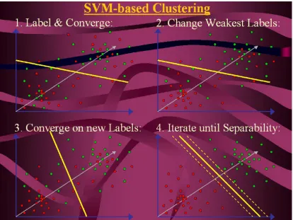
External-Relabel SVM Clustering

The External-Relabel SVM clustering algorithm clusters data by relabeling the data

vectors, which are strongly mislabeled. Strongly mislabeled data are vectors, which are a

large distance away from the hyperplane, relative to the other mislabeled data. The

following is a simple step-by-step description of the basic algorithm used for

External-Relabel SVM-clustering:

1. Start with a set of data vectors.

2. Randomly label each vector in the set as positive or negative.

3. Run the SVM on the randomly labeled data set until convergence is obtained

(random relabeling is needed if prior random label scheme does not allow for

convergence).

4. After initial convergence is obtained for the randomly labeled data set, relabel

the misclassified data vectors, which have confidence factor values greater than

some threshold (vectors with larger confidence factor values are farther away

from the hyperplane).

5. Rerun the SVM on the newly relabeled data set.

6. Continue relabeling and rerunning SVM until no vectors in the data set are

Figure 4. Illustrates the External-Relabel SVM clustering process.

Relabeling Methods

The relabeling function is implemented in several different overriding ways. For the

results of this paper all misclassified vectors were flipped according to the following

pseudo-code:

For positive vectors that are mislabeled,

if(abs(Ci)>abs(sum(Ci...Cj)/j)) {

flip label;

} (16)

Where Ci is the confidence factor value for the mislabeled vector,

For negative vectors that are mislabeled,

if(Ci>(sum(Ci-Cj)/j)) {

flip label;

} (17)

Where Ci is the confidence factor value for the mislabled vector,

and there are j mislabled negative vectors.

It is important to note that this scheme considers the positive and negative mislabeled

vectors as disjoint sets. This is done because the hyperplane created may be skewed to

either the positive or negative side (confidence values of the positive misclassified

vectors may be much higher than the confidence values of the negative misclassified

vectors and vice versa). By separating the positives from the negatives, the scheme

avoids improperly exploiting this imbalance.

Next, the simplest scheme used is the tui(textual user interface) scheme. In this scheme,

statistics describing the misclassified vectors are output to the user. The statistics used

are the value of the farthest outlier(farthest away from hyperplane), the value of the

closest outlier(closest to hyperplane), the average value, the standard deviation, and the

number of vectors. This information is then used to make a decision about which vectors

should be flipped. The user enters a threshold value at which all misclassified vectors

with greater confidence factor values are relabeled. The flipping conditions are:

Separately for the positive and negative vector sets that are mislabeled,

for(Ci...Cj) {

if(abs(Ci)>abs(Cv)) {

flip label;

}

} (18)

Where Ci is the confidence factor value for the mislabeled vector,

Another promising scheme relabels misclassified vectors in the same way as above

except it flips a percentage of the worstly misclassified vectors. As before, the positive

and negative vectors must be separated. The pseudo-code is:

For vectors that are mislabeled,

@sorted = descending_sort(abs(Ci...Cj));

n=total_vectors*percent_to_flip;

for(@sorted) {

flip label of sorted[0]...sorted[n-1];

} (19)

Where Ci is the confidence factor value for the mislabeled vector,

there are j mislabeled vectors, and n is the total misclassified

positive vectors multiplied by the percentage of vectors to flip.

Process must be done separately for the positive and negative misclassified

vector sets.

The advantage to this method is greater control over the number of vectors relabeled on

each iteration. The percentage of misclassified vectors provides the user with a moer

controllable threshold parameter.

SVM Parameters

The SVM Background section explains SVM parameterization in greater detail. This

section will talk about the different svm parameters that were tuned for clustering

purposes.

Implementations

The W-H SMO and Keerthi’s SVM implementation are both used. The W-H SMO,

from Platt based implementations in that it only chooses one alpha in each optimization

step, while the other alpha is automatically specified. All other SMO implementations

have to choose two alphas for optimization.

Kernels

Abs-diff, Gaussian, and Linear kernels are all used (see Appendix A). The Gaussian

kernel is used for the External-SVM relabeling method. The Abs-Diff kernel is used in

the Kernel K-Means implementation. The Linear kernel is used for dropping data in the

External-SVM drop method.

Sigma(squared)

The choice of the

σ

achieving accurate clustering results. The

σ

properly fit the data. This is illustrated in the results section.

Allowed KKT Violators

For the External-Relabel SVM clustering method, KKT violators must often be allowed

to obtain initial convergence, because the random labeling scheme is likely to cause

violators. However increasing the allowed KKT violators can reduce the accuracy of the

hyperplane. Also, for this clustering method, if the SVM converges and creates a

hyperplane that is inaccurate enough, the relabeling may cause the svm to fail to

converge on the next iteration. If this happens, convergence may never be obtained

again, so the program must be halted and restarted. So tuning may be needed on the

number of violators to find a number that is large enough to allow convergence, but small

enough to not strongly affect accuracy.

8GC/9GC DNA Hairpin Data

0.4 0.5 0.6 0.7 0.8 0.9 1

1

Clustering Methods

SVM Relabel (Drop)=16.1% drop K K-Means (SVM Drop)=22.8%

drop

Per

centa

ge

of

Corr

ectly

Clustered

Data

Vectors

SVM Relabel

SVM Relabel (Drop) K K-Means

K K-Means (SVM Drop) Robust Fuzzy

Robust Fuzzy (Drop) Single Class SVM

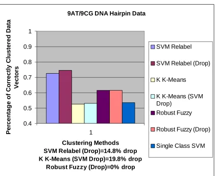
9AT/9CG DNA Hairpin Data 0.4 0.5 0.6 0.7 0.8 0.9 1 1

Clustering Methods

SVM Relabel (Drop)=14.8% drop K K-Means (SVM Drop)=19.8% drop

Robust Fuzzy (Drop)=0% drop

Per centag e of Corr ectly Clustered Data Vectors SVM Relabel

SVM Relabel (Drop)

K K-Means

K K-Means (SVM Drop)

Robust Fuzzy

Robust Fuzzy (Drop)

Single Class SVM

Figure 6. Accuracy comparison of each method s run on the 9AT/9CG DNA

hairpin data.

Note: This is a much more challenging cluster separation problem than the data

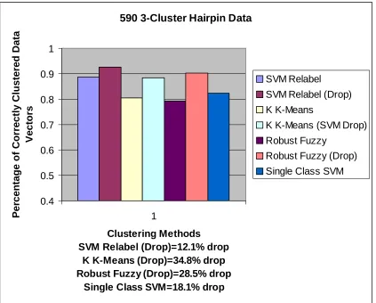
590 3-Cluster Hairpin Data

0.4 0.5 0.6 0.7 0.8 0.9 1

1

Clustering Methods SVM Relabel (Drop)=12.1% drop

K K-Means (Drop)=34.8% drop Robust Fuzzy (Drop)=28.5% drop

Single Class SVM=18.1% drop

Per

centage

of

Correctly Clustered

Data

Vectors

SVM Relabel

SVM Relabel (Drop) K K-Means

K K-Means (SVM Drop) Robust Fuzzy

Robust Fuzzy (Drop) Single Class SVM

Figure 7. Accuracy comparison of each method s run on the first iteration for the

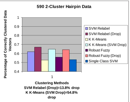
590 2-Cluster Hairpin Data

0.4 0.5 0.6 0.7 0.8 0.9 1

1

Clustering Methods

SVM Relabel (Drop)=13.8% drop K K-Means (SVM Drop)=54.8%

drop

Per

centag

e

of

Corr

ectly

Clustered

Data

Vectors

SVM Relabel

SVM Relabel (Drop) K K-Means

K K-Means (SVM Drop) Robust Fuzzy

Robust Fuzzy (Drop) Single Class SVM

Figure 8. Accuracy comparison of each method s run on the second iteration for the

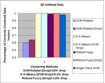
2D Artificial Data 0.4 0.5 0.6 0.7 0.8 0.9 1 1 Clustering Methods SVM Relabel (Drop)=15% drop K K-Means (SVM Drop)=0.1% drop

Robust Fuzzy (Drop)=1.6% drop

Per centag e of Corr ectly Clustered Data Vectors SVM Relabel

SVM Relabel (Drop)

K K-Means

K K-Means (SVM Drop)

Robust Fuzzy

Robust Fuzzy (Drop)

Single Class SVM

Figure 9. Accuracy comparison of each method s run on the 2D artificial data.

Note: This two-dimensional data contains two clusters with equal total width,

completely separated by 10 times this width in the first dimension. This is a trivial

problem for other clustering methods, but can cause the SVM Relabel method to

enter deadlock if the initial chosen random labeling scheme is poor. This data result

highlights a key difficulty with the current SVM Relabel method. Currently, several

approaches are being researched, most notably using the Kernel K-Means as a

preprocessing step, which creates a non-random initial labeling scheme, preventing

the deadlock scenario Such preprocessing should reduce or remove the possibility

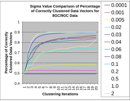
Sigma Value Comparison of Percentage of Correctly Clustered Data Vectors for

8GC/9GC Data 0.4 0.5 0.6 0.7 0.8 0.9 1

1 2 3 4 5 6 7 8 9

10 11 12 13 14 15 16 17 18 19 20

Clustering Iterations Per centa ge of Corr ectly Clustered Data Vectors

0.0001

0.001

0.005

0.02

0.03

0.04

0.06

0.08

0.1

0.2

0.5

1.0

2

Figure 10. Accuracy comparison for External-Relabel SVM clustering runs on the

8GC/9GC DNA hairpin data using differentσ2 values.

Note: Theσ2value of 0.2 performs optimally, with a stable fall-off in performance

asσ2 is moved off of this value. Theσ2 choices are pushed to the extremes 0.0001

and 2.0 to show how poor choices eventually lead to complete failure (a percentage

correct of 50% is the equivalent of random guessing in such sets where the clusters

Runtime Comparison (8GC/9GC Data)

0 100 200 300 400 500 600 700 800 900 1000

1

Clustering Methods

Time (

s)

SVM Relabel

SVM Relabel (Drop)

Kernel K-Means

Kernel K-Means (SVM Drop)

Robust Fuzzy

Roubst Fuzzy (Drop)

Single Class SVM

Figure 11. Runtime comparison of all clustering methods on the 8GC/9GC DNA

Average Runtimes - Keerthi vs.

W-H SMO

0

200

400

600

800

1000

1

SVM Implementations

Aver

age

Runti

me in s

Keerthi

W-H SMO

Figure 12. External-Relabel SVM clustering runtime comparison between the

V. Discussion

External-Relabel SVM Clustering

The External-Relabel SVM Clustering method performed very well on the real DNA

hairpin data, but poorly on the artificial two-dimensional data. The poor performance on

the artificial 2D data may be because there isn’t enough information in the two

dimensions for the SVM to obtain enough statistical evidence to accurately define the

clusters. This can cause the External-Relabel Clustering method to enter deadlock if the

initial chosen random labeling scheme is poor

The results from figure 5 show that this method successfully clustered the 8GC/9GC

DNA hairpin data with almost 95% accuracy when including a drop zone. This is an

excellent result on real data, because the 8GC and 9GC data are dissimilar with little

overlap, and so should be split into two clearly separate clusters. Only the Robust Fuzzy

Clustering method had accuracy as good as the External-Relabel SVM clustering on this

data set.

Next, the results of the binary clustering runs on the 9CG/9AT DNA hairpin data are

shown in figure 6. As opposed to the 8GC/9GC data set, the 9CG and 9AT data vectors

are very similar, with a great deal of overlap. The graphs illustrating the results show that

the data vectors only separate into clusters at around 72% accuracy. In this case, it was

not surprising that the data vectors did not separate as accurately into well-defined

clusters. This is because, even in the kernel space, the similarity between the data causes

some of the outlier vectors of each class to overlap. The low confidence data may be

“common mode” noise of the two data classes, which the SVM kernel fails to

disambiguate because they fall too close to the hyperplane (these points can be removed

by dropping all the points within a large enough range from the hyperplane), or just data

representing weak properties of their classification. In SVM classification, such low

confidence data have been shown to diminish the accuracy of the hyperplane separating

3% improvement in accuracy. It should be noted that this clustering method’s

performance was clearly superior to any other method on this data set. This suggests that

the External-Relabel SVM clustering may be able to cluster complex, overlapping data

sets better than the other methods.

The initial sub-clustering results for the binary clustering runs on the 592/595/597 DNA

hairpin data are demonstrated in figure 7. Here, the 592 and 595 data sets form a separate

cluster from the 597 data set with almost 90% accuracy (an accuracy of 93% is obtained

when dropping 12% of the data). The SVM Relabel accuracy for this case is higher than

all the other methods. This is a promising first step, since the 592 and 595 data sets are

similar, while the 597 data set is not. Next, the sub-clustering algorithm will iteratively

perform the same External-Relabel SVM clustering algorithm on the results of the

previous iteration (the 592/595 and the 597 clusters). The results are shown in figure 8.

When the algorithm tries to separate the 597 cluster by itself, two clusters are produced

with an accuracy of about 50%. This is an indication that no improvement could be made

from the initial random labeling, which accurately suggests that this data set contains

only one cluster (which is true). The next iteration, which attempts to separate the 592

and 595 data sets, only results in clusters that are about 67% accurate. This result is

analogous to the 9CG/9AT results, as the 592/595 data sets’ features are also very

similar. The accuracy of this outcome is higher for the SVM Relabel method than all the

other methods, which again highlights the strength of this clustering method in separating

complex and similar data sets. This process also illustrates how multi-cluster

classification is done through iterating on the binary clustering method.

The last data set tested illustrates a key weakness with the External-Relabel SVM

Clustering method when dealing with trivially separable data. The results are illustrated

in figure 9. The two-dimensional artificial data set consists of clusters that have a

variance of four units centered around a common mean. Each cluster’s barycenter, which

is the mean of all the data points in the cluster, is separated by twenty units in one

dimension. The clusters unmistakably do not overlap, with the closest points between the

visualize this data set as clearly being in two clusters, yet this method was barely able to

separate the clusters with 60% accuracy. Furthermore, all the other clustering methods

were able to separate these clusters with close to 100% accuracy. The failure of this

method in clustering such an uncomplicated data set can easily be prevented with simple

pre-processing steps. Rather than use an ad-hoc approach, it appears best to preprocess

with some a method such as Kernel K-Means as discussed in Figure 11.

Now the various parameters used in the External-Relabel SVM Clustering method will be

discussed. This method relies on the following parameters: allowed KKT violators,

choice of

σ

will be discussed below.

The allowed KKT violators did not affect the chance of convergence or control the initial

accuracy of the hyperplane as expected. Instead allowing the minimum KKT violators

(no violators) usually did not stop initial convergence, and did not guarantee that the

initial hyperplane was accurate enough for good clustering results. If using more than the

minimum KKT violators provides no benefit in all cases (as has been observed so far),

this parameter can be removed.

The value of the sigma squared parameter heavily affected the clustering results,

indicating a tuning on this parameter is necessary. Results depicting the importance of

the sigma squared are shown in figure 10. It can be seem that with the right choice of the

sigma squared tuning parameter, the data set’s clusters are identified with over 90%

accuracy, and with the wrong sigma squared the accuracy is only 50%. Note, that the

sigma squared value must be tuned so that the Gaussian kernel fits the data well.

The random labeling scheme may be the parameter that has the greatest affect on this

method, because it determines the location of the initial hyperplane, and is the hardest to

tune. Since this method decides the final clusters by iteratively improving on its

hyperplane, the final result is heavily dependant on its initial hyperplane. One general

if all labels are deemed correct, then no relabeling can be done. This situation allows for

no correction of the initial hyperplane, and gives final clustering results that are random.

When using this method, if too few vectors are considered mislabeled by the initial

hyperplane, the vectors should be randomly relabeled. The SVM can be then run again

on the data set with the new labels, hopefully creating a better initial hyperplane.

Creating an improvable initial hyperplane is the most challenging problem to the

External-Relabel SVM Clustering method. More testing to determine the characteristics

of an acceptable initial hyperplane needs to be done. This can be directly resolved in

hybrid approaches, as mentioned previously, and is an area of future research.

W-H SMO vs. Keerthi

Both the W-H SMO (an variation of Platt’s SMO) and Keerthi’s SVM implementations

were tested in the External-Relabel SVM Clustering method. Both implementations

provided similar accuracy. The Keerthi implementation always converges, partly

accounting for a slightly faster runtime. Figure 12 shows that the Keerthi

implementation runs about 50% faster than the W-H SMO implementation. The W-H

SMO may be the safer option, since it will reject random labeling schemes that don’t

converge.

Kernel K-means Clustering

The Kernel K-Means Clustering method performed extremely well on the

two-dimensional artificial data, but only moderately well on the real DNA hairpin data. This

method has difficulty differentiating some data sets with overlapping members.

This method was unable to separate either the 8GC/9GC or 9CG/9AT DNA hairpin data,

assigning only approximately 55% of the data vectors to the correct cluster [Figures 5 and

6]. These are the worst results of all the methods for these data sets. This result

highlights the inability of the K-Means method to differentiate complex clusters that have

For the initial multi-clustering iteration, the Kernel K-Means method respectably split

slightly over 80% of the data vectors into their correct clusters. With the addition of a

relatively large 35% drop, the accuracy reaches nearly 90% [Figure 7]. On the next

iteration, the two-cluster data set can only be separated with slightly over 50% accuracy.

With a very large 60% drop, the clustering accuracy reaches nearly 65% [Figure 8]. The

results from the initial iteration suggest that the Kernel K-Means method has the ability to

cluster some complex data sets, which only slightly overlap.

Next, from figure 9, the Kernel K-Means method separates two-dimensional artificial

data set into two perfect clusters with 100% accuracy. This result highlights the strength

of this method: splitting simple, clearly defined clusters that have zero overlap.

Next, the implementation decisions and parameters will be discussed. Both the absdiff

and Gaussian kernels were implemented for this Kernel K-Means Clustering method.

The absdiff kernel performed better than the Gaussian on the DNA hairpin data, using the

Gaussian kernel resulted in higher accuracy on the two-dimensional artificial data.

The SVM Drop uses a linear kernel because Gaussian and absdiff overfit, while the linear

kernel provides room for drop (k+1 VC dimension). Relabeling isn’t done because only

points close to the hyperplane would be relabeled, resulting in no improvement in clusters

(furthermore, these points that are close to the hyperplane will be dropped anyway). The

bounded and unbounded support vectors provide a reference for dropping data (bounded

and unbounded support vectors are between 1 and –1 confidence factor value).

Robust Fuzzy Clustering

The Robust Fuzzy Clustering method obtained good results on most of the artificial and

DNA hairpin data sets; however, on the DNA hairpin data that closely overlaps, this

method was unable to accurately identify the clusters as well as the External-Relabel

This method’s clustering of the 8GC/9GC DNA hairpin data shows how Robust Fuzzy

Clustering has no problem clustering non-artificial and complex data types. Without

dropping any data, the two clusters were separated with over 85% accuracy. When

including a 23% drop, the accuracy increases to 99% [Figure 5]. This data set contains

data that doesn’t greatly overlap, so this result doesn’t illustrate how well Robust Fuzzy

Clustering performs clustering very similar data sets. The next result will handle that

case.

The results of the 9CG/9AT clustering demonstrate the most difficult type of data for this

method to cluster. These clusters are split with only slightly over 60% accuracy [Figure

6]. While the accuracy of this result is only less than the External-Relabel SVM method,

it is still rather low.

For the initial multi-cluster iteration, the Robust Fuzzy method clusters the data with

almost 80% accuracy without any drop. With a 29% drop, the accuracy rises to slightly

over 90% [Figure 7]. The accuracy of these results are a little less than the

External-Relabel SVM method, and about the same as the Kernel K-Means method. After the next

iteration, this method is able to split the 592/595 data set with less than 60% accuracy

with zero drop, and near 65% accuracy with a 20% drop [Figure 8]. Again these results

are similar to the Kernel K-Means results, and slightly less accurate than the

External-Relabel SVM results.

The two-dimensional artificial data is accurately clustered by the Robust Fuzzy method.

The accuracy is at 99% with no drop, and reaches 100% with a less than 2% drop [Figure

9]. This method has no trouble clustering simple non-overlapping data sets.

There are three tunable parameters used in Robust Fuzzy clustering. Explain Beta,

Gamma, and

σ

Gamma is the width while computing the distance between any two data points. And

Finding the right tuning can be difficult because the tuning of each of these parameters

relies heavily on the tuning of the other two parameters.

There is also a tunable drop cutoff that determines the membership score necessary for

each point to be deemed a member of a cluster. For example, with a drop cutoff of 80%,

each point must score at least 80% for membership to one of the clusters or that point is

dropped.

Single Class SVM

The Single Class SVM method was able to cluster both the artificial data and the DNA

hairpin data moderately well. One advantage of this method is it does not have to do

multi-cluster clustering through iterative binary clustering runs. Instead, this method is

able to do multi-clustering on its initial run. This method also requires a drop to separate

clusters.

This method clusters the 8GC/9GC data set with almost 80% accuracy, with a 29% drop

[Figure 5]. This result is over 10% less accurate than the External-Relabel and Robust

Fuzzy clustering methods, but is about 25% more accurate than the Kernel K-Means

method. This demonstrates that this method has the ability to give moderate clustering

results on complex, slightly overlapping data sets.

The Single-Class SVM method was only able to cluster the 9CG/9AT data with about

55% accuracy, with a 36% drop [Figure 6]. This is less accurate than the

External-Relabel and Robust Fuzzy methods, and slightly more accurate than the Kernel K-Means

method. A weakness of this method is its inability to accurately cluster this type of data.

The three cluster 590’s data set is clustered with a little over 80% accuracy with an 18%

drop, by the Single-Class SVM method [Figure 7]. This method has the ability to

identify multiple clusters with one run; however, for this data set the method only found

two clusters. Since only two clusters were found, an iterative step was performed on the

when dropping 24% of the data [Figure 8]. For this data set, the Single-Class SVM

method actually performed slightly worse than the Kernel K-Means method, and again

moderately worse than the External-Relabel SVM and Robust Fuzzy methods.

This method accurately clustered the two-dimensional artificial data with 98% accuracy

[Figure 9]. This method can strongly cluster simple, non-overlapping data sets.

The two parameters used in this method are the drop zone percentage and

σ

maximum drop zone parameter defines the maximum number of data vectors that can be

dropped. The drop zone must be large enough that the method can separate the data

clusters, but not too large as too drop unnecessary data. The

σ

on the drop zone parameter, and must be fit to the data just as is done in the

External-SVM clustering method. An advantage to this method is that the tuning is

straightforward.

Runtimes

Figure 11 shows the runtimes for each method on the 8GC/9GC DNA hairpin data. The

runtimes for each method vary depending on the choice of tuning parameters. Generally,

more tuned in parameters result in faster runtimes. The figure presents the runtimes for

each method with the best-found tuning parameters, and thus represents relatively fast

runtimes. As can be immediately seen, the External-Relabel SVM and Single Class SVM

have much longer runtimes than the other methods. This is because the SVM is more

algorithmically intensive than the other methods. The Kernel K-Means method has the

shortest runtime. This was expected, because the logic behind the algorithm is the

simplest.

VI. Conclusion

This thesis presents a novel External SVM based clustering algorithm. Other current,

are compared to the results of the External SVM based clustering algorithm. Data sets

with different levels of complexity and similarity are tested, highlighting the strengths

and weaknesses of the External SVM based clustering algorithm compared to the other

algorithms. Current testing indicates that the new External SVM based algorithm

performs excellently in separating complex data sets with a high degree of overlapping

features. Future work will include testing all the algorithms on high dimensional

VII. References

1. Winters-Hilt, S. Yelundur, A. McChesney, C. Landry, M. “Support Vector Machine

Implementations for Classification and Clustering”. BMC Bioinformatics 2006, 7 Suppl

2:S14.

2. Tariq Rashid. “Clustering of Fuzzy Image Features”MSc Thesis,

http://www.cs.bris.ac.uk/home/tr1690/, 2003.

3. Zaiane, Osmar R. “Principles of Knowledge Discovery in Databases – Chapter 8:

Data Clustering”.

http://www.cs.ualberta.ca/~zaiane/courses/cmput690/slides/Chapter8/index.html

4. Dempster, Arthur. Laird, Nan. Rubin, Donald. “Maximum Likelihood from

Incomplete Data Via the EM Algorithm”. Journal of the Royal Statistics Society, Series

B, 39(1):1-38, 1977.

5. Zhang, Rong. Rudnicky, Alexander I. “A Large Scale Clustering Scheme for Kernel

K-Means”. Preprint at School of Computer Science, Carnegie Mellon University.

6. Wilson, H.G. Boots, B. Millward, A. A. “A comparison of hierarchical and

partitional clustering techniques for multispectral image classification”. Geoscience and

Remote Sensing Symposium, 2002. IGARSS 02, 2002 IEEE International.

7. Bezdek, J. “Pattern Recognition with Fuzzy Objective Function Algorithms”.

Plenum Press, USA, 1981.

8. Chipman, H. Tibshirani, R. “Hybrid hierarchical clustering with applications to

9. Du, W. Inoue, K. Urahama, K. “Robust Kernel Fuzzy Clustering”. Kyushu

University, Fukuoka-shi, 81508540 Japan.

10. Girolami, M. “Mercer kernel-based clustering in feature space”. IEEE Trans,

Neural Netw. 13 (2002) 780-784.

11. Kim, D. Lee, D. Lee, K. “Evaluation of the performance of clustering algorithms in

kernel-based feature space”. Patt. Recog. 38 (2004) 607-6-11.

References

12. Burges, Christopher J.C. Bell Laboratories, Lucent Technologies. Technical Report:

“A Tutorial on Support Vector Machines for Pattern Recognition”.

13. Anthony, M. and Biggs, N. Pac learning and neural networks In “The Handbook of

Brain Theory and Neural Networks”, pages 647-697, 1995.

14. V. Vapnik. “Statistical Learning Theory”. Wiley, NY, 1998.

15. Winters-Hilt S, "Machine Learning Methods for Channel Current Cheminformatics,

Biophysical Analysis, and Bioinformatics", UCSC PhD Thesis, March 2003.

Appendix A Blockade Kinetics [15]

The results on blockade kinetics provided here were published in [Vercoutere et al,

2003]. Further progress on analysis of the single molecule biophysics is described in the

Making use of results from Sec. 4.2.2, four conductance states are defined: i) an

intermediate level (IL) that initiates all 9 bp events; ii) an upper conductance level (UL);

iii) a lower conductance level (LL) that must be preceded by the upper level; and iv)

spikes down from the lower level that may indicate close proximity of the terminal base

pair to the pore limiting aperture.

Terminal base-pair identity can be determined by kinetic analysis of dwell times in these

conductance states. In particular, average dwell time in the lower conductance level (LL

in Fig. E.1b-c) and the frequency of downward current spikes (S in Fig. E.1b) are highly

Figure A.1 (shown on next page). A prototype nanopore device based on theα–

hemolysin channel. a) Diagram of the prototype device. One α-hemolysin

channel is intercalated in a horizontal diphytanoyl phosphatidylcholine bilayer.

The bilayer is supported on a 20 micron diameter conical aperture at the end of a

U-shaped Teflon tube. The tube connects two 70µl volume baths filled with 1M

KCl buffered at pH 8.0 in 10 mM HEPES/KOH. Voltage is applied between two

Ag-AgCl electrodes that are connected to an Axon 200B amplifier. b) Two

dimensional diagram of a 9bp hairpin captured in the pore vestibule. The stick

figure in blue is a two dimensional section of the α-hemolysin pore derived from

X-ray crystallographic data [Song et al., 1996]. A ring of lysines that

circumscribe a 1.5-nm-limiting aperture of the channel pore is highlighted in red.

A ring of threonines that circumscribe the narrowest, 2.3-nm-diameter section of

the pore mouth is highlighted in green. In our working model, the four dT hairpin

loop (yellow) is perched on this narrow ring of threonines, suspending the duplex

stem in the pore vestibule. The terminal base-pair (brown) dangles near the

limiting aperture. The structure of the 9bp hairpin shown here was rendered to

scale using WebLab ViewerPro. c) Representative blockade of ionic current

caused by a 9bp DNA hairpin (9bp(GT/CA). Open channel current (Io) is

typically 120 pA at 120 mV and 23.0 °C. Here it is expressed as 100% current.

Capture of a DNA hairpin causes a rapid decrease to a residual current I,

expressed as a percent of the open channel current. Typically, 9bp hairpins cause

the residual current to transition between four levels: an upper conductance level

(UL), an intermediate level (IL), a lower level (LL), and a transient downward

spike (S) . d) A two dimensional plot of log duration vs. amplitude for UL, IL,

This is illustrated in Fig. E.2 where neither a 5′ dC dangling nucleotide nor a 3′ dG

dangling nucleotide alone stabilized ionic current in the lower level (I/Io = 32%), whereas

both nucleotides together (the C•G pair) did so. We reasoned that the presence of two

nucleotides alone at the terminus of the hairpin stem might account for this current

stabilization. However, two weakly paired thymine bases at the blunt end terminus of a

9bp hairpin stem resulted in an unstable blockade signature (Fig. E.2). In practice, the

lower conductance level has the added advantage that transitions to UL are stochastic,

and that one first order exponential can be fit to the dwell time distribution giving a time

constant (τLL ) in the millisecond range.

Figure A.2 Comparison of blockade signatures caused by DNA hairpins with dangling and blunt ends. All hairpins were built onto a core 8bp DNA hairpin

with the primary sequence 5′-TTCGAACGTTTTCGTTCGAA-3′. 9bp(CT/-A)

shows a blockade signature caused by a hairpin with a dangling 5′-C nucleotide.

9bp(-T/GA) shows a blockade signature caused by a dangling 3′-G nucleotide.

9bp(CT/GA) shows a blockade signature for a hairpin in which both terminal

nucleotides are present forming a 5′-C•G-3′ terminal Watson-Crick base-pair.

9bp(TT/TA) shows a typical blockade signature for a blunt-ended 9bp hairpin in

which the terminal 5′-T•T-3′ pair is weakly associated. Experimental conditions

The sensitivity of the lower level conductance state to Watson-Crick base-pair identity

was tested by measuring τLL and spike frequency for the four 9 bp hairpins whose

blockade signatures are illustrated in Fig. E.3. Dwell time histograms for the lower

conductance state caused by 9bpG•C and by 9bpT•A are shown in Fig. E.4. First-order

exponentials fit to similar histograms for all four permutations of Watson-Crick base-pair

terminal ends reveal τLL values ranging from 160 ms to 7 ms in the order 9bpG•C >

9bpC•G > 9bpA•T > 9bpT•A (Table E.1). The reverse order is observed for the spike

frequency ranging from 4 spikes s-1 (9bpG•C) to 82 spikes s-1 (9bpT•A). Thus, two

kinetic parameters can be used to discriminate among Watson-Crick base pairs on single

Figure A.3 Blockade of the α–hemolysin pore by 9bp DNA hairpins in which the terminal base pair is varied. Blockade events were acquired at 120 mV

applied potential and 23.0°C (seeMethods). Each signature shown is caused by a

Figure E.4 Dwell time histograms for lower level (LL) blockade events.

Duration measurements were plotted in semi-log frequency histograms with

20 bins per decade. At least 1000 measurements of duration were used for

each plot. To determine the probability density function and the average

event lifetime,τLL, curves were fit to each histogram using the

Levenberg-Marquardt method. 9bpT•A is the standard 9bp hairpin with a 5′-T•A-3′

terminus, and 9bpG•C is a 9bp hairpin with a 5′-G•C-3′ terminus.

One of the more difficult base-pairs to recognize using conventional hybridization assays

is a terminal mismatch, in particular a TG wobble pair. We tested the sensitivity of the

nanopore to this mismatch by comparing blockade signatures caused by a hairpin

composed of the sequence 9bpT•G with blockade signatures caused by the perfectly

complementary sequences 9bpC•G and 9bpT•A (Fig. E.3). In this experiment, all

individual blockades that exhibited the characteristic four current level signature could be

identified as one of these molecules. Quantitative examination of the data revealed that

spike frequency was the key diagnostic parameter. That is, there was a significant

difference between spike frequencies caused by each of the three termini, i.e. 12 spikes s

-1

contrast,τLL values were statistically different between 9bpT•G and 9bpC•G termini, but

not between 9bpT•G and 9bpT•A termini (Table E.1). It appears that τLL values plateau

in the low millisecond time-range.

Identity τLL ms

Spike frequency s-1

∆∆G°23 kcal/mol

9bpG•C 160 ± 23 4 ± 1 -1.9

9bpC•G 50 ± 4 12 ± 4 -1.8

9bpA•T 43 ± 5 34 ± 10 -1.2

9bpT•A 7 ± 1 91 ± 47 -1.3

9bpT•G 6 ± 2 1300± 400 -0.3

Table A.1 Comparison between single DNA hairpin kinetic parameters and∆∆G°

for terminal base-pairs. ∆∆G°23 values are the difference between calculated ∆G°

of duplex formation for 9bp DNA hairpins and calculated ∆G° of duplex

formation for core 8bp hairpins that lack the terminal base-pair. Calculations assumed 23.0 C and 1M KCl. They were performed using Mfold (http://bioinfo.math.rpi.edu/~mfold/dna/form1.cgi) which is based on data from

SantaLucia (2). Spike frequency andτLL values are means± standard errors for at

least three experiments using different individual channels.

Do the rankings of spike frequency and τLL correlate with conventional estimates of

terminal base-pair stability? Table E.1 lists free energy values for terminal base pairs

(∆∆G°23) calculated using the online computational tool ‘Mfold’

(http://bioinfo.math.rpi.edu/~mfold/dna/form1.cgi) which is based on a nearest neighbor

model of duplex stability [SantaLucia, 1998]. This model is particularly strong because it

1992; Delcourt and Blake, 1991; Gotoh and Tgashira, 1981; SantaLucia et al., 1996;

Sugimotoet al., 1996; Vologodskiiet al., 1984]. In Table E.1, the∆∆G°23 values are the

difference between the free energy of duplex formation for a given 9bp hairpin and the

free energy of duplex formation of a common 8bp core hairpin sequence at 23 degrees C.

Among Watson-Crick base pairs, ∆∆G°23 values ranged from –1.9 kcal/mol for 9bpG•C

to –1.2 kcal/mol for 9bpA•T.∆∆G°23 for the T•G wobble pair was calculated to be –0.3

kcal/mol. In general, the rank of spike frequency and τLL correlated with ∆∆G°23 ,

however the correlation is imperfect in that the expected order of 9bpT•A and 9bpA•T

was reversed. Possible explanations for this discrepancy include uncertainty surrounding

the predicted stability of terminal 5′-A•T-3′ and 5′-T•A-3′ pairs [SantaLucia, 1998;

SantaLucia et al., 1996], and limits on the precision of optical melting curves that

underlie the free energy calculations. We note that the calculated ∆∆G°23 values for the

9bpA•T and 9bpT•A termini differed by only 0.1 kcal/mol (Table E.1), which is less than

the 5% precision given for Mfold. We also note that τLL and spike frequency may be

influenced by interactions between the duplex termini and amino acids in the vestibule

wall. The magnitude of these effects could be sequence dependent, thus altering the

stability ranking in the nanopore assay relative to a bulk solution assay.

Hydrogen bond and base stacking each influence τLL and spike frequency. Having

established a general correlation between the nanopore data and classical measures of

base-pair stability, we determined if non-covalent forces that contribute to DNA duplex

stability could be detected by the nanopore. Forces that stabilize DNA duplexes include

duplexes include hydrogen bonding between water molecules and nucleotide bases, and

electrostatic repulsion between phosphodiester anions in the DNA backbone. Steric

effects may stabilize or destabilize the duplex depending upon sequence context [Kool,

2001].

Initial inspection of the data in Table E.1 suggests that hydrogen bonding plays a

significant role in spike frequency andτLL. That is, terminal base pairs that are known to

form three hydrogen bonds when paired (5′-G•C-3′ and 5′-C•G-3′) have lesser spike

frequencies and greater τLL values than do terminal base pairs that form two hydrogen

bonds when paired (5′-A•T-3′, 5′-T•A-3′, and 5′-T•G-3′). To directly test the influence

of hydrogen bonding on these kinetic parameters, we compared current signatures caused

by 9bpT•A with those caused by a hairpin with a difluorotoluene (F)/adenine terminus

(9bpF•A). Difluorotoluene is a good structural mimic of thymine [Kool, 2001; Guckian

and Kool, 1998] that is recognized by DNA polymerases despite the presumed absence of

hydrogen bonding to paired adenines [Morales and Kool, 2000; Moran et al., 1997].

Blockade current signatures are illustrated in Fig. E.5. Reduction of hydrogen bonding

by the T•A→F•A substitution causes destabilization of the lower conductance state

reflected in a decreased average dwell time in that state (τLL=2 ms) and an increased