in the population sciences published by the Max Planck Institute for Demographic Research Konrad-Zuse Str. 1, D-18057 Rostock · GERMANY www.demographic-research.org
DEMOGRAPHIC RESEARCH
VOLUME 13, ARTICLE 2, PAGES 35-62
PUBLISHED 09 AUGUST 2005
http://www.demographic-research.org/Volumes/Vol13/2/ DOI: 10.4054/DemRes.2005.13.2
Research Article
Do socioeconomic mortality differences
decrease with rising age?
Rasmus Hoffmann
1 Introduction 36
2 Data 38
3 Variables 40
4 Methods 43
5 Results 44
6 Discussion 53
6.1 Excess mortality of men with intermediate education 53 6.2 Disadvantage for married women? 53 6.3 Education and wealth work together to lower mortality 54 6.4 SES mortality differences converge with declining health
but not with age
54
7 Acknowledgment 57
Do socioeconomic mortality differences decrease with rising age?
Rasmus Hoffmann, M.A. 1
Abstract
The impact of SES on mortality is an established finding in mortality research
.
I1. Introduction
The impact of the socioeconomic status (SES) on health and mortality has been observed many times in mortality research. Poor groups of people have generally two to three times higher death rates than rich ones (Auerbach and Krimgold 2001:31). The difference in life expectancy for Dutch men between the highest and lowest educational group is 4 years (Stronks 1997:3). In the 1980s, white men in the USA with a family income lower than $10.000 had a 6.6 years lower life expectancy than those with an income higher than $25.000 (Smith 1999:147). Within-country differences are at times much higher than international differences, e.g. the male mortality rate of those aged under 65 is higher in Harlem, New York, than it is in Bangladesh (McCord and Freeman 1990).
In spite of overall decreasing mortality levels, economic growth and improvements in medicine, mortality differentials between income groups and educational groups increased at ages 25 to 64 between 1960 and 1986 in the USA (Pappas et al. 1993:103). In the 1980s, this was also the case for men in all countries for which data are available, e.g. the United States, the Nordic countries and France (Valkonen 2001:8826).
Increasing differences here means increasing relative differences. Absolute differences, by contrast, may have decreased because of the overall declining level of mortality. However, results for the USA indicate that lower class mortality did not decline at all, which means that even absolute differences have increased (Auerbach and Krimgold 2001).
There is an ongoing debate about the causality of these mortality differentials. Some authors assume that health inequalities arise prior to differences in SES and that especially in later working ages the health status translates into SES via the ability to
work (Smith 1999). Smith (2003 and 2004) finds that in pre-retirement ages new
health events have a strong negative impact on income and wealth. In the following, I will leave this question aside and assume, based on the majority of research findings, that the main direction of causality especially in old ages goes from SES to health and that the notion of “SES impact on health and mortality” is thus generally justified
(
Fox et al.1985, Goldman 2001).
The concrete pathway of this impact will be furtherillustrated below.
While socioeconomic differences in health and mortality are well established by research findings, it is unclear whether these differences are stable across the life course or whether they decrease in old age. The latter is the most common finding
1. Aging works as a leveler of social differences because biological processes assume dominance over social determinants and eventually everybody must die, regardless of social class (Liang et al. 2002:295).
2. The welfare state reduces socioeconomic differences in old age through
benefits and social policy.
3. The impact of past experiences that are responsible for health
differences, e.g. working conditions, fades out at old age.
4. The observed mortality differences get smaller in old age on the
aggregate level because the surviving population is more homogeneous due to selective mortality.
The last argument means that the impact of SES on mortality on the individual level can be stable or even increases with age. This opposite result is based on the following assumptions:
5. The impact of past unhealthy experiences, e.g. unhealthy working conditions and smoking, is postponed to older ages.
6. Past experiences, e.g. education, accumulate and may interact with other factors, e.g. economic and social capital. The health outcome of this accumulation is incorporated into the “health stock”.
7. Vulnerability increases in old age and makes differential exposures more harmful (House et al. 1994:221).
Olausson (1991) finds divergence for women and convergence for men in Sweden, which is similar to the recent results by Huisman et al. (2004), who show in an international comparison that relative mortality differences by education and housing tenure did not decline with age for women in some countries.
The aim of this paper is to gain deeper insight into the age pattern of socioeconomic mortality differences, to find possible reasons for such an interaction
with age and also for the inconsistent previous research results on this topic. The
theoretical background of this research is the question whether the interplay between social and biological factors in determining health and mortality of an individual is changing over the life course or not. Another related question is how we can understand social inequality in old age. Health may become so important for the living conditions and quality of life that it becomes an important aspect of social inequality.
To motivate the choice of variables and models in the empirical part of this paper, I will give an overview of possible causal pathways from SES to mortality. According to the majority of studies, material factors are responsible for a large part of socioeconomic mortality differences (e.g. Schrijvers et al. 1999). Money can buy healthy food, good housing, better medical treatment and other goods that are directly or indirectly relevant to maintaining a good health status. Education is important to receive knowledge about health risks and healthy behavior and in providing cognitive skills for dealing with complex information such as the association of behavior on one’s personal health and the structures of the health care system. Social capital is helpful when a person needs information, connections and emotional and practical help.
Stress and behavior are factors that are on an intermediate level between SES and mortality. Stress is likely to be higher and health behavior is poorer in lower status groups (Stronks 1997, Auerbach and Krimgold 2001). Finally, on the societal level the health care system is an important factor that has an influence on whether a low status causes poor health and consequently higher mortality or not (Kunst 1997).
2. Data
and AHEAD on ages of 70+, I merged them with the help of some data sets prepared by RAND (for information, see http://hrsonline.isr.umich.edu).
This resulted in a sample of 9376 persons born before 1934 (aged 59 to 107)
surveyed from 1992 to 2000, with 2608 deaths during observation. I excluded black
persons from the analysis because the small number of them in the sample would only show general racial mortality differences, which is not the purpose of this study. By the same token, it would not be possible to analyze their specific age trajectory of social mortality differences.
Institutionalized persons were already excluded in the original baseline sample but surveyed in the institution during the follow-up interviews. This may cause a bias. For example, single persons, persons with poor health and women are more likely to be in a nursing home and thus they are more likely to be underrepresented in the sample (Grundy and Sloggett 2003:936). Huisman et al. (2003) tested this bias and found that samples that exclude institutionalized persons underestimate socioeconomic health differences in older ages. The HRS sample, however, only omits them at baseline but follows them in the institutions. Thus, from wave to wave the percentage of people living in a nursing home comes closer to the percentage in the US population so that in the HRS wave of the year 2000 the differences are negligible. It is unlikely that my results are biased substantially by this slight under-representation.
The original HRS sampling procedure over-samples the population of Florida. I do not use special weights to compensate for this because there is no reason to believe that the Floridian population is systematically different from the US population beyond the characteristics that the numerous variables in the models control for. When the research focus is on multivariate modeling with relative risks as the outcome and not on descriptive statistics for the finite population, weights are shown to have a small impact on the results (Hoem 1989).
3. Variables
The variables allow a detailed and time varying measurement of SES, health status and some control variables. Except for education, parents’ mean age at death and having children all variables in the following list are time varying.
Education is measured in years of education (levels: 0-7,8-15,16+).
Wealth includes all assets of the household in which the person lives (bank
account, real estate, shareholdings etc.) and is measured on three levels: lowest quartile, second lowest quartile and above median wealth.
Income is the net annual household income divided by a weighted number of
persons living in the household (net equivalent income). The weight is 1 for the first person and 0.7 for all other persons in the household. Income is measured on the same three levels as wealth: lowest quartile, second lowest quartile and above median income.
Parents’ mean age at death is the mean age at death of both parents (levels: -75,
76+). Under certain conditions, it captures the genetic constitution that is transferred from parents to their children; see discussion section.
Children is an indicator for any own children (levels: yes, no). This variable
measures partly social capital, i.e. whether a child is likely to look after the old person. However, it can not just be treated as a social status variable as it measures many different things. For example, having numerous children is an indicator of low social status and may be a cause for higher mortality whereas having no children may be a consequence of bad health (Doblhammer 2000).
Labor force status. This variable differentiates between working, being
retired/disabled and not being in the labor force. While the labor force status is to a large extent a function of age and health (which I control for by using other variables), it additionally captures information on social status and every-day life - information that is predicting mortality.
Marital status is not a social status measure in a strict sense but it is related to
SES. Firstly, marital status depends partly on social status, e.g. persons with a low social status are more likely to live alone (Goldman et al. 1995, O’Rand 1996). Secondly, marital status has a high impact on the social status in the sense that divorce or widowhood is often followed by a loss of economic and/or social capital. Moreover, marital status has an influence on health and mortality independent of SES. In this analysis, I combine the divorced with the never married persons because these are both very small groups that show a similar level of mortality.
Health behavior is an additive index focusing on three items that have shown to
engage in strong physical activity once a week or more), 2. ex-smoker, 3. current smoker. From the resulting four different categories of this score (-1 to 2), the last two (with the worst health behavior) have been collapsed into one category because both of them were small.
Self-rated health. The question on self-rated health is posed with the traditional
five categories: excellent, very good, good, fair, poor. I merged the first two categories.
Objective health is another additive index that includes four items: 1. in a
hospital for more than 10 days per year, 2. limitations in activities of daily living (ADL), 3. a body mass index (BMI) at baseline < 21.4 for men and < 19.5 for women (=lowest decile), 4. loss of weight of more than 10 per cent of the body weight between two waves (= two years). From the resulting five different categories of this score (0 to 4), the last two (with the worst objective health) have been collapsed into one category because both of them were very small.
In principle, these items are reliable and objective descriptors of the health status, but the information as such is based on the respondents answer and not on objective measurements or tests. For more information about ADL, BMI and mortality, see Reuben et al. 1992, Losonczy et al. 1995, Himes 2000 and Greenberg 2001.
It was necessary to construct indices for health behavior and objective health because, given the limited number of cases, all interesting variables for the dimension of health would be too numerous to be included into the model.
Age is controlled for using four age groups (59-69, 70-79, 80-89, 90+)
Some variables have been tested in previous models and then skipped because they did not show significant results after controlling for other variables. The omitted variables are: occupational group, parents’ education, going to church, children living nearby, drinking, high BMI, a gain in body weight of 10 per cent and more. I also checked and found that period or cohort effects do not bias the presented results.
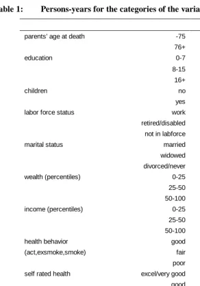
Table 1: Persons-years for the categories of the variables
male female
parents’ age at death -75 11645 15564
76+ 11876 13751
education 0-7 2456 2688
8-15 16312 23249
16+ 4752 3377
children no 1872 3073
yes 21649 26241
labor force status work 6442 3895
retired/disabled 16954 18591
not in labforce 124 6829
marital status married 19263 13953
widowed 2846 12830
divorced/never 1413 2532
wealth (percentiles) 0-25 4600 8721
25-50 5452 7337
50-100 13469 13256
income (percentiles) 0-25 8339 14480
25-50 5940 6645
50-100 9242 8189
health behavior good 2466 4987
(act,exsmoke,smoke) fair 9356 15558
poor 11699 8770
self rated health excel/very good 8694 10638
good 7536 8854
fair 4823 6372
poor 2468 3450
objective health excel/very good 16663 18603
(hospital,adl,thin,loss) good 5095 7713
fair 1450 2502
poor 313 497
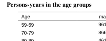
Table 2: Persons-years in the age groups
Age male female
59-69 9612 8044
70-79 8668 11775
80-89 4618 7934
90+ 623 1562
sum: 23521 29315
4. Methods
I apply event-history-analysis with a model for the force of mortality as the outcome variable. The models include a baseline for the basic time variable age that is piecewise linear and coefficients for the multiplicative impact of categorical variables on the baseline risk of dying. The risks are computed as rates, based on occurrences (deaths) and exposures (persons-months) for specific combinations of variable levels. The results are displayed as rate ratios. I used STATA 8 and aML 2.04. The baseline for age covers the age range from 59 to 107 whereas the observation period is only 8 years, namely from 1992 to 2000. Thus, the cohorts are not real cohorts but partly synthetic ones in the sense that in spite of the longitudinal data, no individual in the data set is really observed from age 59 to ages above 67.
The analysis of selective mortality is limited by the fact that only persons who survived until age 59 are included in the study. Persons who entered the study after age 59 are left-truncated, i.e. we only consider the period at risk after the respondents have entered the sample. STATA allows taking into account left-truncated cases by distinguishing between “time under risk” and “time under observation”.
Different models are used in different steps to draw conclusions about the causal relationships between the predictor variables and their impact on mortality. Relative mortality rates are computed using different interactions and a term for unobserved heterogeneity. The general formula for the model is:
i m l m l lm k ik k ij j j
variable, A and B, where I is an indicator that equals 1 for a specific combination of the levels of the two variables and that equals 0 otherwise. U stands for a heterogeneity term that is assumed to measure an individually constant frailty in the sample. The mean and the variance of U in the population are assumed to decrease with age because mortality selection makes the population more homogeneous.
5. Results
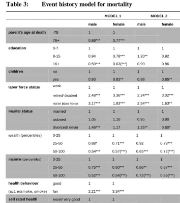
Table 1 shows the relative risks of dying. The underlying models are without interactions and separate for men and women. The absolute baseline risk for the four age groups is not shown. The baseline risk roughly doubles from one age group to the next, i.e. with every ten years of age. The mean age at death is 79 for males and 84 for females.
Model 1 only contains the univariate results of each variable separately. All variables show the expected association with mortality and all of them are significant, except marital status for women and having children for men. Surprisingly, men with 8 to 15 years of education do not have a significantly lower mortality compared to those with 0 to 7 years of education.
Table 3: Event history model for mortality
MODEL 1 MODEL 2 MODEL 3
male female male female male female
parent's age at death -75 1 1 1 1
76+ 0.86*** 0.77*** 0.92 0.87**
education 0-7 1 1 1 1 1 1
8-15 0.94 0.78*** 1.20** 0.92 1.37*** 1.03 16+ 0.59*** 0.63(***) 0.99 0.86 1.31(**) 0.94
children no 1 1 1 1 1 1
yes 0.93 0.83** 0.98 0.85** 0.99 0.87*
labor force status work 1 1 1 1 1 1
retired/ disabled 2.48*** 3.36*** 2.24*** 3.02*** 1.54*** 2.17*** not in labor force 3.17*** 1.83*** 2.54*** 1.63** 1.97** 1.20
marital status married 1 1 1 1 1 1
widowed 1.05 1.10 0.95 0.90 1.01 0.91 divorced/ never 1.46*** 1.17 1.25** 0.80* 1.22* 0.77**
wealth (percentiles) 0-25 1 1 1 1 1 1
25-50 0.88* 0.71*** 0.92 0.78*** 1.05 0.91 50-100 0.54*** 0.57(***) 0.65*** 0.72(***) 0.87(*) 0.90
income (percentiles) 0-25 1 1 1 1 1 1
25-50 0.75*** 0.60*** 0.86** 0.67*** 0.95 0.75*** 50-100 0.52*** 0.54(***) 0.72(***) 0.65(***) 0.82(**) 0.74(***)
health behaviour good 1 1 1 1
(act, exsmoke, smoke) fair 2.21*** 3.34*** 1.73*** 2.40***
self rated health excel/ very good 1 1 1 1
good 1.58*** 1.65*** 1.32*** 1.44***
fair 2.60*** 2.68*** 1.85(***) 1.92(***) poor 6.11*** 4.52*** 3.38*** 2.6(***)
objective health excel/ very good 1 1 1 1
(Hospital,adl, thin, loss) good 2.08*** 1.76*** 1.36*** 1.22*** fair 3.56(***) 3.43*** 1.74(***) 1.98*** poor 5.03(***) 4.77(***) 2.27(***) 2.39(***)
Widows do not display a significantly different mortality from married persons. Men who are divorced or who have never married have a higher mortality whereas women in the same group have a lower one. Interestingly, the relative mortality risk of divorced or never married women turned from an insignificantly higher mortality according to the univariate results of Model 1 to a significantly lower mortality risk in Model 2 (see discussion).
Finally, income and wealth both have a strong diminishing impact on mortality. One intermediate step between Model 2 and 3 is not shown here: it adds only health behavior to the SES variables and shows that the measured items of health behavior (physical activity, being an ex-smoker and being a smoker) changes the coefficients only slightly and do not remove the significance of any socioeconomic variables. This means that socioeconomic mortality differences to a large extent can not be explained by physical activity or smoking.
Model 3 is the full model, where the three health variables and also parents’ mean age at death are added. We see that a high parents’ mean age at death significantly reduces the mortality of women, and this supports the assumption that common genes in a family contribute to longevity. This interpretation is likely to be true, not least because the inclusion of parents’ education in the model as an indicator of their social status does not change the impact of their age at death (results not shown). Thus, in Model 3 parents’ SES is not a common background factor influencing both the parents’ mean age at death and the mortality of the respondent. The genetic explanation is less likely if one assumes that parental education is not a good indicator for childhood conditions or if intergenerational continuities like smoking are more important than genes.
In the full model, wealth is no longer significant but most of the other socioeconomic mortality predictors still are. This indicates that the transition from a given health status to death is also influenced by SES. In the modeling of complex processes like those between SES, health and mortality, it is likely that some of the variables are intermediate variables for others and that they are not independent from each other. In this study, I find the highest correlations between wealth and income (r= 0.47) and between wealth and education (r= 0.40). As to the health variables, there are very low correlations between objective health and health behavior (men: 0.09, women 0.16), low correlations between health behavior and self-rated health (0.22 and 0.14) and strong correlations between self-rated health and objective health (0.39 and 0.44). For SES as for health, it is clear that we have to measure multiple interrelated dimensions. This is justified as long as the different variables reveal interesting differences in their model results and these results are interpreted with caution.
range and across all levels of different other variables. This assumption is too simplistic. Therefore, the following interactions give a more accurate picture of the influence of selected variables.
Figure 1: Female mortality with interaction between education and wealth (based on Model 2, low education and low wealth = 1)
0 0.2 0.4 0.6 0.8 1 1.2 1.4
0-25% 25-50% 50-100% 0-7y
8-15y 16+y
re
la
ti
v
e
m
o
rt
al
it
y
wealth percentile
An interaction between education and wealth (Figure 1) shows that for women material wealth is only beneficial when combined with middle or higher education and higher education is beneficial only in combination with at least average wealth. When I use income instead of wealth in such a graph, the result is similar. This means that beyond the result of Model 2, where the financial variables removed the positive influence of higher education, we now see that for women these two different resources have a complementary impact on mortality, i.e. both are necessary to have a mortality advantage.
wealthier persons and also when we compare wealth groups within the higher educated group.
The corresponding graph for males is not shown and discussed here. This is because it shows a different pattern, which is dominated by the surprising excess mortality of men with intermediate education. Since I do not know the reason for this mortality pattern (see discussion), an interaction between education and wealth for men would not provide deeper insights.
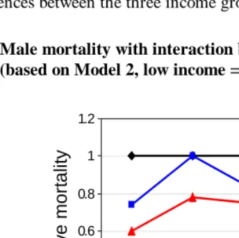
To address my central question, i.e. whether socioeconomic mortality differences are stable or declining with increasing age, it is necessary to run interactions between age, i.e. the basic time variable of the model, and a variable for SES. In the following analysis, I will use income as an indicator for SES. This is because it has the highest independent impact on mortality (see Table 1). In order to limit the material in this article, the following figures show mortality patterns for men. Women show neither more nor less convergence with age, but generally have an even less clear pattern over age than men.
Figure 2 shows the mortality for men with interaction between age and income. Note that the graph does not show the increase of mortality with age but only the relative differences between the three income groups.
Figure 2: Male mortality with interaction between age and income (based on Model 2, low income = 1)
0 0.2 0.4 0.6 0.8 1 1.2
59-69 70-79 80-89 90+
0-25%
25-50%
50-100%
relat
iv
e
m
o
rt
alit
y
As we saw in Table 1, men with the highest income have a significantly lower mortality. The upper bound of the confidence interval for the richest group (red line) for the four age groups is 0.84, 0.99, 0.95 and 1.16. The confidence interval for the oldest group is wider because of low case numbers in this group. Those with a middle income also display a lower mortality, but this is not significant at the 5 per cent level. Far from significant in this graph are the fluctuations of differences over age groups. This suggests that mortality differences between income groups are relatively stable over age and obviously not declining with increasing age. Again, the level of significance is not satisfactory, but here the differences in the oldest age group are non-significant because of the wide confidence interval due to low case numbers rather than because of a mortality convergence in old age.
Figure 3 repeats Figure 2 (thin lines) and shows the same interaction but based on Model 3, which controls for the health variables (thick lines).
Figure 3: Male mortality with interaction between age and income (based on Model 3, health controlled (HC), low income = 1)
0 0.2 0.4 0.6 0.8 1 1.2
59-69 70-79 80-89 90+
0-25% 25-50% 50-100% 25-50%HC 50-100%HC
re
la
ti
ve
mo
rt
a
lit
y
age
The next step is to address the problem of heterogeneity. Unfortunately, the model represented by the equation above, which includes the heterogeneity term U, did not show the expected results. Neither aML nor STATA 8 was able to identify heterogeneity in the estimation procedure. This is most likely due to the sample size, an insufficient observation time or insufficient variation in time varying variables and not to the absence of heterogeneity in the sample because even in models with very few variables heterogeneity was not found.
The assumption is that after controlling for heterogeneity, the relative risks would show a more realistic picture of determinants for individual mortality. The mortality differences between social groups as shown in Figure 2 and 3 are likely to be underestimated in higher ages because the population at high ages is more homogenous due to selective mortality. Thus, the true change of the impact of income over age for the individual can only be shown after a successful estimation of heterogeneity that in this case has to be postponed until better data are available. But since it is known in what direction the heterogeneity bias works, it is possible to conclude from the results so far that the impact of SES is not decreasing with rising
age.
The next step shows how a health decline is affecting the impact of social status on mortality. Figure 4 shows an interaction between self-rated health and income. Age is still controlled for with four age groups, as it is in all models.
Figure 4: Male mortality with interaction between income and health (based on Model 3, low income = 1)
0 0.2 0.4 0.6 0.8 1 1.2
very good good fair poor 0-25%
25-50%
50-100%
self-rated health
re
la
ti
ve
mo
rt
a
lit
This interaction shows that income matters a lot when the person is in good health and that it has no impact when the person is in poor health. This means that poor health levels socioeconomic mortality differences. The mortality difference between the lowest and the other income groups is only significant at the 5 per cent level when people are in good health (RR: 0.45, CI: 0.32-0.62; RR: 0.69, CI: 0.47-0.95).
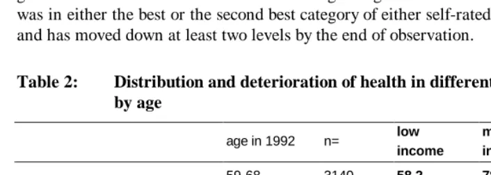
If the health status is so important for the impact of SES on mortality, then the resulting question is whether the health decline with age is equally distributed between social groups, enough to result in a leveling of the mortality between social groups. I would like to report here three aspects of health distribution. First, health declines generally with age: The correlation between age and average health during the study is 0.20*** for self-rated health and 0.34*** for objective health. There seems to be an adjustment for age in the self-estimation of health, which results in a lower correlation with age compared to the objective measure. But despite of the general health decrease with increasing age, health is unequally distributed between income groups: Table 2 shows the other two aspects of the health distribution: first, the average self-rated health status at the beginning of the observation and, second, the experience of a health deterioration, both by the three income groups from above. A transition from good to bad health here means that at the beginning of the observation period a person was in either the best or the second best category of either self-rated or objective health and has moved down at least two levels by the end of observation.
Table 2: Distribution and deterioration of health in different income groups by age
age in 1992 n= low
income
middle income
high income
59-68 3140 58.2 78.4 88.7
69-78 4114 54.9 74.9 80.6
Percentage having very good or good health at the beginning of observation
79-102 2122 52.6 69.8 73.3
59-68 2408 13.1 9.6 6.5
69-78 2799 18.1 13.7 11.8
Percentage that experiences a health deterioration
It is difficult to measure how large health differences are and even more so to measure how these differences change with age. But it is obvious that even if health generally declines with age, people with lower income initially have a lower health status and are more likely to experience a health decline. The number of cases for the analysis of health decline is smaller than that for the analysis of health at onset because only healthy persons can be considered for a possible health decline. In the oldest age group (the last row of the table), healthy persons are especially rare and selected, which may explain that the differences are not significant.
Concerning the question whether socioeconomic mortality differences decline with age or not, it is, finally, important to see whether the impact of the health status on mortality is stable across age groups. Figure 5 shows the interaction between age and health.
Figure 5: Male mortality with interaction between age and self-rated health (based on Model 3, very good health = 1)
re
la
ti
v
e
m
o
rt
a
lit
y
age
0 1 2 3 4 5 6 7
59-69 70-79 80-89 90+ very good good f air poor
same interactions based on the objective health measure show an even stronger convergence (results not shown). Note that, naturally, it is possible to represent the interaction in Figure 5 in absolute terms. Mortality then would increase strongly with age and the distance between the lines, i.e. the absolute differences in the mortality risk, would only slightly decrease with age. But since I do not focus on the general increase in mortality with age, the chosen representation in Figure 5 is more appropriate.
The main result with respect to the convergence of socioeconomic mortality differences is that these differences are stable across age. However, they converge as health deteriorates. But health, in turn, assumes less importance for mortality in old age.
6. Discussion
6.1 Excess mortality of men with intermediate education
The surprisingly higher mortality for men with an intermediate education has been observed also elsewhere (e.g. Liang et al. 2002) and it has been interpreted as an educational mortality crossover due to selective mortality. An alternative explanation is that, holding income constant in the model, higher education means that the aforementioned education is not translated into higher income. This could be because the person never obtained a job that matches the educational level or he lost his job and thus experienced downward mobility, a move that may have been health related. This interpretation is supported by the fact that the excess mortality for middle educated men concentrates on the lower income and poorer health groups (results not shown). It also supports that education is not beneficial on its own but only when combined with higher income. This has been shown for women in Figure 1. One possible conclusion is that education as a measurement of SES has, besides several advantages, the disadvantage of being too stable across the life course.
6.2 Disadvantage for married women?
does not allow for a detailed discussion of the reasons. But the fact that the sex difference emerges only after controlling for income and wealth may indicate that married women profit from higher material resources. Besides, they do not have an advantage or may even have a disadvantage when married net of the other factors in my analysis. Grundy and Slogett (2003) argued that women experience less of a disadvantage of being single than men because they engage less in unhealthy behavior in such situations (Johnson et al. 2000) and are more likely to substitute their singlehood with social networks (Goldman et al. 1995). In addition, they may even suffer in marriage, where they are likely to be the younger and healthier partner whose role it is to care for the ill spouse (Beckett et al. 2002).
6.3 Education and wealth work together to lower mortality
The interaction between education and wealth shows that for women neither education nor material wealth is beneficial separately (Figure 1). The excess mortality of women with high education but a low wealth status can be understood when we consider education as input and wealth as an output of the labor market. This group may suffer from not being successful in translating their education into material wealth or they lost their original occupational status. This would simply indicate that material wealth is a stronger mortality predictor than education. The other group with higher mortality, women with low education and a high wealth status, seems to indicate that this is not a general rule. Besides the order of importance between these dimensions of SES, there is a disadvantage of persons with an inconsistent social status, which means being on different levels in different dimensions of the social status (Siegrist et al. 1990). As indicated above, it was not possible to find or to reject this pattern for men because of the surprising higher mortality of men with an intermediate education, which makes the corresponding Figure for men difficult to compare to Figure 1.
6.4 SES mortality differences converge with declining health but not with age
The main result from the previous section, the convergence of socioeconomic mortality differences with worsening health but not with age, questions the majority of studies that do not separate age and health decline and find socioeconomic mortality differentials that converge with age.
The equalizing effect of worse health does not mean that social inequalities no
longer exist after health has become poor. It rather raises the question to what extent
in a more or less severe health decline and that, therefore, there is no longer social inequality in the transition from poor health to death. Thus, the question of social inequality in health is analogous to and becomes part of the question of social inequality in mortality.
Research findings reveal clear socioeconomic health differences at old age (e.g. Huisman et al. 2003) but the question of convergence or divergence with age is as unclear for health differences as it is for mortality differences. The majority of research results show converging health differences with age. Ross and Wu (1996) show that health differences increase up to age 90 and Huisman et al. (2003) more often find converging patterns but also mixed evidence depending on sex, country and indicator for SES. They studied socioeconomic inequalities in morbidity, using very good data from 11 European countries and find that morbidity differentials decrease with age in most countries but are stable and also increase in others. The convergence is less consistent for men than for women and less consistent for education as indicator for SES compared to income. The authors state that a small part of the observed convergence can be attributed to a bias caused by institutionalized persons, which have been excluded from their data. Concerning the obvious international differences, they assume that concrete risk factors, like drinking and smoking, may be responsible. Depending on the country, they may or may not cause a mortality convergence because such behavior is more common in lower status groups (which increases the gradient) and less common so among old people (resulting in a convergence with age).
In my study, I could only make an attempt to analyze health inequalities, which reveals increasing health differences because, from an already unequally distributed health at onset, the rate for health deterioration is also higher for low income groups (see Table 2 and Figure 6 below).
A closer look at Figure 3 shows that controlling for health decreases mortality differences in early old age. This is not surprising, since health is an intermediate variable and its inclusion in the model should, as observed in Model 3 in Table 1, decrease social mortality differences. The question arises why this inclusion does not change mortality differences in old age. A possible answer is provided in Figure 5: if the health status is less important for mortality in old age, controlling for health should accordingly change social mortality differences less so than in younger age groups.
and that instead of age, poor health is the equalizer for social differences, maybe as a result of a universal shift from social to biological determinants of mortality when health decreases (argument 1). The arguments mentioned seem to be not mutually exclusive, e.g. accumulating social differences and the dominance of bad physical conditions over social conditions are possibly simultaneous.
The central question of my research, i.e. whether socioeconomic mortality differences decrease with age or not, has been answered by a modification of the question, namely the identification of two aspects of increasing age. Both of these aspects increase mortality but have very different implications for the impact of SES on mortality. The first aspect, increasing numerical age, seems to be trivial but, in fact, some of the arguments used to support the hypothesis of mortality convergence are based on numerical age. These arguments can now be rejected. The second aspect is declining health, where my finding that money matters less in poor health rejects the assumption that money is of major importance to people in bad health to get good treatment to prevent them from dying. Concerning declining health, the problem remains: the theoretically simple scenario that a socially mixed sample will experience a simultaneous health decline that would level social differences in mortality will practically never happen. The health decline of upper class persons will either be delayed, will start on a higher health level or will be slower. Therefore, it is difficult to say if the potentially leveling impact of a health decline is actually effective. This is because poor health is likely to be to a large extent the result of low SES and thus it is unequally distributed.
Figure 6: Transitions between good health and death
poor health good health
death
higher rates
for low SES
A
C B
higher rates for low SES
no difference between SES
It is not obvious from my findings, how age is intervening in this constellation. On the one hand, Figures 2 and 3 show that the impact of social status is constant, on the other hand, the impact of health on mortality decreases with age (Figure 5). To answer this question, a very good measurement of socioeconomic health differences across age groups and maybe a multi-process model would be advantageous, but both go beyond the scope of this study at the present stage.
Reference list
Adams Peter, Hurd Michael D, Mcfadden Daniel, Marrill Angela, Ribeiro Tiago. (2002). "Healthy, wealthy, and wise? Tests for direct causal paths between health and socioeconomic status." Journal of Econometrics, 112, 1:3-56.
Auerbach James A, Krimgold Barbara K. (2001). Income, Socioeconomic Status and Health: Exploring the Relationship. NPA Report, Washington, DC: National Policy Association et al.
Beckett Megan, Goldman Noreen, Weinstein Maxine, Lin I-Fen, Chuang Yi-Li. (2002). "Social environment, life challenge, and health among the elderly in Taiwan." Social Science and Medicine, 55, 191-209.
Beckett Megan. (2000). "Converging health inequalities in later life - an artifact of mortality?" Journal of Health and Social Behaviour, 41:106-119.
Breeze Elizabeth. (2000). Health inequalities persist into old age: results from the longitudinal study. In: Butler RN, Jasmin C. Longevity and Quality of Life:
Opportunities and Challenges. New York et al.: Kluwer Academic Press /
Plenum Publishers: 171-179.
Crystal Stephen, Shea Dennis. (1990). "Cumulative advantage, cumulative disadvantage, and inequality among elderly people." The Gerontologist, 30, 4: 437-443.
Dannefer Dale. (2003). "Cumulative Advantage/Disadvantage and the Life Course: Cross-Fertilizing Age and Social Science Theory." Journal of Gerontology:
Social Sciences, 58B, 6:327-337.
Davey Smith George, Gunnell David, Ben-Shlomo Yoav. (2001). Life-course approaches to socio-sconomic differentials in cause-specific mortality. In: Leon DA, Walt G. Poverty, Inequality and Health: an International Perspective. Oxford: Oxford University Press: 88-124.
Doblhammer Gabriele. (2000). "Reproductive History and Mortality Later in Life: A Comparative Study of England & Wales and Austria." Population Studies, 54, 2: 169-176.
Fox Anthony J, Goldblatt Peter O, Jones D R. (1985). "Social Class Mortality Differentials: Artefact, Selection or Life Circumstances?" Journal of
Epidemiology & Community Health, 39:1-8.
Goldman Noreen, Korenman Sanders, Weinstein Rachel. (1995). "Marital status and health among the elderly." Social Science and Medicine, 40, 1717-1730.
Goldman Noreen. (2001). "Social Inequalities in Health: Disentangling the Underlying Mechanisms." Annals of the New York Academy of Sciences, December (954):118-39.
Greenberg James A. (2001). "Biases in the Mortality Risk Versus Body Mass Index Relationship in the NHANES-1 Epidemiologic Follow-Up Study." International
Journal of Obesity, 25:1071-78.
Grundy Emily, Sloggett Andy. (2003). "Health inequalities in the older Population: the role of personal capital, social resources and socio-economic circumstances."
Social Science and Medicine, 56, 935-947.
Himes Christine. (2000). "Obesity, Disease, and Functional Limitation in Later Life."
Demography, 37(1):73-82.
Hoem Jan M. (1989). The Issue of Weights in Panel Surveys of Individual Behavior. In: Panel Surveys. Stockholm Research Reports in Demography, 39:539-65.
House James S, Kessler Ronald C, Herzog A Regula. (1994). "The social stratification of aging and health." Journal of Health and Social Behaviour, 35:213-234.
Huisman Martijn, Kunst Anton E, Mackenbach Johan P. (2003). "Socioeconomic inequalities in morbidity among the elderly; a European overview." Social
Science and Medicine, 57:861-873.
Huisman Martin, Kunst Anton E, Andersen Otto, Bopp M, Borgan J-K, Borrell C, Costa G, Deboosere P, Desplanques G, Donkin A, Gadeyne S, Minder C, Regidor E, Spadea T, Valkonen T, Mackenbach J-P. (2004). "Socioeconomic Inequalities in Mortality Among Elderly People in 11 European Populations."
Journal of Epidemiology & Community Health, 58(6):468-75.
Johnson Norman J., Backlund Eric, Sorlie Paul D., Loveless, Catherine A. (2000). "Marital status and mortality: The National Longitudinal Mortality Study."
Liang Jersey, Bennet Joan, Krause Neal, Kobayashi Erika, Kim Hyekyung, Brown J. Winchester, Akiyama Hiroko, Sugisawa Hidehiro, Jain Arvind. (2002). "Old age mortality in Japan: Does the socioeconomic gradient interact with gender and age?" Journal of Gerontology: Social Sciences, 57b:294-307.
Lillard Lee A., Panis Constantijn W A. (2003). "aML Multilevel Multiprocess Statistical Software Version 2.04." Los Angeles, California: Econware (http://www.applied-ml.com).
Losonczy Katalin G, Harris Tamara B, Cornoni-Huntley Joan, Simonsick Eleanor M, Wallace Robert B, Cook Nancy R, Ostfeld Adrian M, Blazer Dan G. (1995). "Does Weight Loss From Middle Age to Old Age Explain the Inverse Weight Mortality Relation in Old Age?" American Journal of Epidemiology, 141(4):312-21.
Mackenbach Johan P, Kunst Anton E, Valkonen Tapani. (1999). "Socioeconomic inequalities in mortality among women and among men: An international study." American Journal of Public Health, 89:1800-1806.
Marmot Michael G, Shipley Martin J. (1996). "Do socioeconomic differences in mortality persist after retirement? 25 year follow up of civil servants from the first Whitehall study." British Medical Journal, 313: 1177-1180.
McCord Colin, Freeman Harold P. (1990). "Excess Mortality in Harlem." New
England Journal of Medicine, 322:173-7.
O'Rand Angela M. (1996). "The Precious and the Precocious: Understanding Cumulative Disadvantage and Cumulative Advantage Over the Life Course."
The Gerontologist, 36:230-238.
Otterblad Olausson Petra. (1991). "Mortality Among the Elderly in Sweden by Social Class." Social Science and Medicine, 32:437-40.
Pappas Gregory, Queen Susan, Hadden Wilbur, Fisher Gail. (1993). "The Increasing Disparity in Mortality Between Socioeconomic Groups in the US, 1960 and 1986." New England Journal of Medicine, 329(2):103-9.
Preston Samuel H, Elo Irma T. (1995). "Are educational differences in adult mortality increasing in the United States?" Journal of Aging and Health, 7:476-496.
Reuben David B, Rubenstein Lisa V, Hirsch Susan H. (1992). "Value of Functional Status as a Predictor of Mortality: Results of a Prospective Study." American
Ross Catherine E, Wu Chia-Ling. (1996). "Education, age, and the cumulative advantage in health." Journal of Health and Social Behaviour, 37:104-120.
Schrijvers Carola T M, Stronks Karien, van de Mheen H Dike, Mackenbach Johan P. "Explaining educational differences in mortality: the role of behavioral and material factors." American Journal of Public Health, 89(4):535-540.
Siegrist Johannes, Peter Richard, Junge Astrid, Cremer Peter, Seidel Dieter. (1990). "Low Status Control, High Effort at Work and Ischemic Heart Disease: Prospective Evidence from Blue-Collar Men." Social Science and Medicine, 31(10):1127-34.
Smith James P, Kington Raynard S. (1997). Race, socioeconomic status and health in late life. In: Martin LG, Soldo BJ. Racial and Ethnic Differences in the Health
of Older Americans. Washington: National Research Council: 105-162.
Smith James P. (2004). "Unravelling the SES health connection." IFS Working Papers W04/02, Institute for Fiscal Studies.
Smith James P. (2003). "Consequences and Predictors of New Health Events." NBER Working Papers 10063, National Bureau of Economic Research, Inc.
Smith James P. (1999). "Healthy Bodies and Thick Wallets: the Dual Relation between Health and Economic Status." Journal of Economic Perspectives, 13(2):145-66.
Soldo Beth J, Hurd Michael D, Rodgers Willard L, Wallace Robert B. (1997). "Assets and health dynamics among the oldest old: an overview of the AHEAD study."
The Journals of Gerontology, 52b, Special Issue: 1-20.
StataCorp (2003). Stata Statistical Software: Release 8.0. College Station, TX: Stata Corportation (http://www.stata.com).
Stronks Karien. (1997). Socio-Economic Inequalities in Health: Individual Choice or Social Circumstances? Dissertation. Rotterdam. Erasmus University.
Valkonen Tapani. (2001). "Life Expectancy and Adult Mortality in Industrialized Countries." International Encyclopedia of Social and Behavioral Sciences. 8822-8827.
Warren John R, Kuo Hsiang-Hui. (2003). "How to Measure 'What People do for a Living' in Research on the Socioeconomic Correlates of Health." Annals of