journal homepage: http://jac.ut.ac.ir
Optimization of profit and customer satisfaction
in combinatorial production and purchase model
by genetic algorithm
Fatemeh Ganji
∗1and Zahrasadat Zamani
†21,2
Department of Industrial Engineering, Gopayegan University of Technology, Golpayegan, Iran.
ABSTRACT ARTICLE INFO
Optimization of inventory costs is the most important goal in industries. But in many models, the constraints are considered simple and relaxed. Some actual con-straints are to consider the combinatorial production and purchase models in multi-products environment. The purpose of this article is to improve the efficiency of inventory management and find the economic order quantity and economic production quantity that can minimize the cost of inventory and customer satisfac-tion. In this study, the models with these targets in combinatorial production and purchase systems with the assumption the warehouse and budget constraints are proposed. Since a long time for solving the problem with an exact method is required, we develop a genetic algorithm. To evaluate the efficiency of the proposed
Article history:
Received 10, June 2018
Received in revised form 19, April 2019
Accepted 27 May 2019
Available online 01, June 2019
Keyword: combinatorial production and purchase model; ge-netic algorithm; inventory control.
AMS subject Classification: 05C78.
∗Corresponding author: F. Ganji. Email: [email protected] †[email protected]
1
Abstract continued
algorithm, test problems with different sizes of the problem in the range from 1 to 2000 jobs, are generated. The results show that the genetic method is efficient to determine economic order quantity and economic production quantities. The computational results demonstrate that the average error of the solution is 10.93%. (FITNESS AND TAGUCHI)
2
Introduction
[9] added partial backordering to the basic EPQ model (EPQ-PBO). Although a comprehensive review of deterministic partial backordering models is proposed by Pentico and Drake [11]. They studied more complicated model structures, partial backordering models that include either time-based backordering rate functions or additional considerations. A model for the EPQ-PBO in which the constant backordering rate changes when production starts is studied by them [11].
Stockton and Quinn [13] considered the basic EOQ model using Genetic Algo-rithms to solve economic lot size. This model is based on a deterministic policy such as constant demand and repetitive replenishment, in which backorder is not allowed. Besides, Hou et al. [7] also applied the periodic review method in produc-tion inventory management using Genetic Algorithms approach. In that model, they assume that backorders are allowed and the demand is constant. Further-more, [1] demonstrated the use of a periodic review model by determining the fixed order quantity in periodic review approach. Ghodsypour and O’Brien [2] developed an integer non-linear programming model which consider the total cost of inventory, including total price, shortage, and transportation and ordering cost. Yokoyama [16] proposed a model for a multiple sourcing inventory and distribution system. That model focused on finding the target inventory and transportation quantity that minimizing the total cost of the system by using a random local search method combined with GAs.
In the present work, Genetic Algorithms are applied to find out optimal solutions through the optimization process. Our aim is to find an optimal ordering quantity for various inventory items stored.
Also, the single machine scheduling problem with one flexible maintenance period and non-resumable jobs are considered by minimizing the weighted number of tardy jobs. It is assumed that there is a flexible maintenance period that its starting time is as the decision variable. Moreover, the idle time is not allowed. The rest of this paper is organized as follows: the problem is described in Section 3. Notation and mathematical model is presented in Section 4. Section 5 is aimed at proposing a heuristic algorithm. Computational experiments are then given in Section 6 to demonstrate the effectiveness of algorithm, followed by the conclusion in Section 7.
3
Preliminary
management strategy.
• Perpetual Inventory: Perpetual inventory is a method of accounting for in-ventory that records the sale or purchase of inin-ventory immediately through the use of computerized point-of-sale systems and enterprise asset manage-ment software. The perpetual inventory provides a highly detailed view of changes in inventory with immediate reporting of the amount of inventory in stock, and accurately reflects the level of goods on hand.
• Purchase Order Lead Time: Purchase order lead time is the number of days from when a company places an order for production inputs it needs to when those items arrive at the manufacturing plant. Purchase order lead times vary from company to company and from industry to industry, depending on the types of goods or materials being ordered, their relative abundance or scarcity, where the suppliers are located, and even the time of year.
• Back Order: A backorder is a customer order that has not been fulfilled. A backorder generally indicates that customer demand for a product or service exceeds a company’s capacity to supply it.
In many studies in inventory control purchase models and production, models are considered separately with regard to special assumption, but in a real environment, it is important to consider two scenarios together. In this article the combinato-rial EOQ and EPQ model considering multi products and budget and warehouse space constraints. The shortage is permitted such as backordering. The aim of this research is to minimize the bi-criteria targets, inventory cost, and customers satisfaction. The purpose of this article is to improve the efficiency of inventory management and find the economic order quantity and economic production quan-tity that can minimize the cost of inventory and customer satisfaction. the model with these targets in combinatorial production and purchase systems with the as-sumption the warehouse and budget constraints in multi products environment is developed. It is assumed that if the shortage gets to a specific level, the new order is performed. Before the model’s description, there are some assumptions that we need to define in this research.
• Annual demand is constant
• Lead times are known and constant
• Backorders are allowed
• On hand inventory at the end of the starting period is zero.
• Purchasing cost is less than the shortage cost.
4
Notations and mathematical modeling
In this section, we define notations and decision variables to model the problem. Then a mathematical model is proposed. The following notations are used in this section:
Problem parameters:
• Di: demand rate of product i
• Pi: production rate of product i
• Si: shortage value of product i
• hi: holding cost of product i per time unit
• fi: required space for product i
• X: maximum budget
• A1i: ordering cost of product i per order
• A2i: production cost of product i per order
• π1i: shortage cost per unit product i independent unit time
• π2i: shortage cost per unit product i per unit time
• F: total space of the warehouse
• C1i: purchase cost of producti
• C2i: production cost of product i
• Ri: sales price of product i
Decision variables:
• T IC: inventory cost
• T HCi: total holding cost of product i
• T SCi: total shortage cost of product i
• T M Ci: total purchasing cost of product i
• T OCi: total ordering cost of product i
• Ti: cycle length of product i
• Q1i: optimal order value of product i
• Q2i: optimal production value of producti
• Ei: start point of producti
The mathematical model
The inventories costs are obtained from the summation of holding, ordering, pur-chasing, and production costs and cost of shortage. By considering the assumptions mentioned in the previous section, the component of inventory costs are calculated as follows:
T IC =
N X
i=1
(T HCi+T SCi+T M Ci+T OCi).
Calculation of total holding cost: total holding costs are calculated by the following relation:
T HCi = hi
2[
(Q1i+Ei)2 Di
+ E
2 i Di−Pi
]1
Ti .
Calculation of total cost of shortage: for calculating the total cost of shortage, we must sum two related costs such as dependent to unit time and independent one. Therefore, it is obtained by the following equation:
T SCi = [π1iSi+π2i( S2
i
(Di−Pi)2)]
1
Ti.
T M Ci = (C1iQ1i+C2i+Q2i)
1
Ti .
Calculation of total ordering cost: total ordering costs is calculated by the following relation:
T OCi = (A1i+A2i)
1
Ti.
Calculation of total revenue: total revenue of products sales is obtained as follows:
N X
i=1 RiDi.
Constraints: the constraints of budget and warehouse space are calculated as the following relations respectively:
N X
i=1
C1iQ1i+C2iQ2i ≤X and N X
i=1
fiQ1i ≤F.
Satisfaction of customer: the customer’s satisfaction in this study, is calculated as follows:
N X
i=1
Di Q1i+Q2i
.
According to above explanation about component of the mathematical model, the inventory model is obtained as follows:
maxZ1 :
N X
j=1
RiDi−
Di(Di−Pi) Pi(Ei−Q1i) +ziDi
[(A1i+A2i)+(C1iQ1i+C2iQ2i)+
hi
2[
(Q1i+Ei)2 Di
+ E
2 i Di−Pi
]1
Ti
+ [π1iSi +π2i( S2
i
(Di−Pi)2
)]1
Ti
] (1)
maxZ2 :
N X
i=1
Di Q1i+Q2i
st:
PN
i=1C1iQ1i+C2iQ2i ≤X i= 1,2, . . . , N
(3)
PN
i=1fiQ1i ≤F i= 1,2, . . . , N
(4)
Q1i ≤Ei i= 1,2, . . . , N
(5) The objective function (1) maximizes the total benefit of inventory. The objective function in relation (2) maximizes the satisfaction of the customer. Constraint (3) ensure that the total costs of purchase and production of all products are not greater than the total budget in hand. Constraint (4) ensure that the occupied space by-products are not greater than the total space of the warehouse. Con-straint (5) shows that the order quantity of productiis not greater than the point of production of it.
5
solution method
In this study, regarding the bi-criteria objective function, the constraint method is proposed. In this procedure, by recursive stages, the optimal solution is obtained in a long time commonly. Therefore, in this research, the constraints method is applied and after passing a long time (with 3600 seconds constraint), two values are obtained for Z2 as 0.1 and 0.61. For calculating the optimum value of Z1, this problem must be solved in GAMS software with one objective and the obtained values for Z2 as constraints, again. Because of a long time for solving the problem with an exact method and regarding NP-hardness of the problem, in this research, the metaheuristic method, a genetic algorithm, is developed. That model con-centrate on finding the target reorder quantities that minimizing the total cost of inventory and satisfaction of the customer, by using random local search method combined with GAs.
Genetic Algorithm
The genetic procedure begins with an initial set of solution which is called chro-mosome. One of them has some gens which specifies their characteristics. The chromosome forms a matrix with i rows and 6 columns as below shape:
The values of genes demonstrate values of decision variables that getting amount randomly and by these values, the objective function which is called fitness in GAs, is calculated.
population parameters:
The population size of GAs is considered 20 and the iteration as stop condition is 20 after controlling the feasibility of solutions. Furthermore, the mechanism of chromosome selection is a roulette wheel, where the selection was done randomly. The probability of mutation is 0.05 and the strategy of doing mutation is one point. The probability of crossover is 0.7 and its process is replacing two genes together randomly. It is worth noting that one chromosome is not feasible from the point of view constraints, that chromosome is eliminated and a new one is generated.
6
Computational results
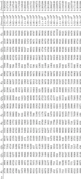
The proposed model is illustrated by considering the following 20 examples(displayed in table 2). In each of examples, 100 independent runs have been performed by the genetic algorithm. So, the best-found values Z1,Z2,Q1,Q2,Si andEi have been
obtained and showed in table 2. The GA parameters that are applied including the population of GA is 20, the probability of crossover is 0.7 and the probability of mutation is 0.05.
7
Conclusion
Acknowledgments
The author is supported by the Department of Industrial Engineering at the Gol-payegan University of Technology and her special thanks go to the Department for providing all necessary facilities available to her for successfully conducting this research.
References
[1] Chiang, C., (2009), A periodic review replenishment model with a refined delivery scenario, International Journal of Production Economics, 118, pp. 253–259.
[2] Ghodsypour, S.H., O’Brien, C.,(2001), The total cost of logistics in supplier selection, under conditions of multiple sourcing, multiple criteria and capacity constraint, Int. J. Production Economics, 73, pp. 15–27.
[3] Harris, F. W., (1913), How Much Stock to Keep on Hand. Factory, The Magazine of Management 10, pp. 240-241 & 281-284.
[4] Haupt, R. L., Haupt, S.E., (1998), Practical Genetic Algorithms, John Willey & Sons, Inc, New York.
[5] Heizer, J. H., Render, B., (1993), Production and Operation Management, Strategies and Tactics, Allyn and Bacon, Boston.
[6] Hill, C.I., (2005), Operations Management, Palgrave Macmillan, Hampshire. [7] Hou, C.I., Lo, C.Y., Leu, J.H. (2007), Use genetic algorithm in production
and inventory strategy, Proceeding of the 2007 IEEE IEEM, pp. 963–967. [8] Kumar, R., (2016), Economic Order Quantity (EOQ) Model, Global Journal
of Finance and Economic Management, 5(1), pp. 1–5.
[9] Mak, K.L., (1982), A production lot size inventory model for deteriorating items, Computer And Industrial Engineering, 6(4), pp. 309–317.
[10] Montgomery, D., Bazaraa, M.S., Keswani, A.k.,(1973), Inventory Models with a Mixture of Backorders and Lost Sales, Naval Research Logistics Quar-terly, 20(2), pp. 255–263.
[12] Starr, M.K., (2007), Foundations of Production & Operations Management, Thomson, USA.
[13] Stockton, D.J., Quinn, L. (1993), Identifying economic order quantities using genetic algorithms, International Journal of Operation & Production Man-agement, 13, pp. 92–103.
[14] Stock, J.R., Lambert, D.M. (2001), Strategic Logistics Management, McGraw-Hill Higher Education, Boston.
[15] Taft, E. W. (1918). The most economical production lot. The Iron Age, 101, 1410–1412.