Optimal Portfolio Allocation based on two Novel Risk Measures and Genetic Algorithm
S. Amir Ghoreishi1 Hamid Khaloozadeh2
Abstract:
The problem of optimal portfolio selection has attracted a great attention in the finance and optimization field. The future stock price should be predicted in an acceptable precision, and a suitable model and criterion for risk and the expected return of the stock portfolio should be proposed in order to solve the optimization problem. In this paper, two new criterions for the risk of stock price prediction has been presented, of which the first one is based on the interval predictions which vary with time and proportional to the uncertainty of stock price data, while the second one is a constant risk term that is proportional to the prediction error variances of the neural networks. A novel cost function has been presented to simultaneously consider the expected returns and risks.
Genetic algorithm has been used to solve this optimization problem. Finally, 18 shares of the Tehran Stock Exchange have been considered to evaluate the performance ofthe proposed risk criterions. Two proposed risk criteria, by the conditional value at risk (CVaR) associated with the same stock. The problem of stock portfolio optimization has been solved for all three situations, and the PI-based risk criteria yielded a better return.
Keywords: Stock Portfolio Optimization; Interval Prediction Neural Networks; Conditional Value at Risk; Risk measure.
1. Introduction
Stock price prediction is a challenging problem, due to many involved factors, including political events, economic conditions, oil and gold prices, traders' expectations and other environmental factors, which can influence stock prices. In addition, the stock price series generally have a noisy, dynamic, non-linear, complex, non-parametric and chaotic nature.
Therefore, stock market forecasting is considered as a challenging task in predicting financial time series. Financial time series exhibits rather complex patterns (trends, sudden changes, and volatility clustering) and such series are often non-stationary, whereby a variable does not have a
1 (Ph.D. Candidate) Faculty of Electrical and Computer Engineering, Science and Research Branch, Islamic Azad
University, Tehran, Iran.
2 (Professor)Industrial Control Center of Excellence (ICCE), Department of Systems and Control, Faculty of
clear tendency to move towards a constant value or a linear trend. Static prediction models, including time series, require a series of basic assumptions for variables (some preconditions are required for conventional statistical prediction models such as specific probability statistical distribution) and produces prediction models based on mathematical equations that are not easily understood by investors [1].
Neural networks are considered as one of the most powerful tools in financial forecasting [2-4]. They have been inspired by nature, and are potentially able to model any complex nonlinear function with desired precision (They are general function approximators) [5]. They do not require any presupposition for the characteristics of the system data [6], and are widely used for modeling, classification, prediction and control [7-9].
Despite such superiorities, neural networks have two disadvantages. The first is a significant reduction in the prediction accuracy when there is a considerable uncertainty in the system data. Therefore, the reliability of predictions also decreases. Since these uncertainties are not predictable with high precision, the accuracy of the output of the neural networks, which is one-dimensional, is faltered. This weakness of the neural networks is due to the production of the mean value of the target function as output [10]. This problem has been investigated in the load forecasting of the distribution network [11-12], predicting the life expectancy of components [13], the predictions needed to provide financial services [14], the predictions needed in water distribution systems [15], transport systems [16-18] and baggage handling systems [19], have similar problems with conventional neural networks.
The second difficulty of the neural networks is that they produce a single point prediction output and do not provide any criterion for measurement of its accuracy. It is crucial to consider the uncertainties in single-value and point predictions in order to improve the prediction accuracy and subsequent decision-making process.
Maximizing returns and minimizing asset risk are the most important goals in the management of the portfolio of capital. According to the theory of mean - variance (MV), Markowitz, an investor seeks to maximize returns for a predetermined level of asset risk or minimize risk for a certain level of returns [31-32].
𝑀𝑎𝑥𝑖𝑚𝑖𝑧𝑒(𝐸𝑥𝑝𝑒𝑐𝑡𝑒𝑑 𝑟𝑒𝑡𝑢𝑟𝑛 − 𝑅𝑖𝑠𝑘) (1)
Any kind of investment is confronted with uncertainties that put the future return of the portfolio at risk. The risk of an asset is due to the return or value of the portfolio of capital which may be less than expected. The mean-risk models were introduced for the first time in the early 1950s to provide practical solutions to the issue of choosing a portfolio of capital. Using these models, the average risk uses only two parameters of average return and risk to describe the distribution [33].
As noted above, stock price prediction and the presentation of a suitable risk model are two important issues that must be addressed before the optimal portfolio selection. This paper has investigated the risk measures. In this regard, two new risk metrics are proposed using MLP neural networks with differential output and interval prediction to model the uncertainty of the expected return on the allocation of capital. The first risk metric is based on the normalized average of square error of the predicted neural network for stock price prediction. In this criterion, it is assumed that the uncertainties uniformly affect the data and are not variable with time. In the second criterion, the width of PIs that are trained with the stock data are used. In this viewpoint, there is no assumption of uniformity for the uncertainty of the data. A novel cost function was presented to simultaneously consider the expected returns and risks. This is solve using Genetic Algorithm by applying step-by-step algorithm to facilitate the solving process.
2. The necessary preparations for PI
In order to achieve PI, the method presented in [34] has been utilized for training the neural network. In this method, which is called the Lower Upper Bound Estimation (LUBE), all efforts are made to avoid using the output derivative of the neural network with respect to its parameters, which, according to [29], can cause inaccuracy in prediction.
In the LUBE method, unlike previous methods, efforts are not made to reduce the sum of squares of error. But obtaining PIs with the minimum possible width and the acceptable level of coverage probability is the main target. A neural network is used to estimate the upper and lower bound for the production of PIs [19]. One of the criteria that plays the most important role in the production of an appropriate PI is the degree of confidence(1 − 𝛼), where(𝛼 < 1). By definition, this is the quantity indicating the percentages of the system output included by PI. Naturally, in the ideal state, α = 0. The degree of confidence is also known by the name of the coverage percentage of PI or PICP. Expressing it mathematically we have [19, 15, and 11]:
𝑃𝐼𝐶𝑃 =1
𝑛∑ 𝑐𝑖 𝑛
𝑖=1 (2)
Where n is the total number of data and 𝑐𝑖 is equal to one if i’th data is
inside the PI band, and it is zero if it is outside of this band.
𝐿(𝑥𝑖) ≤ 𝑦𝑖 ≤ 𝑈(𝑥𝑖) (3)
Note that 𝐿(𝑥𝑖) and 𝑈(𝑥𝑖) are, respectively lower and upper bounds of PI
for i’th data. In Fig. 1, the Pi-based neural network is presented. As noted before, only the PICP reaching one is not a good measure for evaluating the performance of PI. Another important criterion is the PI band being as small as possible. The prediction interval normalized average width (PINAW) can be used for this purpose:
𝑃𝐼𝑁𝐴𝑊 = 1
𝑛𝑅∑ (𝑈𝑖− 𝐿𝑖) 𝑛
𝑖=1 . (4)
Fig. 1. The PI based on neural network
Therefore, the more the value of PINAW the more will be the value of PICP. But since the neural networks are trained using square measures, instead of using the PINAW criterion for producing PI, the Prediction Interval Normalized Root-mean-square Width (PINRW) is used, which is defined as follows:
𝑃𝐼𝑁𝑅𝑊 =1
𝑅√ 1
𝑛∑ (𝑈𝑖− 𝐿𝑖) 2 𝑛
𝑖=1 . (5)
The advantage of PINRW over PINAW is that it gives greater importance to longer-range intervals and as a result, PIs produced with PINRW are expected to be smaller than those produced by PINAW.
As stated, PIs with a higher coverage percentage and lower widths are preferable and on the other hand, increasing the coverage percentage and reducing the width of the PIs is in contradiction with each other and should be a balance between them. Therefore, PI can be modeled by a multi-objective optimization problem:
(Max
𝜔 𝑃𝐼𝐶𝑃) & ( min𝜔 𝑃𝐼𝑁𝑅𝑊) 𝑠. 𝑡. (0 < 𝑃𝐼𝐶𝑃 ≤ 1) & (𝑃𝐼𝑁𝑅𝑊 > 0) (6)
In (6) finding the optimal weights of the neural network (W∗) is in such a Hidden layer
Input 2 Input 1
Input n
Input n-1 Target
Interval prediction Upper bound
way that the maximum PICP and the PINRW are minimized. The solution of (6) is time consuming and even a significant portion of Pareto's answers will not be acceptable, because the overall reliability of PI will be lost if the PICP falls below a certain threshold as stated in [34]. The requirement that the PICP be increased beyond the limits is considered as a requirement and the optimization problem in modified in the following single objective form:
(𝑚𝑖𝑛
𝜔 𝑃𝐼𝑁𝑅𝑊) 𝑠. 𝑡. (𝜇 ≤ 𝑃𝐼𝐶𝑃 ≤ 1) & (𝑃𝐼𝑁𝑅𝑊 > 0) (7)
In (7), finding the optimal weights of the neural network (W∗) is done to
minimize the PINRW. μ is the threshold of minimum acceptable PICP. It should be noted that solving the problem of single-objective optimization is usually simpler than solving a multi-objective problem and requires less time. Afterward, the single-objective optimization problem will be solved by the PSO algorithm.
2.1. LUBE method
The traditional methods for producing neural network based PIs are in two stages [35]:
1- Neural networks similar to point prediction methods are trained to model learning data.
2- Assuming a specific distribution for the data, their mean values and variance are calculated then, according to the method used, the Hessian and Jacobian matrices of the neural network coefficients are also created. Then PIs are made.
These methods suffer from multiple problems in building PIs. For example, the Delta method takes specific assumptions for data distribution and residues. Also, in the process of building PIs, both the Delta and Bayesian methods require the calculation of the Jacobin and Hessian matrices. This may lead to the problems of specificity of matrices and reduced reliability of PIs. Moreover, the calculation of these matrices is tedious and greatly increases the implementation complexity of these methods. The new LUBE method has been introduced in [36] for the first time. This method trains a two-output neural network to build PIs in one step, without any presupposition on data distribution such that, these two outputs are related to the lower and upper bounds of PI. The LUBE algorithm briefly includes the following steps:
network, including the number of hidden layers and the number of neurons in each layer. Test data is also used to measure the performance of the neural network.
(ii) Since the stock market data is not static, they become stationary with differencing. According to the proposed algorithm [37], this act is done only for the output of the neural network.
𝑥𝑡+𝑛= ∆𝑥𝑡+𝑛+ 𝑥𝑡 (8)
In (8), ∆𝑥𝑡+𝑛 is the static data set obtained by differencing.
(iii) At this stage, the optimal structure of the neural network will be determined. Therefore, for each candidate of the neural network structure, the training process is repeated to a certain number limit (in this paper, the training process is repeated 3 times) and using the evaluation data, the PICP and PINRW of each trained network are calculated. Then, the optimal structure of the neural network is selected with a certain criterion. In this paper, contrary to [34], a neural network is chosen with a larger cost function J. Where J of each candidate of the neural network is the mean of the 3 neural networks cost functions.
𝐽 = 𝑃𝐼𝐶𝑃
𝑃𝐼𝑁𝑅𝑊. (9)
The reason for choosing this criterion is that the PI will be chosen with a higher PICP and a lower PINRW. Of course, this criterion is calculated only for the neural network where PICP> μ.
(iv) Updating the particle velocity and position values are the main requirements of PSO algorithm. The update of the velocity and particle position are as follows [38]:
𝑣𝑛(𝑡 + 1) = 𝑊𝑣𝑛(𝑡) + 𝑐1𝑟𝑎𝑛𝑑(. )(𝑝𝑏𝑒𝑠𝑡,𝑛− 𝑥𝑛(𝑡)) + 𝑐2𝑟𝑎𝑛𝑑(. )(𝑔𝑏𝑒𝑠𝑡,𝑛− 𝑥𝑛(𝑡)) (10)
𝑥𝑛(𝑡 + 1) = 𝑥𝑛(𝑡) + 𝑣𝑛(𝑡 + 1). (11)
Where 𝑣𝑛 is the velocity of the particle in the n-th dimension, rand(.) is a
random number between 0 and 1, W is a weighting factor, and 𝐶1 and 𝐶2 are
also coefficients that determine the relative importance between 𝑃𝑏𝑒𝑠𝑡 and
𝑔𝑏𝑒𝑠𝑡 [39]. In addition to update laws, 𝑉𝑚𝑎𝑥 and 𝑋𝑚𝑎𝑥 determine the maximum
allowed particle velocity and position.
operator will act randomly on the position and velocity of a number of particles).
(vi) After updating the neural network weights, PICP and PINRW are calculated for the train and evaluation data.
(vii) Pbest and gbest are updated such that, Pbest is the best value of each
particle and gbest is the best value for the entire population. It should be
noted that during this update, the optimization constraints will also be considered.
(viii) If the above algorithm is implemented to a certain repetition, or the problem of optimization is satisfactorily solved, proceed to the next step, otherwise return to step 4.
(ix) Upon completing the training, gbest will be used for neural network
weights and PI production for test data. Then, PICP and PINRW are calculated and these values are reported.
3. The proposed method
In this section, the stages of the process from the prediction of stock prices to optimal allocation of capital to each share will be explained.
3.1. Stock price prediction
At this stage, the MLP neural networks are used to predict ‘n’ future days of stock prices (for the purpose of this study, n = 5). Since TANSING neurons in the neural network are used, input data must be normalized to the interval [-1 and 1]. Neural networks work well in the case of static data prediction. Then, the neural network model can be written in the following form:
𝑥̂𝑡+𝑛 = 𝑓(𝑥𝑡, 𝑥𝑡−1, 𝑥𝑡−2, … , 𝑥𝑡−𝑝) + 𝑒𝑡+𝑛 (12)
Where 𝑥𝑡−𝑖 is the stock price data of i days before and 𝑒𝑡+𝑛 is the estimated
error of 𝑥𝑡+𝑛. But, as stated earlier in different references, [40-41], stock
prices data do not have static nature and so neural networks will not succeed in estimating the future values of these data, unless somehow the data will be static. Differencing is the main approach in creating static data. Because we want to predict the data of n forward samples, the data with n intervals are subtracted from each other. So, we have:
∆𝑥̂𝑡+𝑛= 𝑓(𝑥𝑡, 𝑥𝑡−1, 𝑥𝑡−2, … , 𝑥𝑡−𝑝) + 𝑒𝑡+𝑛 , 𝑥̂𝑡+𝑛 = ∆𝑥̂𝑡+𝑛+ 𝑥𝑡 (13)
Since the data are not static, 𝑥𝑡+𝑛 and 𝑥𝑡 have a relatively high correlation
for small and medium n, then, ∆𝑥𝑡+𝑛 and consequently ∆𝑥̂𝑡+𝑛 will be small
are normalized stock price data of today and the past days. In predicting stock prices for the next 5 days, the price data sample of each day is subtracted from the data of 5 days later and consider is considered as the output of the neural network after normalizing between [-1 1].
∆𝑥̂𝑡+5≈ 𝑓(𝑥𝑡, 𝑥𝑡−1, 𝑥𝑡−2, … , 𝑥𝑡−𝑝) , 𝑥̂𝑡+5= ∆𝑥̂𝑡+5+ 𝑥𝑡 (14)
Neural network training can be done using common algorithms such as gradient descend, Levenberg Marquardt, and so on. After training neural networks and determining their optimal structure for each share, the neural networks output and today's price data are used to estimate the price of n days later. These estimates will be used to obtain expected returns as follows:
𝑟𝑡+𝑛= 𝑥̂𝑡+𝑛−𝑥𝑡
𝑥𝑡 =
∆𝑥̂𝑡+𝑛
𝑥𝑡 . (15)
It is deduced from (14) that it is not necessary to calculate 𝑥̂𝑡+𝑛, and ∆𝑥̂𝑡+𝑛
can be used directly, since the purpose of the future stock price estimation is to obtain the expected returns and use it in the process of optimizing the allocation of capital.
3.2. Expected return risk estimation
Since the uncertain factors are involved, there cannot be 100% trust in the price estimation performed by the neural network. Therefore, there is need to incorporate this uncertainty into the expected period. This paper uses two perspectives for this issue:
(1) Using the variance of the estimation error of the neural network training phase as a constant risk:
𝜎2=1
𝑛∑ (𝑥𝑖− 𝑥̂𝑖) 2 𝑛
𝑖=1 (16)
(2) Use of interval prediction based neural network. After training the relevant neural network, PI width of the test data is used as the time varying risk of each share 𝑈𝑖− 𝐿𝑖. Given that PIs have been developed for the
uncertainty impacts on system data, it is expected that the defined risk would be more realistic and will increase real returns in the next stage, i.e., the allocation of capital.
3.3. Cost function and optimization of capital allocation
𝐽 = ∑𝑚𝑖=1[𝑤𝑖(𝑡 + 𝑛)𝑟𝑖(𝑡 + 𝑛) − [𝑤𝑖(𝑡 + 𝑛) − 𝑤𝑖(𝑡)]. 𝑡𝑟(𝑤𝑖(𝑡 + 𝑛) −
𝑤𝑖(𝑡))] exp(−𝜎𝑖(𝑡 + 𝑛)). (17)
𝑡𝑟(𝑥) = 𝑠𝑔𝑛(𝑥) (𝑏𝑝+𝑠𝑝
2 ) +
𝑏𝑝−𝑠𝑝
2 , ∑ 𝑤𝑖(𝑡 + 𝑛) 𝑚
𝑖=1 = ∑𝑚𝑖=1𝑤𝑖(𝑡)= 1 (18)
Where 𝑤𝑖(𝑡) is the weight of the i-th share in the stock portfolio at time t,
and 𝑤𝑖(𝑡 + 𝑛) is the weight of the i-th share at time t + n. m is the total number
of stocks in the portfolio, 𝑟𝑖(𝑡 + 𝑛) is also normalized expected return and
𝜎𝑖(𝑡 + 𝑛) is also the risk of predicting the return on the i-th share. A penalty
is also included for the purchase and sale of portfolio stock shares. Depending on how much share is sold and the amount of share purchased, our capital will be lost. 𝑏𝑝 and 𝑠𝑝 are, respectively share buy and sale penalties. Since these two values are different, the function 𝑡𝑟(𝑥) has been proposed for the easier impact of these two different penalties.
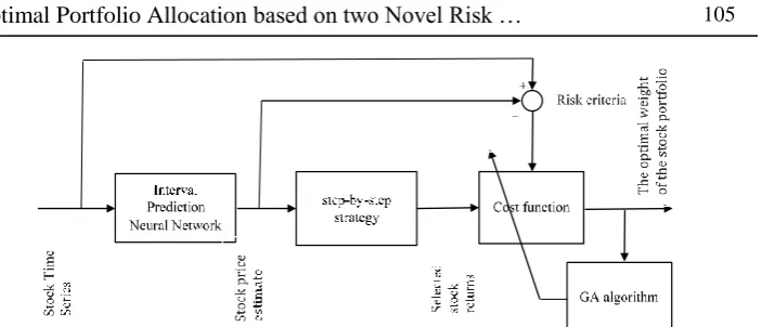
This function is based on the difference in stock weight over two consecutive periods. If the weight of the i-th share decreases in the next period, this difference will be negative and 𝑡𝑟 = 𝑠𝑝. Also, if the weight of i-th share in i-the next period increases, i-this difference will be positive and 𝑡𝑟 = 𝑏𝑝. Thus, both buy and sale penalties for each share will be easily applied. Afterward, the mentioned optimization problem will be solved by a global search algorithm such as Genetics algorithm. It is not a wise decision to incorporate all the stock in the portfolio in each stage of optimization. Because the optimization problem solving process will be too time consuming. A strategy called step-by-step is used to overcome this problem. This strategy states that we only buy a stock that has a higher price growth than a predetermined threshold and only sell shares that lower price drop than a specified threshold percentage (this is the desired limit, which is assumed to be 5% here). Therefore, if the stock price in the portfolio did not change much (whether ascending or descending), it will not take part in the optimization. This strategy is also closer to human thinking and it also causes all the stock in the portfolio not to enter the algorithm at each optimization step and so the time duration of the optimization problem will be greatly reduced. This strategy is expressed in (19):
{𝑖𝑓
‖𝑥̂𝑡+𝑛−𝑥𝑡‖
𝑥𝑡 ≫ 0.05 → 𝑥𝑡 𝑠𝑒𝑙𝑒𝑐𝑡𝑒𝑑 𝑓𝑜𝑟 𝑜𝑝𝑡𝑖𝑚𝑖𝑧𝑎𝑡𝑖𝑜𝑛
𝑜𝑡ℎ𝑒𝑟 → 𝑥𝑡 𝑛𝑜𝑡 𝑠𝑒𝑙𝑒𝑐𝑡𝑒𝑑 𝑓𝑜𝑟 𝑜𝑝𝑡𝑖𝑚𝑖𝑧𝑎𝑡𝑖𝑜𝑛
(19)
Fig. 2. Diagram of the proposed method for determining the stock optimal portfolio
4. Simulation
In this section, the proposed algorithm for predicting stock prices and modeling the capital allocation problem with the two risk measures presented in Section 3, is simulated for the data of 18 shares of the Tehran Stock Exchange during the period from 12/2/2012 to 13/4/2016. The stock list selected is provided in Table 1.
Table 1. Selected stocks to be present in the portfolio with number indices
GOGEL (1) VOTSOUM (2) MADARAN (3) GHAPINO (4) KASEFA (5) KAHIFEH (6)
WASINA (7) KAMA (8) JAM (9) KHARIJK (10) GHADASHT (11) PARSAN (12)
ZAHDER (13) KHOSAZ (14) SAHASHAH (15) GHASALM (16) KHORRAM (17) WAGHADIR (18)
The first step is the training of the differential MLP neural network to predict the price of the 18 shares. Since we want to change the allocation of capital every 5 days, the forecast horizon is considered to be 5 days. In Table 2, the mean variance of the normalized estimation error (mse) of the prediction of price for each of the 18 stocks for the next 5 days has been presented.
Table 2. Mean variance of normalized estimation error (mse) of the price prediction for next 5 days
Stock No. 1 2 3 4 5 6 7 8 9
mse 0.1396 0.0003 0.0098 0.0060 0.0716 0.0870 0.0018 0.1252 0.1308
Stock No. 10 11 12 13 14 15 16 17 18
The predictions made by the differential neural network for only two shares of KHOOSAZ and WAGHADIR as an example of the stock portfolio available, are shown in Fig. 3. The normalized estimation error of these two shares is also shown in Fig. 4. Neural networks trained to predict share prices in the next 5 days have been used and the above variances are used as a risk measure.
Fig. 3. Real stock price and stock price data predicted by the MLP differential neural network
Fig. 4. Normalized estimation error in two sample shares
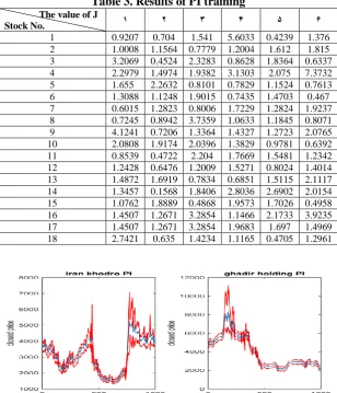
The second proposed criterion for the risk is the PI's width. In this regard, for each of the 18 shares, separately, another PI-based neural network with two hidden layers, by the training LUBE algorithm and for the 6 different neuron modes and for each case, the neural network training process is performed 3 times. In Table 3, the average 𝐽 = 𝑃𝐼𝐶𝑃
𝑃𝐼𝑁𝑅𝑊 of trained neural
6 Neuron modes are as follows:
(1) 3 neurons in the first layer and 1 neuron in the second layer (2) 3 neurons in the first layer and 2 neurons in the second layer (3) 5 neurons in the first layer and 1 neuron in the second layer (4) 5 neurons in the first layer and 2 neurons in the second layer (5) 7 neurons in the first layer and 1 neuron in the second layer (6) 7 neurons in the first layer and 2 neurons in the second layer
The PIs of the two KHOOSAZ and WAGHADIR shares are listed as examples in Fig. 5.
Table 3. Results of PI training
6 5 4 3 2 1
The value of J
Stock No. 1.376 0.4239 5.6033 1.541 0.704 0.9207 1 1.815 1.612 1.2004 0.7779 1.1564 1.0008 2 0.6337 1.8364 0.8628 2.3283 0.4524 3.2069 3 7.3732 2.075 3.1303 1.9382 1.4974 2.2979 4 0.7613 1.1524 0.7829 0.8101 2.2632 1.655 5 0.467 1.4703 0.7435 1.9015 1.1248 1.3088 6 1.9237 1.2824 1.7229 0.8006 1.2823 0.6015 7 0.8071 1.1845 1.0633 3.7359 0.8942 0.7245 8 2.0765 1.2723 1.4327 1.3364 0.7206 4.1241 9 0.6392 0.9781 1.3829 2.0396 1.9174 2.0808 10 1.2342 1.5481 1.7669 2.204 0.4722 0.8539 11 1.4014 0.8024 1.5271 1.2009 0.6476 1.2428 12 2.1117 1.5115 0.6851 0.7834 1.6919 1.4872 13 2.0154 2.6902 2.8036 1.8406 0.1568 1.3457 14 0.4958 1.7026 1.9573 0.4868 1.8889 1.0762 15 3.9235 2.1733 1.1466 3.2854 1.2671 1.4507 16 1.4969 1.697 1.9683 3.2854 1.2671 1.4507 17 1.2961 0.4705 1.1165 1.4234 0.635 2.7421 18
In recent years, the CVaR as the mean of the tail of the probability density (risk greater than VaR) has attracted a lot of attention. The CVaR as a risk criterion has shown better characteristics than VaR. This risk criterion measures the expected risk when it is greater than the specified percentile (VaR), indicating that, if the conditions are unfavorable, how much risk would it have? In other words, CVaR indicates that if changes in the stock portfolio value are likely to be (1 − 𝛼) in the tail section of the probability density curve, then how much is the risk during a n-day period [42]. For comparing the efficiency of the proposed two risk measures, the criterion of CVaR is used in the following equation [42]:
𝐶𝑉𝑎𝑅𝛽(𝑥) = (1 − 𝛽)−1∫ 𝑓(𝑥, 𝑦)𝑝(𝑦)𝑑𝑦 𝑎
𝑓(𝑥,𝑦)≥𝑉𝑎𝑅𝛽(𝑥) . (20)
Afterward, the problem of 5-day period capital allocation is solved for three modes using the genetic algorithm. At this stage, as outlined in Section 3, the step-by-step strategy is applied. Thus, the low speed of the genetic algorithm is not too troublesome, and we can still take advantage of the global search capability. At each stage, only stocks with more than 5% price change are entering the optimization process. Of course, this measurement of price change is obtained using the subtraction of price predicted by the neural network for each share for the next 5 days and the current price. Therefore, the optimization problem has been solved and the normalized returns are calculated in each step. This return is as follows:
𝑅𝑡𝑜𝑡𝑎𝑙(𝑘) = (1 + 𝑟𝑟1)(1 + 𝑟𝑟2) … (1 + 𝑟𝑟𝑘) − 1. (21)
Where 𝑟𝑟𝑗 is the real return of the j step compared to the previous step and
is derived from the sum of the individual stock returns in the portfolio. It should be noted that the following equation was used to calculate the return on each share:
𝑟𝑟𝑖𝑗= [𝑤𝑖𝑗𝑟𝑖𝑗− [𝑤𝑖𝑗− 𝑤𝑖(𝑗−1)]. 𝑡𝑟(𝑤𝑖𝑗− 𝑤𝑖(𝑗−1))]. (22)
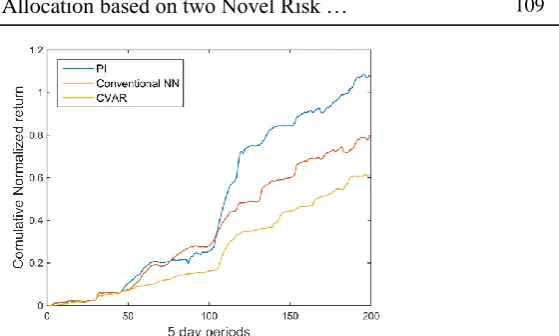
Fig. 6. Normalized returns with 5-day periods for portfolio modification with three criteria of error variance, PI width and CVaR
It should be noted that all three methods have positive and upward returns over time. However, in all stages, the state of the PI-based risk has higher return. This comes from the fact that in a PI-based risk state, a fixed value is not assigned to the risk. In the first case, noise and uncertainty are assumed to be uniformly distributed at all times, while this is not the case in practice and the uncertainties in stock price data are affected by varying factors over time. In either case, the result of CVaR was better.
Table 4. The weight of different stocks in the portfolio for three different risk states
Stock No.
Stock weight in risk mode with estimated error variance
Stock weight in risk mode with PI width Stock Weight in
CVaR Risk 1 0.0224 0.0169 0 2 0 0 0.0406 3 0.1333 0.1534 0.036 4 0.0266 0.02 0.0379 5 0.0128 0.0096 0.0319 6 0.0685 0.0018 0.4249 7 0.0158 0.0258 0.0359 8 0.0044 0.154 0.038 9 0 0 0.0363 10 0 0 0.0364 11 0.3613 0.1272 0.0373 12 0.0011 0.0013 0.0378 13 0.04 0.0301 0.0394 14 0.0653 0.0491 0.0298 15 0 0 0.0384 16 0 0 0.0296 17 0.0059 0.0026 0.0382 18 0.2424 0.5467 0.0323 Conclusion
In this paper, MLP neural networks were used to predict stock prices. These predictions were considered as the expected returns of different stocks. The risk of these predictions should also be taken into account to make the allocation process more realistic. The proposed approach utilized the uncertainty of neural network in the prediction of output. Once the error variance of neural network training phase estimation was used as a constant risk value, afterward the interval prediction neural network using PI width for the test data was applied as a time-varying risk. Then, a cost function was proposed for simultaneous consideration of the proposed risk and expected returns, and the problem of optimal allocation of capital to different stocks was modeled as a single-objective optimization problem.
References
1. Ou, J. A., & Penman, S. H. Financial statement analysis and the prediction of stock returns. Journal of accounting and economics, 11(1989), 295-329.
2. Patra, A., Das, S., Mishra, S. N., & Senapati, M. R. An adaptive local linear optimized radial basis functional neural network model for financial time series prediction. Neural Computing and Applications, 28(2017), 101-110.
3. Zhang, L., Wang, F., Xu, B., Chi, W., Wang, Q., & Sun, T. Prediction of stock prices based on LM-BP neural network and the estimation of overfitting point by RDCI. Neural Computing and Applications, (2017), 1-20.
4. Adhikari, R., & Agrawal, R. K. A combination of artificial neural network and random walk models for financial time series forecasting. Neural Computing and Applications, 24, (2014), 1441-1449. 5. Armano, G., Murru, A., & Roli, F. Stock market prediction by a mixture of genetic-neural experts. International Journal of Pattern Recognition and
Artificial Intelligence, 16(2002), 501-526.
6. Bishop, C. M. Neural networks for pattern recognition. Oxford university press. 1995.
7. Wu, J. Hybrid Optimization Algorithm to Combine Neural Network for Rainfall-Runoff Modeling. International Journal of Computational
Intelligence and Applications, 15(2016), 1650015.
8. Park, D. C., Woo, D. M., Kim, C. S., & Min, S. Y. Clustering of 3D line segments using centroid neural network for building detection. Journal of
Circuits, Systems, and Computers, 23(2014), 1450071.
9. HUANG, Y. P., WEN, S. Y., XIANG, W. C., & JIN, Y. S. PID Parameters Self-tuning Based on Genetic Algorithm and Neural Network. Artificial Intelligence, 10(2016), 9789813206823_0003.
10. Liu, W. H... Forecasting the semiconductor industry cycles by bootstrap prediction intervals. Applied Economics, 39(2007), 1731-1742.
11. Khosravi, A., Nahavandi, S., & Creighton, D. Construction of optimal prediction intervals for load forecasting problems. IEEE Transactions on
Power Systems, 25(2010), 1496-1503.
12. Zhao, J. H., Dong, Z. Y., Xu, Z., & Wong, K. P. A statistical approach for interval forecasting of the electricity price. IEEE Transactions on Power
Systems, 23(2008), 267-276.
13. Pierce, S. G., Worden, K., & Bezazi, A. Uncertainty analysis of a neural network used for fatigue lifetime, prediction.Mechanical Systems and
Signal Processing, 22(2008), 1395-1411.
14. Benoit, D. F., & Van den Poel, D. Benefits of quantile regression for the analysis of customer lifetime value in a contractual setting: An application in financial services. Expert Systems with
Applications, 36(2009), 10475-10484.
15. Shrestha, D. L., & Solomatine, D. P... Machine learning approaches for estimation of prediction interval for the model output. Neural
16. Van Hinsbergen, C. I., Van Lint, J. W. C., & Van Zuylen, H. J. Bayesian committee of neural networks to predict travel times with confidence intervals. Transportation Research Part C: Emerging
Technologies, 17(2009), 498-509.
17. Khosravi, A., Mazloumi, E., Nahavandi, S., Creighton, D., & Van Lint, J. W. C. Prediction intervals to account for uncertainties in travel time prediction. IEEE Transactions on Intelligent Transportation Systems, 12 (2011), 537-547.
18. Khosravi, A., Mazloumi, E., Nahavandi, S., Creighton, D., & Van Lint, J. W. C. A genetic algorithm-based method for improving quality of travel time prediction intervals.Transportation Research Part C: Emerging
Technologies, 19 (2011), 1364-1376.
19. Khosravi, A., Nahavandi, S., & Creighton, D... A prediction interval-based approach to determine optimal structures of neural network metamodels. Expert systems with applications, 37(2010), 2377-2387. 20. Chryssolouris, G., Lee, M., & Ramsey, A. Confidence interval prediction for neural network models. IEEE Transactions on neural
networks, 7(1996), 229-232.
21. Hwang, J. G., & Ding, A. A. Prediction intervals for artificial neural networks. Journal of the American Statistical Association, 92 (1997), 748-757.
22. Wild, C. J., & Seber, G. A. F. Nonlinear regression. 1989.
23. De VlEAUX, R. D., Schumi, J., Schweinsberg, J., & Ungar, L. H. Prediction intervals for neural networks via nonlinear regression. Technometrics, 40(1998), 273-282.
24. Ho, S. L., Xie, M., Tang, L. C., Xu, K., & Goh, T. N. Neural network modeling with confidence bounds: a case study on the solder paste deposition process. IEEE Transactions on Electronics Packaging
Manufacturing, 24(2001), 323-332.
25. Lu, T., & Viljanen, M. Prediction of indoor temperature and relative humidity using neural network models: model comparison. Neural
Computing and Applications, 18(2009), 345.
26. AKhosravi, A., Nahavandi, S., & Creighton, D. Improving prediction interval quality: A genetic algorithm-based method applied to neural networks. InInternational Conference on Neural Information Processing,
2009 (pp. 141-149). Springer, Berlin, Heidelberg.
27. MacKay, D. J. The evidence framework applied to classification networks. Neural computation, 4(1992), 720-736.
28. Heskes, T. Practical confidence and prediction intervals. In Advances
in neural information processing systems, (1997), (pp. 176-182).
29. Dybowski, R., & Roberts, S. J. Confidence intervals and prediction intervals for feed-forward neural networks.Clinical Applications of
Artificial Neural Networks, 2001, 298-326.
30. Oleng, N. O., Gribok, A., & Reifman, J. Error bounds for data-driven models of dynamical systems. Computers in biology and
31. Aouni, B. Multi-attribute portfolio selection: New perspectives. INFOR: Information Systems and Operational
Research, 47(2009), 1-4.
32. Mainik, G., Mitov, G., & Rüschendorf, L. Portfolio optimization for heavy-tailed assets: Extreme Risk Index vs. Markowitz. Journal of
Empirical Finance, 32(2009), 115-134.
33. Markowitz, H. Portfolio selection. The journal of finance, 7(1952, 77-91.
34. Rockafellar, R. T., & Uryasev, S. Optimization of conditional value-at-risk. Journal of risk, 2(2000), 21-42.
35. Quan, H., Srinivasan, D., & Khosravi, A. Construction of neural network-based prediction intervals using particle swarm optimization.
In Neural Networks (IJCNN), The 2012 International Joint Conference on,
2000, (2012). (pp. 1-7). IEEE.
36. Khosravi, A., Nahavandi, S., Creighton, D., & Atiya, A. F. Lower upper bound estimation method for construction of neural network-based prediction intervals. IEEE Transactions on Neural Networks, 22(2011), 337-346.
37. Chow, T. W. S., & Leung, C. T. Neural network based short-term load forecasting using weather compensation. IEEE Transactions on Power
Systems, 11(1996), 1736-1742.
38. Pavelka, A., & Procházka, A. Algorithms for initialization of neural network weights. In In Proceedings of the 12th Annual Conference,
MATLAB, (2004), (pp. 453-459).
39. Eberhart, R., & Kennedy, JA new optimizer using particle swarm theory. In Micro Machine and Human Science, 1995. MHS’95. Proceedings of the Sixth International Symposium on, (1995) (pp. 39-43). IEEE.
40. [Huang, N. E., Wu, M. L., Qu, W., Long, S. R., & Shen, S. S. Applications of Hilbert–Huang transform to non‐stationary financial time series analysis. Applied stochastic models in business and
industry, 19(2003), 245-268.
41. Clements, M. P., & Hendry, D. F. Forecasting non-stationary
economic time series. Mit Press. 2001.
42. Quan, H., Srinivasan, D., & Khosravi, a Short-term load and wind power forecasting using neural network-based prediction intervals. IEEE