Smart Energy Systems: using IoT Embedded Architectures for Implementing a Computationally Efficient Synchrophasor Estimator

(1)

Smart Energy Systems:

using IoT Embedded Architectures for Implementing a

Computationally Efficient Synchrophasor Estimator

Author:

Pietro TOSATO

Advisors: Dr. Davide BRUNELLI Dr. David MACII

A thesis submitted in fulfillment of the requirements for the PhD degree

at the

Doctoral School in Materials, Mechatronics and Systems Engineering Department of Industrial Engineering

(2)

(3)

(4)

Acknowledgements

Few but sincere words to whom help and support me during this journey of (more than) three years. My heartfelt gratitude and esteem to Davide Brunelli and David Macii, two great advisors and teachers during this period: thanks for the huge support during this adventure!

Thanks to my friends and colleagues in Trento, the ones in laboratory and all whom I had the chance to talk with and learn something new, in particular to Maurizio and Matteo. A special mention goes to the friendly colleagues I met during my stay in Belfast, starting from David, John, Paul and Judith.

Thanks to the dear Valentina, Elena, Andrea, Stefano, Luca and Sofia for distracting me from this cruel world.

Thanks to Giulia who supports my period abroad from the distance, and keep supporting me, ironically still from some hundreds kilometers: I feel very lucky to have someone like you trusting, supporting and bearing me, I love you.

Last, but not least, a sincere thank to my parents and my family for incessantly bearing me.

(5)

(6)

List of Figures

1.1 Overall architecture of the prototype. Dashed arrows indicate enable and feedback signals (EN and FB) while continued line arrows are power flows. . . 11 1.2 P-V characteristics of considered mini PV arrays at 500 lux (a) and 1

klux (b) . . . 12 1.3 In (a) the data collected from the laboratory prototype as indoor

ir-radiance near window and relative power havested by the system, while in (b) the on-the-field prototype location. (from [32] with per-missions) . . . 13 1.4 Prediction of the feasible energy neutral operations, based on the

measurements on the prototype, with respect to the fixed sensing periods (45 minutes or 1 hour) and the hours of light per day. . . 14 1.5 Sensitivity of low power RF based wake-up receivers vs. power

con-sumption. Different symbols refers to different modulation schemes, as in the legend. (from [33] with permissions) . . . 17 1.6 Overall architecture and picture of the prototype. Dashed arrows

in-dicate trigger (TRIG) and signaling (FB) while continued line arrows are power flows. (from [38] with permissions) . . . 18 1.7 Static Power-Voltage diagram of a PMFC (from [44] with permissions) 19 1.8 Power consumption measurement of the remote sensor node with

radio-trigger. The measurement starts at the trigger (A), then the node boot (B) and finally transmit the measure (C). (from [38] with permissions) . . . 21 1.9 In (a) the signal demodulator circuit: two branch on the voltage

(11)

1.10 Scope acquisitions of the comparator signals in (a) the two input sig-nals that come from two branches of the voltage multiplier, and in (b) the output of the comparotor with respect to the input signal of the PLC wake-up system. . . 26 1.11 Picture of the prototype produced with the main PLM in (a) and in a

prototype version in (b). . . 27 1.12 Example of a street lighting network as it was simulated. . . 28 1.13 Equivalent circuits for simulating the cable transmission line, an

elec-tronic ballast and the coupling section of the modem. . . 31 1.14 Schematic of the model used to validate the parameters of the cable. 32 1.15 Schematic of a realistic street lighting network. (from [71] with

per-missions) . . . 33 1.16 Example of a street lighting network as it was simulated with the

addition of the wake-up receivers. . . 34

2.1 A couple of example waveforms, with a phase difference of 90 de-grees and the respective phasor representation (with the same color). 44 2.2 Difference between the coherent and not coherent operation of a

PMU. These effects can be caused by both sampling frequency prob-lems and frequency offsetδ. The red dots indicate the time instant when the phasor is computed and, in the plots on the bottom, the result measured phase is shown. . . 45

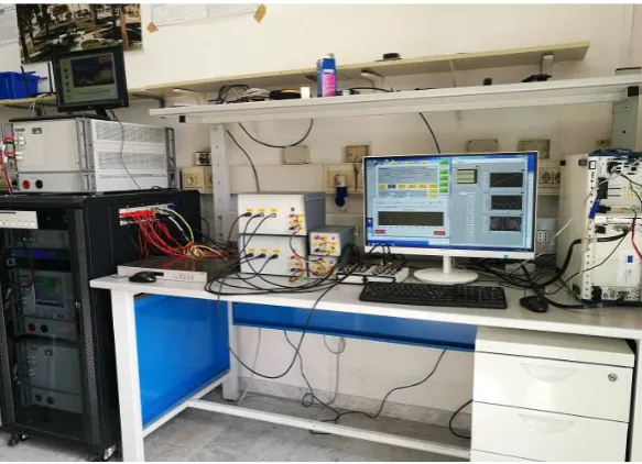
3.1 Picture of the testbed. . . 59 3.2 Block Diagram of the testbed. (from [124] with permissions) . . . . 62 3.3 Estimated PSDΦG(f)of the noise introduced by the Fluke 6135A/PMUCAL.

. . . 66 3.4 Estimated PSDΦT(f)of the noise introduced by transducer.

Respec-tively, (a) is the LEM CV3-1000 and (b) the ABB TV2-380/100. . . 67 3.5 Estimated PSDΦD(f)of the noise introduced by the data acquisition

module (NI PXIe-6124). . . 68 3.6 Estimated PSDΦS(f)of the noise introduced by the Synchronization

module (NI PXI-6683H). . . 69

4.1 Phasor estimation via demodulation and filtering approach, as in the Annex of the standard C37.118.1 [103]. . . 77 4.2 Flow chart of the TLTFT estimation algorithm. . . 83 4.3 Experimental results (phase and frequency errors) using a chirp

(12)

5.1 Picture of a BeagleBone Black board. . . 99 5.2 AM3358 functional diagram. From http://www.ti.com/product/

AM3358 . . . 100 5.3 Processing time comparison between the TLTFT and the algorithm

in [163] for different number of samplesN andC = 7. (from [184] with permissions) . . . 102 5.4 Maximum processing time of TLTFT algorithm on the BeagleBone

Black. The curves are made changing the sampling frequency and observation interval lengthC . . . 103 5.5 Maximum SNR values for which the RFE is smaller than 1/2 of the

stricter limits of the standard τRFE as function of the sampling

fre-quency, for different observation interval lengthsC. . . 104 5.6 Example design of possible trade-offs between maximum processing

(from Fig. 5.4) time and maximum SNR (from equation (5.1)). The ar-rows refer to the resulting SNR levels for a given sampling frequency of 8 kHz. . . 105 5.7 Architecture of the Acquisition and synchronization blocks as

im-plemented in the OpenPMU project. (from [170] with permissions) . . . 107 5.8 Model of the classic Servo Clock. (from [192] with permissions) . . . 108 5.9 Stability region of the servo clock as a function of the PI coefficients. 110 5.10 Architecture of the SC implemented on the PRU of the BBB. (from

[192] with permissions). . . 111 5.11 Model of the servo clock as implemented on the BBB. (from [192]

with permissions) . . . 111 5.12 Surface plot of the variances given by equations (5.15) on the left,

and (5.16) on the right, as function of the parametersKPandKI. . . . 114

5.13 Experimental values of standard deviation of the synchronization er-rors for different values of the controller parametersKP andKI. . . . 116

5.14 Allan deviation plots obtained from the PPS signals for different con-trol laws as in the legend. For comparison, also the Allan deviation of the free-running clock is shown. . . 117 5.15 Histograms of the PPS period fluctuations generated by the SC,

us-ing different controllers, i.e. in (a) the the dead-beat, in (b) the quasi-optimal controller withKP = 1 andKI = 0.05 and in (c) the

unity-gain controller. All the plot are normalized on the percent probability. 118

(13)

(14)

List of Tables

1.1 Laboratory measurement of power consumptions and efficiency of the components of the pollution monitoring node. . . 14 1.2 Laboratory measurement of power and current consumptions of the

components of the node. . . 22 1.3 _{Simulated peak-to-peak voltage amplitude of a 10 VPP FSK signal in}

different points of a street lighting network. (from [71] with permis-sions) . . . 32 1.4 _{Simulated peak-to-peak voltage amplitude of a 10 VPP FSK signal in}

different points of a street lighting network, with the branches as in Figure 1.12. (from [71] with permissions) . . . 34 1.5 Minimum energy associated to the wake-up operation of a node

ad-dressed with a defined number of retransmissions of the wake-up message (hops). . . 35

2.1 Test conditions for both P and M class PMU, for the steady-state compliance reported in IEEE Std. C37.118.1 [103] considering the Amendment [105]. . . 50 2.2 TVE, FE and RFE limits for both P and M class PMU, for the

steady-state compliance tests of the IEEE Std. C37.118.1 [103] considering the Amendment [105]. The symbol (*) refers to the most stringent limit in the Standard, which depends on the reporting rate, while the “-” means that either the class does not require the specific per-formance or that the perper-formance limit has been suspended. . . 51 2.3 Test conditions for both P and M class PMU, for the AM and PM test

signals for compliance reported in IEEE Std. C37.118.1 [103] consid-ering the Amendment [105]. ka andkpare defined in equation (2.5).

(15)

2.4 Compliance limits for both P and M class PMU, for the dynamic compliance tests (AM and PM modulation and frequency ramp) of the IEEE Std. C37.118.1 [103], considering the Amendment [105]. The symbol (*) refers to the most stringent limit in the standard, which depends on the reporting rate.. . . 53 2.5 Test conditions for both P and M class PMU, for the step test of

the IEEE Std. C37.118.1 [103], considering the Amendment [105]. The response time requirement is different for phasor, frequency and ROCOF measurements: here is reported only the phasor response time, which is the strictest. . . 54

3.1 Fluke 6135/PMUCAL specifications for the test under C37.118.1a [105]. 59 3.2 Measured value and standard uncertainties of the parameters of the

model. . . 70 3.3 Absolute values of the difference between the maximum TVe, FE and

RFE measured using pure sinewaves of given frequency and the cor-responding Monte Carlo simulation with a comparable noise floor (SNR=60 dB). . . 72 3.4 Absolute values of the difference between the maximum TVe, FE

and RFE measured using pure sinewaves of given frequency and the corresponding Monte Carlo simulation with a negligible noise floor (SNR=120 dB). . . 73 3.5 Maximum TVE, FE and RFE values obtained in different testing

con-ditions for both simulated environment and testbed. The reported results belong to different AUTs (i.e. IpD2FT, IpDFT and TWLS), with an observation intervalC=4 nominal power line cycles and report-ing rate equal to 50 Hz. . . 74

4.1 Maximum TVE, FE and RFE values obtained in simulation for some Class P tests reported in the IEEE Standards C37.118.1-2011 and C37.118.1a-2014 when observation lengths ofC={2, 3, 4}cycles are considered andfs=8 kHz. The IEEE C37.118.1a-2014 limits when the reporting

rate is 50 fps are shown as well. . . 91 4.2 Maximum TVE, FE and RFE values obtained in simulation for some

Class M tests reported in the IEEE Standards C37.118.1-2011 and C37.118.1a-2014 when observation intervals ofC = {5, 6, 7}cycles are considered and fs = 8 kHz. The IEEE C37.118.1a-2014 limits

(16)

4.3 Maximum TVE, FE and RFE values obtained on the testbed for some Class P tests reported in the IEEE Standards C37.118.1-2011 and C37.118.1a-2014 when observation lengths ofC= {2, 3, 4}cycles are considered and fs =8 kHz. The IEEE C37.118.1a-2014 limits when the reporting

rate is 50 fps are shown as well. . . 93 4.4 Maximum TVE, FE and RFE values obtained on the testbed for some

Class M tests reported in the IEEE Standards C37.118.1-2011 and C37.118.1a-2014 when observation intervals of C = {5, 6, 7}cycles are considered and fs = 8 kHz. The IEEE C37.118.1a-2014 limits

when the reporting rate is 50 fps are shown as well. . . 94

5.1 An hardware comparison of some recent PMU implementations. . . 97 5.2 Performance of the Meinberg M600 equipped with standard quality

OCXO [195]. . . 115

B.1 Common cosine windows and relative parameters . . . 128

(17)

(18)

List of Abbreviations

ADC Analog toDigitalConverter

BBB BeagleBoneBlack

DER DistributedEnergyResource

DFT DiscreteFourierTransform

DSP DigitalSignalProcessor

DSO DistributionSystemOperator

FE FrequencyError

FIR FiniteImpulseResponse

GPS GlobalPositioningSystem

IoT InternetofThings

IRIG-B Inter-RangeInstrumentationGroup - formatB

PDC PhasorDataConcentrator

PMU PhasorMeasurementUnit

PPS PulseperSecond

PRU ProgrammableReal-timeUnit

PSD PowerSpectralDensity

ROCOF RateOfChangeOfFrequency

RFE Rate of change ofFrequencyError

RMS RootMeanSquared

SC ServoClock

SFDR Spurious-FreeDynamicRange

SINAD Signal-to-NoiseandDistortion

SNR Signal-to-NoiseRatio

THD TotalHarmonicDistortion

TVE TotalVectorError

UTC CoordinatedUniversalTime

WAMS Wide-AreaManagementSystem

WLS WeightedLeastSquares

(19)

(20)

Introduction

Motivations of the thesis

Energy efficiency is a key challenge to build a sustainable society. It can be declined in variety of ways: for instance, from the reduction of the environmental impact of appliances manufacturing, to the implementation of low-energy communication networks, or the management of the existing infrastructures in a smarter way. The actual direction is the integration of different energy systems with a common man-agement scheme with the aim of harmonizing and integrating different energy sys-tems.

In this context, smart cities already envision the use of information communica-tion technologies (ICT) to smartify objects and services, connecting people and ma-chines. An important enabling technology for smart cities is certainly the Internet of Things (IoT).

(21)

bring in energy production and the hazard they may represent if not properly man-aged (e.g. violation of operational constraints). ADN implementation relies on the deployment of high-performance real-time monitoring and control systems.

It is well accepted that the phasor measurement units (PMU) are one of the most promising instruments to overcome many problems in ADN management, as they support a number of applications, such as grid state estimation, topology detec-tion, volt-var optimization and reverse power flow management. However, classic PMUs are conceived to measure synchrophasor in transmission systems, while the distribution ones have very different characteristics and, in general, different needs. Therefore, tailoring the characteristics of the new-generation PMUs to the needs of the ADNs is currently very important. This new kind of PMU must address few important design challenges:

1. improved angle measurement capabilities, to cope with the smaller angle dif-ferences that distribution grids exhibit;

2. low cost, to promote an extensive deployment in the grid.

These two requirements are clearly in opposition.

In this dissertation, a low-cost PMU design approach, partially influenced by IoT ideas, is presented.

In particular, this thesis is organized as follow.

Organization of the thesis

(22)

network application. A section on the power grid needs and the future smart grid concludes the chapter.

In Chapter2, the basics of synchrophasor measurement are introduced. The defini-tion, nomenclature and models for synchrophasor measurements are given. Then, the standards for PMU compliance testing are presented.

To better understand how a PMU works and what the main uncertainties contri-butions affecting the synchrophasor measurement are, a PMU testbed is described in Chapter3. The characterization of such a system based on a noise propagation model helps the developer to understand the impact of different uncertainty con-tributions.

Chapter 4 deals with a novel algorithm conceived for a low-cost PMU based on

performance-constrained embedded platforms. The analysis of the performance of the algorithm is split between Chapter4, where the metrological performance are analyzed, and Chapter 5, where the trade-offs needed to ensure real-time perfor-mances are discussed.

In particular, after a description of a low-cost PMU implementation, the evaluation of timing performance of the proposed algorithm is presented in Chapter5, along with relevant details on synchronization and syntonization for data acquisition. A servo clock for PMU synchronization is implemented and characterized for this purpose.

Chapter 6 concludes the thesis with a summary, some final remarks and future

work.

Contributions of the thesis

This dissertation contributes to the implementation of modern smart energy sys-tem, inspired by state of the art IoT solutions to reduce power consumption while improving services and operations. This is declined in a couple of different ways: energy efficient IoT solutions and a low-cost yet effective implementation of PMU to modernize ADNs.

(23)

idea comes from the wireless counterpart, i.e. wake-up radios, which are presented in this dissertation as well.

A low-cost PMU implementation A PMU running on a low-cost platform is en-visioned. To this goal, an algorithm for synchrophasor, fundamental frequency, and rate of change of frequency estimation is developed for processing platforms with limited computational resources .

The proposed solution harnesses the main advantages of two state-of-the-art algo-rithms, namely the Interpolated Discrete Fourier Transform (IpDFT) and the Taylor Fourier Transform (TFT). A new algorithm is proposed and implemented in a com-putationally efficient manner to reduce processing time as much as possible. To this aim, the number of harmonics accounted in the model is changed adaptively to minimize the computational burden while meeting the main requirements speci-fied in the IEEE standards C37.118.1 and the Amendment C37.118.1a. The resulting processing time of the algorithm is compliant with the mandatory reporting peri-ods of M class or P class PMU. Estimation accuracy has been evaluated not only through simulations but also experimentally.

A servo-clock (SC) for PMUs is also proposed. The SC relies on a classic propor-tional integral controller, which has been properly tuned to minimize the steady-state short-term time synchronization uncertainty. The SC has been implemented and tested on a PMU prototype developed within the OpenPMU project. The distinctive feature of the proposed solution is its ability to track an input Pulse-Per-Second reference with good stability and with no need for specific on-board synchronization circuitry. Indeed, the SC implementation relies only on only one co-processor of the chosen platform.

(24)

CHAPTER 1

Energy Efficiency in Smart Cities

In this chapter, a broad vision of energy efficiency enablers for smart cities is given. The vari-ous and rather heterogenevari-ous sections deal with different examples of low-power technologies. The discussion, however, follows a specific plot, describing technology and relative applica-tions in different fields. In particular, the following secapplica-tions present IoT technologies with few design examples, including smart lighting. Finally, the power system research trends are introduced.

1.1

Introduction

While the world population breaches the 7 billions threshold, mostly agglomerated in metropolitan areas, several problems still require smart solutions, for instance in transportation, environment and quality of life, among others.

European Union, is active and sensitive in this context, promoting plans and action to reduce energy consumption and all the wastes which, in general, cause high pollution levels. Horizon 2020is one of the biggest research funding program ever, which“help to achieve smart, sustainable and inclusive growth”. Till 2020, European Union agenda is clear in fixing three targets regarding energy:(i)−20 % greenhouse gas (GHG) emission (with respect to 1990),(ii)20 % share of energy coming from renewable sources and(iii)+20 % in energy efficiency [1]. These goals, even if seem ambitious, are likely to be achieved. For 2030, EU has reinforced this message with new targets, like the 27 % share of energy that comes from renewable sources [2].

(25)

processes to networking, energy efficiency is always a need, as energy is becoming more and more valuable, even if people tend to forget it. After a long period of wastes, in the era of smart cities, the energy systems also have to become smarter, to solve, at least partially, some environmental problems.

The smart city buzzword is around from few years now, and many definitions were formulated, all of them relying on the same concept of making better use of re-sources increasing quality of services by exploiting Information Communication Technologies (ICT) [3]. Because of its broad scope, smart city embrace many re-search fields, not only ICT-related. This synergy often permits to obtain valuable results from many perspectives. In fact, the concept of smart energy systems, also relies on the joint effort coming from different domains (e.g. thermal, electrical and gas grids combined) to create a sustainable and affordable energy future [4]. Both academia and industry are now focusing on developing strategies for imple-menting the smart city. For instance, IEEE has promoted the Smart City Commu-nity, to raise awareness around topics like smart living, sustainable energy man-agement and smart mobility, and the Smart Cities Initiative to facilitate and boost collaborative work between different societies like Communication Society, Power & Energy Society, and others. Large companies like IBM, CISCO and Intel are in-volved in various projects for smart city creation.

Some smart cities around the world are already recognized, and already have im-plemented smart systems to handle (i) power grid, (ii) buildings and (iii) light-ing [5], [6]. On these three domains in particular, the aim is not only the improve-ment of the quality of the system, making it smarter, but also facing major problems like environmental pollution, the scarcity of natural resources or climate changes. The reduction of greenhouse gases is also a great challenge for the XXI century, addressable only with enhanced smart energy systems.

Energizing the city Including the current concept of smart grid into the big smart city container is not fully rightful. However, electricity transmission and distribu-tion have a clear impact on everyday life, which is expected to be even more im-portant in the future due to the penetration of electrical mobility. More in general, smart city solutions must be energy efficient and tackle the associated challenges. It would be shortsighted to exclude the grid energy efficiency from the broad vision of a smart city. Currently, citizens have also become more aware about energy use and waste, especially as far as electricity is concerned. The border sometimes is also not clearly visible even in literature contributions: the termsmart energy system

in fact is used as a synonym ofsmart gridby some authors [4].

(26)

of many researchers and are currently envisioned as a key for future electricity sys-tems (in addition to energy storage and demand response) [7].

Of course, energy efficiency should be primarily achieved by reducing the power consumptions of buildings. In fact, they consume the biggest share of primary energy, more than any other sector (for instance, approximately 40 % in heating, air conditioning and lighting) [8].

To cope with this and many other energy challenges, ICT can provide a great help.

Networking the city Internet offers sophisticated and ubiquitous networking for smart city services. The buzzword today isInternet of Things, the communication paradigm that envision objects of everyday life equipped with connectivity and the possibility to communicate to each other and to the user, becoming part of the In-ternet [9]. In turn, Internet will become even more pervasive than it is today. This is a key to“smartify”the existent smart city component systems or building the new generation ones, especially buildings, energy grids and lighting systems. As pre-viously stated, energy efficiency is the challenge to address in order to implement successful services without impact on the environment. Of course, IoT devices also have to be efficient and consume as less power as possible, avoiding energy over-heads and achieving a seamless integration of the ICT infrastructure [10].

1.2

The role of IoT

Human being is building an intricate and huge network, pervading all the aspects of his society and every angle of a city. Internet of Things (IoT) is an important and growing part of this complicate network and represents the new paradigm in net-working smart things, connecting thousands of objects and devices to the biggest network ever created by humanity. IoT offers advanced connectivity to implement smart services on objects and applications in various fields, such as Smart Cities, buildings, logistics, Smart Grid, domotic and industrial applications, agriculture, air quality monitoring and many others.

(27)

As many IoT nodes are battery powered, the key requirement for a successful im-plementation of IoT devices is the availability of low-power electronics which pro-vide sensing and sometimes actuation. Speaking of energy management in IoT, two are the keys to increment the battery life of a device: energy efficiency and energy harvesting [10]. The first includes techniques to improve the energetic behavior of the system, for instance with lightweight protocols or scheduling optimization, while the latter refers to the possibility of collecting energy from the environment. Hence, it is possible to exploit very low energy amounts with a careful and energy efficient design.

The way an IoT device connects to the Internet is quite important. Very often this is achieved by means of wireless communication technologies, that perhaps put IoT near Wireless Sensor Network (WSN) solutions. The two terms obviously refer to different concept: IoT has a broader scope, sometimes including actuation. How-ever, they share common challenges. As in WSNs, IoT nodes can be deployed in a large number and then dispersed in the environment they have to sense, therefore the low-cost and long-life characteristics of the node are important. The lifetime of the resulting node is usually bounded by the energy demand characteristics of the electronics and, in turn, by the wireless communication subsystems, which (very often) is a requirement for IoT also. Broadly speaking, WSN can be seen as a part of IoT [12].

Some of the enabling technologies for IoT includes Bluetooth Low energy (BLE), near-field communication (NFC) and quick response codes (QR) [11], but the num-ber of acronyms identifying different technologies, protocols and devices is huge.

1.2.1 Enabling technologies

(28)

other LPWA network technologies), the good coverage (i.e. high sensitivity) and good scalability of the network [15].

Although the use of efficient long-range communication technologies helps (ex-ploiting their usually high link budgets), this is not the only way to reduce power consumption of an IoT application [16]. For instance, low power operation can be supported by duty-cycling, e.g. turning off power hungry components when not used, and more in general, by a smart scheduling optimization. The radio transceiver is the first component to shut down. Modern microcontrollers have low-power states which allow to greatly reduce power consumption and eventu-ally implement a transiently powered device [17].

In the current Low-Energy Internet of Things (LE-IoT), the nodes are simple, they often only sense environment and complex processes are actually deployed out of the node, e.g. on the gateway orin the cloud. This paradigm is actually changing towards a more distributed approach, where each node participate in active way to process data and even to putintelligence on the edge, meaning that each node can be equipped with its own processing module, even for machine learning or other complex operations [18], [19].

Of course a key requirement to successfully implement IoT is low-cost of device components. Thus, excessive hardware complexity should be avoided and the net-work infrastructure should be simple as well. This can be accomplished in various ways, but good networking choices greatly help. For instance, LoRa (and most of the wireless techniques usually employed) operates in unlicensed bands so that it does not introduce costs for wireless communication. Moreover, its topology al-lows avoiding the complexity of mesh networks, connecting directly to the base station, reducing both complexity and costs.

Finally, the network should be scalable, allowing densification of the nodes while maintaining a high quality of service, as the number of intelligent devices con-nected LPWA networks still expect a massive growth in the future. By the way, this is also a good reason for adopting lightweight medium access control (MAC) protocols.

It is not easy to develop intelligent techniques enabling a new generation of IoT devices, but the effort in developing new energy-aware devices is paid back by the number of advantages that the IoT paradigm ultimately brings.

(29)

1.2.2 Design example: Energy neutral pollution monitoring

The first reason for being interested in air pollution is its consequence on human health: World Health Organization (WHO) has identified in air pollutants the cause of many respiration diseases [20], [21].

In the framework of a smart city, health and wellbeing of all the citizens are en-hanced by a proper air quality plan [22].

Currently, the measurement of pollutants concentration in air is performed by means of weather and pollution monitoring stations located in fixed locations within a city or a geographical area. These are expensive and just a few are deployed around a city.

In the literature there is a number of pollution monitoring examples, sharing (more or less) a common IoT vision, in which data sensed remotely are used and pro-cessed in the cloud, eventually using big data analytics and producing valuable re-sults [23], [24]. Nowadays, it is possible to use commercial sensors, implementing low-cost, low-size sensors exploiting, for instance, MEMS sensors [25]–[27]. How-ever, one of the main issues in sensing gas and particulate matter is the relatively high power consumption of the sensors. Energy harvesting techniques have gained an increasing interests in the last decade to extend lifetime of embedded monitor-ing systems as enablmonitor-ing technology for the“deploy and forget”paradigm.

In the following, the system design and evaluation of a compact pollution mon-itoring equipment is presented. It is powered by a mini photovoltaic cells array, embedding particulate matter, carbon monoxide (CO) and volatile organic com-pounds (VOCs) sensors for air quality estimation. Energy budget analysis shows that energy neutral operations can be achieved enabling sustainable IoT.

(30)

DC Boost TPS63000 DC Boost

BQ25570

Li-ion

Energy Harvesting Energy Management

Nucleo MCU board

LoRa radio

Dust sensor

Gas sensor EN

FB

FIGURE1.1: Overall architecture of the prototype. Dashed arrows indicate enable and feedback signals (EN and FB) while continued

line arrows are power flows.

Energy harvesting

Solar modules Harvesting energy from solar radiation is often a good idea to ex-tend the battery life of an electronic device, especially for outdoor applications. If solar radiation is sufficient it is possible to easily achieve energy neutrality for a number of sensing applications, even if in indoor environments this is still chal-lenging. However, the high variability of this power source practically imposes to use large energy buffers, like batteries to ensure proper operations of the node. The photovoltaic modules (PV) evaluated for this prototype are quite small, in or-der to build a compact system, and they are(i) a commercial off the shelf (COTS) mini-PV module (1 W nominal, 100x80 mm system from Seeed Studio1),(ii)a cus-tom assembled module with 50 cells from Ixys2 arranged in a 5s by 10p matrix and(iii)a custom assembled module built with 12 paralleled cells from Sanyo3_{. A}

2450 Sourcemeter from Keithley was used to characterize the solutions in 500 lux and 1 klux diffused irradiance conditions [32]. The results are shown in Figure1.2. These kind of curves are well known yet useful to assess the performance of an energy source and make it work at its best. The resulting choice was the COTS solution, which outperforms the others.

DC boost converter The BQ255704_{by Texas Instruments is an IC for energy}

har-vesting. It features an ultra-low power boost converter with maximum power point tracking (MPPT), it is able to charge small batteries (e.g. lithium ion ones) or super capacitors and it has a regulated output for powering electronics. The MPPT work-ing point was set at 80 % of the open-circuit voltage, as result from the characteriza-tion of Figure1.2and customary for PV panels. Its efficiency is very high, reaching

1_{Datasheet at}_{https://www.seeedstudio.com/1W-Solar-Panel-80X100-p-633.html}

(31)

0 1 2 3 4 Voltage

0 0.5 1 1.5 2

power [mW] @ 500lux

ixys sanyo seeed

0 1 2 3 4 5 6

Voltage

0 5 10 15 20

power [mW] @ 1klux

ixys sanyo seeed

(a) (b)

FIGURE1.2: P-V characteristics of considered mini PV arrays at 500 lux (a) and 1 klux (b)

more than 90 %. However, the output regulator is able to handle only small cur-rents and is not enough for the (generally high) power hungry gas sensors.

Energy management

DC Boost converter Because of the need of an external DC converter for pow-ering the electronics and sensors, a second boost converter is needed, and the TPS630005 by Texas Instruments was chosen. This IC can handle currents up to 1 A and, despite showing a slightly lower efficiency with respect to the BQ25570 (around 82 %), it has a convenient shutdown state (controlled by the EN port in the schematic of Figure1.1) featuring only a low leakage of about 30 µW.

It is directly connected between the battery and the sensor node, but its operation is timed by a nano-power timer (the clock block in Figure1.1), which is set to trigger the operation of the node at specific time intervals by means of the enable signal (EN) issued to the TPS63000.

Nano-power timer The TPL51106 _{by Texas Instruments consumes a very little}

power, providing a convenient timing source for duty-cycled systems. It directly commands the state of the TPS63000, turning on the main microcontroller (MCU). A feedback signal (FB) is then issued by the microcontroller to the timer to reset its state, in the very same way as a SR latch works. The consequence is that the enable signal is driven low, shutting down the TPS63000 and in turn the entire system. The very same behavior could be achieved using the RTC peripheral of the mi-crocontroller, putting it in low power mode and wake it up at specific time inter-val. The use of the TPL5110 timer is driven by its low-power footprint, featuring

(32)

a standby power (i.e. timer mode state, that is most of the time) of just 0.3 µW. Just for comparison, the standby power of the STM32F401 microcontroller used in this prototype is about 60 µW. The solution of this external timer is clearly advanta-geous, leading to a near-zero standby power condition. The result is an intermittent operated system, whose period is set through the TPL5110 timer using a variable resistor. The accuracy of time intervals provided by the TPL5110 is not extremely high (around 1 %), but it does not represent a problem as strict timing is not a re-quirement, since the environmental parameters change slowly.

0 5

PV power [mW]

Apr 08 Apr 09 Apr 10

daytime 2017

0 1 2

Irradiance [klux]

(a) (b)

FIGURE1.3: In (a) the data collected from the laboratory prototype as indoor irradiance near window and relative power havested by

the system, while in (b) the on-the-field prototype location.

(from [32] with permissions)

Results

The power consumptions of the pollution monitoring node in all its parts are listed in Table 1.1. The prototype used to run for several days in the proximity of a partially shaded window in a laboratory environment, thus enabling to adjust the timer interval to obtain an energy neutral behavior. The solar irradiance and respec-tive power collected by the PV module are measured and shown in Figure1.3(a), while in (b) a picture of the prototype deployed on the field is shown. While the indoor irradiance values are always lower than 2 klux, the outdoor ones can easily exceed 3 klux.

(33)

TABLE 1.1: Laboratory measurement of power consumptions and efficiency of the components of the pollution monitoring node.

Energy harvesting

PV output - Ixys @ 500 lux 0.7 mW

PV output - Ixys @ 1 klux 16.3 mW

PV output - Sanyo @ 500 lux 1.6 mW

PV output - Sanyo @ 1 klux 3.7 mW

PV output - Seeed COTS @ 500 lux 1.1 mW

PV output - Seeed COTS @ 1 klux 16.3 mW

BQ25570 efficiency ≈92 %

Energy management

TPS63000 - Leakage 33 µW

TPL5110 - switch ON 135 µW

TPL5110 - timer mode <1 µW

Application MCU+Radio+Sensors - ON 524 mW

MCU+Radio+Sensors - OFF <1 µW

considering a total 73 % double conversion efficiency, we can expect 70 mW h of available energy delivered to the load. This energy is enough to sustain the node for one day if environmental monitoring is performed every 45 minutes. A similar computation can be done considering different periods for irradiance and sampling frequencies. The summary of this evaluation is reported in Figure1.4whose bars show the number of energy neutral operations achieved as a function of irradiance hours per day and the sampling frequency. When energy neutrality is not achieved, no bar is shown in Figure1.4.

45

min

1

h

r

0 20 40 60 80 100 120

N

e

u

tr

al

Op

e

ra

tio

n

s

hours of light per day

FIGURE 1.4: Prediction of the feasible energy neutral operations, based on the measurements on the prototype, with respect to the fixed sensing periods (45 minutes or 1 hour) and the hours of light

(34)

Conclusion remarks Laboratory results demonstrate that the monitoring system can be completely self-sustainable sampling the environmental parameters every 45 minutes. This power-hungry system was made energy autonomous by duty-cycling the operations of the whole sensor node electronics without losing func-tionality. However, in the case of addressable wireless sensor nodes, this approach actually reduces functionality, being the system completely off for long periods. A solution is represented by wake-up radios, which are conceived to reduce the power overhead of the wireless communication subsystem.

1.2.3 Wake-up radios

from a hardware perspective, what is really power demanding in a wireless sensor node is the radio subsystem. On the other hand, it is not possible to remove it: wireless communication is one pillar of IoT systems, permitting the ubiquity of in-formation. One of the most important challenges therefore is reducing power when radio is in idle, i.e. the so called idle-listening cost. A wake-up circuitry is capable of detecting an incoming transmission, optionally discriminating the packet desti-nation using addressing, then switching the main radio on only when needed [33]. Such circuitry is called wake-up receiver (WuRx) and together with the correspond-ing network and MAC layer protocol (that have to be implemented jointly with the WuRx), a wake-up radio (WuR) system can be built.

A wake-up receiver is characterized by some key design considerations:

1. Power consumptionis the main specification, imposing that the WuR power consumption must be well below that of the main radio.

2. Time to wake-upis the latency between the reception of the wake-up signal and the actual starting of operation.

3. Interferenceswhich may introduce false wake-ups. In fact, due to the low-power budget, the modulation techniques used in WuR are simple, e.g. on-off keying (OOK), pulse width modulation (PWM) or amplitude shift keying (ASK).

(35)

5. Data rate also influence the overall power consumption, but also the sensi-tivity to interference and latency. So high data rate can be seen as a way to improve the overall energy efficiency of the system.

6. Cost and sizedepend on the complexity of the design, and, to enable the in-tegration in existing IoT nodes, it should not exceed 10 % of the total cost [33].

Wake-up radios can be classified. The main distinctions identified are on the power source, addressing capability, channel usage and communication medium.

Power The WuRx can bepassiveif it does not require continuous power and it is able to harvest energy for its own operation. This energy comes from the ambient or, in particularly efficient designs, from the wake-up signal itself.

Although energy efficient, these receivers usually have shorter operating ranges due to limited sensitivity with respect to theactive counterpart. This second kind of WuRx are externally powered, but have limited capabilities with respect to a typical, full-featured, higher-power radio transceiver. Therefore, the objective of these designs is the reduction of the standby power consumption by means of a dedicated radio able to receive the wake-up beacon.

Addressing The wake-up signal can optionally include an identification code (ID). Thus ID-based WuRx can be addressed in the network, reducing the prob-ability of false wake-up. However, the design is more complicated as a decoder and a longer up signal are needed. On the contrary, broadcasting the wake-up message to all the network nodes results in a two-step addressing, but a simpler WuRx design. This approach can be detrimental in terms of total system power consumption. However, with a proper MAC technique, broadcast-based WuRxs have comparable characteristics w.r.t. the ID-based systems.

Channel Depending on the relative channel difference between the wake-up and the main radios, it is possible to design the system with separate signal paths. An

in-bandWuRx uses the same channel as the main node, making it possible to to use a single antenna, whileout-of-bandWuRx operates on a dedicated frequency, different from the main radio. The latter have usually improved strength with respect to interferences but higher system complexity.

(36)

10-2 10-1 100 101 102 103 104 -100 -90 -80 -70 -60 -50 -40 -30 -20 -10 Po w er Co ns um pt io n (µ W ) Sensitivity (dBm) OOK ASK PWM FSK PPM

FIGURE 1.5: Sensitivity of low power RF based wake-up receivers vs. power consumption. Different symbols refers to different

mod-ulation schemes, as in the legend.

State of the art

When comparing different WuRx designs, it can be noted that most of them use simple modulation schemes like On-Off Keying (OOK) or non-coherent Frequency Shift Keying (FSK). This is driven by the easiness of decoding, for instance with a simple diodes-capacitor envelope detector. Most of the WuRx with power con-sumption below 10 µW rely on OOK modulation [34]. In contrast this is sensitive to noise, while FSK, for instance, is more resilient. Another simple approach that can be found in the literature is the use of pulse-width modulation (PWM) and an integrator as demodulator [35].

Figure 1.5 briefly depicts the result of the literature survey on sensitivity perfor-mance versus power consumption.

(37)

The wake-up radio technology is ready to impact devices power consumption pos-itively. Many application fields can be identified. Among them, wearable devices (as enabler for wireless body area network), smart city applications and smart me-tering are the most promising.

1.2.4 Design example: Wake-up radio deployment

An interesting application of a wake-up radio has been developed using a plant-microbial fuel cell (PMFC) as power source. The application is built on top of a popular radio node, i.e. a Tmote Sky [37]. As further complication, such node is quite old and not oriented to low-power applications. The use of a wake-up re-ceiver enables to couple the small amount of power that the PMFC outputs to the target application, using a receiver initiated MAC-level communication protocol. As result, a self sustainable system is realized, showing reasonable data rates (one transmission every 30 s).

The building blocks are described in the following and shown in Figure 1.6 (a), where, as in the previous example, the division between energy harvesting blocks and energy management blocks is clearly visible. The picture of the prototype is shown in Figure1.6(b) as well.

Switch TPL5110 WuRx

DC Boost BQ25505

PMFC

Super capacitor

Tmote Sky MCU & sensors

Ener

g

y

Harvestin

g

Ener

g

y

Manag

em

en

t

T

RIG

FB _{Boost Charger}

Tmote Sky

Switch

WuRx PMFC

(a) (b)

FIGURE 1.6: Overall architecture and picture of the prototype. Dashed arrows indicate trigger (TRIG) and signaling (FB) while

con-tinued line arrows are power flows.

(38)

Energy harvesting

MFC Microbial fuel cells (MFCs) are biological reactors, where the so-called elec-trogenic bacteria produce a small current as result of their own metabolism [39], [40]. These microbes are curiously easy to find, being commonly present in many soils and sediments on the planet. The special kind of MFC built with such bacteria are called Sediment-MFC [41], while, if a vegetable take part in the electro-chemical reactions inside the cell, a Plant-MFC (PMFC) is realized [42]. The typical continu-ous power that these systems can deliver ranges between 50 and 100 µW at 0.3 to 0.6 V.

The PMFC built in laboratory for this prototype is made of very common elements: soil from the university courtyard, a standard houseplant and a couple of graphite fiber felt electrodes. After some days to let the bacteria colony grows, a stable out-put power of 70 µW can be reached. Extensive characterization of a PMFC power output has already been done in literature [43]. Figure1.7 shows the maximum power output of a PMFC prototype cell as function of voltage [44]. However, in order to fully exploit the potential of PMFCs, some care is needed, developing a specifically tailored energy management technique. For instance, it was observed a reduction of performance of the cell during long intensive loads, further increasing the need of intermittent operations to let microbes recover [38], [45].

0 0.1 0.2 0.3 0.4 0.5 0.6

PMFC voltage[V]

0.2 0.4 0.6 0.8 1 1.2

PMFC power [mW]

FIGURE1.7: Static Power-Voltage diagram of a PMFC

DC boost converter The energy harvesting module is based on a Texas Instru-ments BQ25505 boost charger7 _{(which is very similar to the BQ25570 previously}

introduced). This specialized IC is capable to start its operation at a voltage as low as 0.33 V and with a minimum input power of only 15 µW, which are com-patible with the PMFC output characteristics. Moreover, it embeds a maximum

(39)

power point tracking (MPPT) feature. Through experiments, the efficiency of the converter was found to be around 90 %.

Energy buffer A super-capacitor is used to store the energy collected by the DC converter. This is a key element, as the power demand of the application is higher than the output power that the PMFC is able to supply. Thus a continuous opera-tion is obviously not possible. The size of the capacitor is 22 mF, i.e. large enough to store 33 mJ of energy usable by the main node when triggered by the wake-up radio. The size of the capacitor was chosen to conservatively provide energy at a sufficient voltage level for the Tmote board to work.

Energy management

Wake-up receiver A number of wake-up radios have been presented over the last few years [33]. The design advantages are firstly related to the low power consump-tion, at the expense of a little higher latency. The difference is huge: the CC2420 radio of the Tmote Sky requires 18.8 mA in listening mode, while the wake-up re-ceiver used in this work requires only 0.56 µA [46]. This WuRx operates in the ISM

868 MHz band and has a sensitivity of−55 dBm. The maximum operating range

is 50 m. Consuming only 1.68 µW, the wake-up radio is able to address a node in 16 ms (using the 16-bit addressing mode).

Because of the intrinsic structure of the WuR, the power consumption in listening mode is very small. After the receiving the wake-up signal, the decoding opera-tions increase the power consumption up to roughly 1 mW. This is not an issue though.

Nano-power switch While the WuRx is constantly powered by the energy har-vester, the main node drains energy from the capacitor by means of a timed switch, operated by the WuR. This is needed to turn off completely the Tmote Sky, there-fore setting its standby power consumption to almost zero. The switch chosen is the TPL51108which incorporate a MOSFET driver and a low-power timer as well. Unlike the previous example reported in Section1.2.2, the TPL5110 is now oper-ated only as a switch, triggered by the WuRx (TRIG signal) and reset by the main node (FB signal) when the operations are concluded. The overall consumption of this module (always connected to the energy harvester) is 35 nA.

(40)

Results

The stand-by power consumption was reduced from 130 µW (Tmote Sky in sleep) to 1.8 µW with the advantage of having the remote addressing feature introduced by the WuR. Figure1.8shows the final power consumption of the prototype during the wake-up, sensing and transmitting operations.

0 0.2 0.4 0.6 0.8 1

time [s] -20

0 20 40 60 80 100

power [mW]

B

A C

FIGURE1.8: Power consumption measurement of the remote sensor node with radio-trigger. The measurement starts at the trigger (A),

then the node boot (B) and finally transmit the measure (C).

During each sensing operation, triggered by the wake-up receiver, three phases can be identified. Firstly, the WuRx decodes the incoming signal, causing the first step in power consumption (from 1.8 µW to 1.02 mW). This phase lasts for about 16 ms and is labeled as A in Figure 1.8. Then, in region B, the main node boots and enter in sleep mode which requires 43 µA. This period lasts at most 640 ms and is required by the board to stabilize the crystal oscillator and boot. Finally inC

the sampling operation is performed and the resulting value is transmitted by the main CC2420 radio on board. After that, the feedback signal to the timer is issued, thus switching the node off. Summing up all these contributions, the total energy absorbed is about 3.6 mJ.

Table1.2lists the current consumptions measured on the Wake-up receiver, switch module and Tmote board.

(41)

TABLE 1.2: Laboratory measurement of power and current con-sumptions of the components of the node.

Energy harvesting

PMFC output - average 70 µW

PMFC output - peak 300 µW

BQ25505 efficiency ≥90 %

Energy management

WuR - listening 0.56 µA

WuR - decoding 340 µA

Switch - idle 35 nA

Application

Tmote - TX mode 19.5 mA

Tmote - RX mode 21.8 mA

Tmote - deep sleep 43 µA

Total operation energy 3.6 mJ

Baseline power consumption

(WuR listening + BQ25505 + TPL5110) 1.8 µW

the power consumptions of the sensing application, and eventually make suitable trade-offs. The deployment of a wake-up radio system permits to further decrease the power consumption thus enabling new possibilities for a pervasive IoT growth.

1.3

Smart Lighting

In 2006 the total energy demand for lighting covered the 19 % of the total electricity consumption, globally [48]. This is an extremely high share, impacting on the city finance by about 20 % on the budget for the outdoor lighting and up to 40 % for indoor appliances. Moreover, lighting is a also a great source of greenhouse gas emissions (accounting for up to 70 % w.r.t. the emissions due to road traffic). Luck-ily, in the last decades, LED technology has become widespread and used in many field, including outdoor lighting. Therefore, the power consumption was greatly reduced, as reported by International Energy Agency for buildings [49].

For street lighting the scenario is similar, allowing municipalities to both save money and enhance the infrastructure employing the lighting grid for different purposes. The role of ICT for outdoor lighting can be relevant indeed, helping to reduce en-ergy waste, light pollution and greenhouse gas emissions [50]–[52], but also devel-oping services as CCTV or smart parking on the lampposts.

(42)

However, innovative services need connectivity also. Among others technologies, Power Line Communication (PLC) is more convenient to implement a smart light-ing system. Eliminatlight-ing the costs of dedicate wirlight-ing and antennas installation, PLC enables to communicate over the same grid used to power the lamp posts, thus ex-ploiting an already-in-place, secure and huge network.

1.3.1 Power Line Communication

PLC can be divided in two categories with respect to the frequencies used:

• BroadBand-PLCis the higher frequency, higher bandwidth type, with typical frequency in the 1.8 MHz to 250 MHz interval. It has been developed mainly for Local Area Networks and last-mile networking applications [53]. Because of the high frequencies used, this is not the best choice when the distances to be covered are longer than hundreds of meters.

• Narrowband-PLCis its slower counterpart. It works mainly in the frequency bands regulated by the European regulation CENELEC EN 50065-1 [54], which specify four low-frequency bands between 3 and 148.5 kHz. This technology is more interesting for implementing wide area networks because of its ver-satility, especially for smart grid applications.

NB-PLC solutions have received increasing attention for smart grid applications thanks to the relatively low implementation cost and the ability of NB-PLC signals to propagate over long distances (up to several km), even through transformer [55]. PLC technology is therefore used for a wide set of applications [56]–[58]. It is al-ready used in many countries to implement automated meter reading (AMR) in-frastructures for remote smart metering applications [59], [60]. PLC has the poten-tial for being the key for the implementation of grid automation. In fact, unlike wireless communications, PLC is intrinsically more secure and the communication lines are already in place. The implementation perhaps is not straightforward, de-pending on the specific peculiarity of the grid, its topology, the interconnections and the devices connected to it [61]–[64].

(43)

1.3.2 Design example: A wake-up receiver for PLC

The simplest solution to remove any power consumption of an appliance is to un-plug it, physically disconnect it from the mains. The technology often permits to achieve the same power performance (i.e. zero power) preserving the stand-by op-erating mode, and this is often regarded as zero-power stand-by.

Similarly to the previously introduced wake-up radios, the system described in this section provides the wake-up functionality to a power line modem (PLM) for smart grid applications and in particular for smart lighting systems.

The architecture of wake-up receivers is quite uniform. The implemented wake-up receiver is aligned with the traditional scheme, and it is composed by:(i)a decoder, needed for implementing the addressing functionality,(ii)an energy harvester that scavenges energy from the signal itself and powers the decoder and finally(iii)a switching relay to turn on the main transceiver, namely the PLM itself. This last element can represent a potential issue because of the typically high power con-sumption of a relay. However, a clever solution has been implemented to avoid this and was proven to work well, with the additional advantage to be easily ap-plicable not only to wake-up PLMs but, in theory, for every appliance connected to the grid.

Hardware Prototype

The prototype is based on an energy harvester that exploits the energy carried by the wake-up signal to energize the decoder part of the wake-up system, realizing therefore a passive wake-up receiver.

The prototype can be decomposed in three parts:

• an energy harvester, based on a voltage multiplier scheme;

• the decoder, i.e. a low-power microcontroller;

• a relay element, which turns the main node on.

(44)

most convenient number of stages of the multiplier is 5, which provides a usable voltage at the end of the multiplier chain. Capacitors size also affects the perfor-mance of the energy harvester but also contributes to lower the overall impedance of the system at the PLM working frequencies. This can be a relevant problem when it comes to scale the system to a big network. Moreover, at the end of the multiplier chain there is another (relatively small, i.e. 200 µF) buffer capacitor. This is needed to provide an energy reservoir during during the reception of the signal.

(a) (b)

FIGURE1.9: In (a) the signal demodulator circuit: two branch on the voltage multiplier provide the two signals depicted in figure?? to the comparator, then the microcontroller decode the signal extracted and turn on or off the PLM with the two signals in (b) representing

the two stages relay solution.

(45)

constant slope (the yellow one in the figure) while the other (i.e. the green noisy one) follows the slope of the input signal because of a resistor that discharges the capacitor on that net. The implementation of this part can be seen in figure1.9(a). Afterward, the microcontroller decodes quite easily the message that the compara-tor provide, shown in figure1.10 (b). The microcontroller used is a STM32L053 from STMicroelectronics9, while the comparator is a TS88110. The components are chosen for their ultra-low power footprint: the comparator works with less than 300 nA in normal conditions, featuring a rail-to-rail output, while the microcon-troller needs around 400 nA in stop mode. A convenient low-power timer can in-terrupt the microcontroller even when in stand-by mode and is used to decode the wake-up signal.

(a) (b)

FIGURE1.10: Scope acquisitions of the comparator signals in (a) the two input signals that come from two branches of the voltage mul-tiplier, and in (b) the output of the comparotor with respect to the

input signal of the PLC wake-up system.

Switching The actual switch-on of the entire modem depends on a two-stage cascade relay. Two low-power solid state optocoupler (photo TRIAC based, i.e. IL411611) provides the two signals (opposite in magnitude thanks to a couple of diodes) for driving the latching electromechanical relay. It results that the relay is operated with either the closing or opening signal from the microcontroller itself. This design is driven by the PCB limited space and power consumption constraints. An alternative solution would require a single, but bigger and power inefficient bi-stable relay. The implemented relay stage is depicted in figure1.9(b).

As a result, the system is able to produce the switch-on of the modem from the power harvested from a simple PLC signal.

9_{Datasheet at}_{https://www.st.com/en/microcontrollers-microprocessors/stm32l053r8.html} 10_{Datasheet at}_{https://www.st.com/en/amplifiers-and-comparators/ts881.html}

(46)

Results

The prototype, shown in Figure 1.11, was tested in laboratory while connected on the mains and on a sample cable 100 m long. The prototype shown is able to work with an input signal of 560 mV peak-to-peak. Considering the maximum sig-nal magnitude allowed by CENELEC regulation in the NB-PLC bands (which is 10 V peak-to-peak), the system work with a line attenuation of 25 dB (tested with a line impedance stabilization network also). However, because the energy harvester intrinsically has a low impedance, it decreases the PLC signal gain, also affecting the signal propagation negatively. This insertion loss effect, although present, does not harm the reception of the signals, because the main PLM has input amplifiers and high sensitivity (for instance, the ST7580 used as main modem has a rated sen-sitivity of 39 dB µV RMS for FSK encoded messages).

Moreover, it is almost impossible in real PLC networks to work in proper impedance matching conditions, even if some limits are imposed by the CENELEC regula-tion on the minimum impedance of the network at the working frequencies. This is mainly due to the fact that the power lines are not designed to transmit data. Thus every junction and discontinuity can introduce noise and attenuate the sig-nal. Therefore, the slightly lower impedance exposed by the wake-up circuitry (w.r.t. the PLM) only partially influences the reception of the signal.

To further investigate how the signal propagates in the presence of wake-up re-ceivers, PLMs and lights, a simulation approach was chosen.

(a) (b)

(47)

1.3.3 The network view

When a system is supposed to interact with other nodes on a network, some rules need to be posed. It would be easy to transmit a wake-up signal with a lot of power, in order to easily cross the network and reach a specific node. Besides the presence of disturbing elements, like lamp ballasts, connections and branches, there are also regulations, which impose certain frequency and power output.

The CENELEC EN50065 regulation onSignalling on low-voltage electrical installations in the frequency range 3 kHz to 148,5 kHz[54] imposes limits on the transmission level for PLC modems and impedance of the devices connected to the PLC network.

Simulation model

A smart street lighting network based on PLC is usually managed from a concen-trator, located at the beginning of the line or in strategic locations. Then every lamp post has its own PLC modem (PLM) and lamp ballast. For simulation purposes the lamp posts are considered 7 m high, equally spaced with an inter-pole distance of 20 m. The developed simulator is flexible enough to allow the user to change these parameters depending on the specific scenario considered. A schematic of a simu-lated network is depicted in Figure1.12, where the light bulbs represent the lamp ballasts and the transformer icon denotes the line coupling element of the PLM, i.e. the element exposed to the network. In the following all these elements are listed.

20

m

li

ne

Terminal impedance

PLM

7 m line

PLM

20

m

li

ne

20

m

li

ne

20

m

li

ne Terminal impedance

7 m line

20

m

li

ne

PLM

FIGURE1.12: Example of a street lighting network as it was

(48)

• PLC modems. They have usually a proprietary architecture, that depends on design choices and specific implementations. Nevertheless, some ele-ments are in common, as the input coupling section. This is usually imple-mented using a transformer and a capacitor to provide proper isolation. An inductance complete the electromagnetic interference (EMI) filter. A general electrical model of a PLM is hard to define. However, according to existing standards, the equivalent input impedance of such modems has to lie within given ranges. Since the total reactance associated with both the transformer and the EMI filter is much larger than the reactance of the modem’s internal circuitry, the latter terms can be neglected. As result, the digital signal pro-cessing section of a PLM (typically based on a microcontroller unit - MCU) can be roughly modeled as a time-varying resistive load, which changes as a function of the power supply voltage, the computational load, and the spe-cific features of the chosen MCU. The default nominal value of the modem input impedance is often reported in the data sheet of the device [70]. The available evaluation tool used was the EVALKIT-ST7580 based on the ST7580 transceiver. The coupling element of the modem, which is the main responsi-ble for its termination impedance, is illustrated in Figure1.13.

• Lamp ballasts. Lamps are usually driven by an electronic ballast or, in the case of old fluorescent lamps, an electromagnetic ballast. The first can be modeled as a resonant series RLC element (which is the input filtering ele-ment usually present in the lamp power supply circuitry), as in Figure1.13.

However, the capacitive element is typically the main one, realized with safety–oriented capacitors (called X-cap) whose total capacitance can be as large as hundreds

of nF. Consider that the capacitive elements represent a problem, filtering the PLC signals as well.

(49)

R =

r

µrµ0f

πσa2

"

d/2a

p

(d/2a)2₋₁

#

L = R

2πf +

µrµ0

π ·cosh

−1

d

2a

C = πere0

cosh−1(d/2a)

G = 2πC f tan(δ)

(1.1)

where

– µris the relative magnetic permeability of the conductor, a typical value

for copper and aluminum is 1.25·10−6;

– µ0ande0are the vacuum magnetic permeability and permittivity;

– eris the relative permittivity of the insulating shield, it normally ranges

form 1 to 2;

– σis the conductivity (5.96×107S m−1for copper and 3.5×107S m−1for aluminum);

– ais the radius of the conductors;

– dis the distance between two conductors, and is given as the sum be-tween the conductor radius and the insulation thickness considered twice;

– tan(δ)is the dissipation factor of the insulation (equal to 10−2 for PVC and 10−6for G7-HEPR insulation)

– f is the signal frequency.

Model Parameters For simulation purposes, all the electrical parameters intro-duced before, need to be estimated. Three FROR 3G4 sample cables of different length were measured (at 100 kHz) and, if the values of each electrical parame-ter are divided by the respective cable lengths, the result is: R ≈ 28 mΩm−1_,

L ≈ 0.45 µH m−1, C ≈ 0.037 nF m−1 and G ≈ 0.23 µS m−1. These numbers are in good accordance with the result of the previous equations (1.1).

(50)

Part Model

Cable

Lamp ballast

PLC modem

FIGURE1.13: Equivalent circuits for simulating the cable transmis-sion line, an electronic ballast and the coupling section of the

mo-dem.

lumped-element RLCG circuits of fixed length, thus reducing both computational complexity and simulation time substantially.

Some introductory simulations showed that the result is almost independent of the model used, i.e. regardless of the use of the G element in the model or not. Moreover, if the equivalent input capacitance of the PLC modem and the shunt capacitance of the ballast are much larger than the total capacitance of the line (as typically occurs in practice), then also the value of C can be neglected. Under these conditions, the original model becomes a simpler distributed RL model, which is less demanding from the computational point of view, thus reducing simulation time, especially when large networks are considered.

Model Validation For validation purposes, simulation and measurement results have been compared in similar conditions. Two NB-PLC modems ST7580 have been connected to the ends of three FROR 3G4 power line cables with a cross sec-tion area of 4 mm2 and different lengths (i.e. 30 m, 60 m and 90 m, respectively). Then the transmitting modem is set to transmit a 100 kHz 10 Vpp FSK signal over the lines. On the receiver side, the line was loaded with either a resistive load or an electronic ballast for street lighting. Figure1.14depicts the configuration used for the validation, with the terminal impedance, the cable model and both the re-ceiving and transmitting PLMs. The parameters of the received waveforms were measured with a Digital Storage Oscilloscope (DSO) Agilent 70321 on the receiver side, after the coupling section of the modem.

(51)

PLM Cable model

Terminal impedance

PLM

Smart Energy Systems: using IoT Embedded Architectures for Implementing a Computationally Efficient Synchrophasor Estimator