Metaprop: a Stata command to perform meta-analysis of binomial data

M

E T H O

D

O L O

G Y

O

pen

A

ccess

Metaprop: a Stata command to perform

meta-analysis of binomial data

Victoria N Nyaga

, Marc Arbyn

and Marc Aerts

Abstract

Background: Meta-analyses have become an essential tool in synthesizing evidence on clinical and epidemiological questions derived from a multitude of similar studies assessing the particular issue. Appropriate and accessible statistical software is needed to produce the summary statistic of interest.

Methods: Metapropis a statistical program implemented to perform meta-analyses of proportions in Stata. It builds further on the existing Stata proceduremetanwhich is typically used to pool effects (risk ratios, odds ratios, differences of risks or means) but which is also used to pool proportions.Metapropimplements procedures which are specific to binomial data and allows computation of exact binomial and score test-based confidence intervals. It provides appropriate methods for dealing with proportions close to or at the margins where the normal approximation procedures often break down, by use of the binomial distribution to model the within-study variability or by allowing Freeman-Tukey double arcsine transformation to stabilize the variances.Metapropwas applied on two published meta-analyses: 1) prevalence of HPV-infection in women with a Pap smear showing ASC-US; 2) cure rate after treatment for cervical precancer using cold coagulation.

Results: The first meta-analysis showed a pooled HPV-prevalence of 43% (95% CI: 38%-48%). In the second meta-analysis, the pooled percentage of cured women was 94% (95% CI: 86%-97%).

Conclusion: By usingmetaprop, no studies with 0% or 100% proportions were excluded from the meta-analysis. Furthermore, study specific and pooled confidence intervals always were within admissible values, contrary to the original publication, wheremetanwas used.

Keywords: Meta-analysis, Stata, Binomial, Logistic-normal, Confidence intervals, Freeman-Tukey double arcsine transformation

Background

Meta-analyses combine information from multiple studies in order to derive an average estimate. Different meta-analysis procedures exist depending on the statistic to be reported. Examples of statistics of interest include associa-tion measures such as risk difference, risk ratio, odds ratio, difference in means, or simply one-dimensional binomial or continuous measures such as proportions or means.

There are three important aspects in meta-analysis: a) the analysis framework, b) the model and c) the choice of the method to estimate the heterogeneity parameter.

*Correspondence: [email protected]

1Unit of Cancer Epidemiology, Scientific Institute of Public Health, Juliette Wytsmanstraat 14, 1050 Brussels, Belgium

Full list of author information is available at the end of the article

These aspects interact with each other. A meta-analyst has a choice between the fixed- and random-effects model.

In the fixed-effects model, it is assumed that the param-eter of interest is identical across studies and the differ-ence between the observed proportion and the mean is only due to sampling error. In the random-effects model, the observed difference between the proportions and the mean cannot be entirely attributed to sampling error and other factors such as differences in study popula-tion, study designs, etc. could also contribute. Each study estimates a different parameter, and the pooled estimate describes the mean of the distribution of the estimated parameters. The variance parameter describes the hetero-geneity among the studies and in the case where the vari-ance is zero, this model simply reduces to the fixed-effects model.

There are three frameworks in modeling of binomial data. The most popular framework uses approximation to the normal distribution by use of transformations and is known as the approximate likelihood approach [1,2]. Some of the common transformations include the logit and the arcsine [3]. Some of the reasons why this approach is popular include lower level of required statistical exper-tise, faster computations and availability of software to carry out the analysis.

The second approach recognises the true nature of the data and is known as the exact likelihood approach. In this framework, the special relationship between the mean and the variance as characterised by binomial data is cap-tured by the binomial distribution [4]. The beta-binomial distribution [5] can be used to fit a random-effects model such that the beta distribution describes the distribution of the varying binomial parameters. While it is possible to perform computations to estimate the parameters of the binomial model, most common statistical software lacks function to fit the beta-binomial model and therefore, this approach is the least popular. The WinBUGS software, a software package for Bayesian statistics, has the capabil-ity to perform such analyses. Other software e.g R and SAS (PROC NLMIXED) can also be used, but extensive programming is required.

The third approach is a compromise between approx-imate and exact likelihood. In the first stage, the data is modeled using the binomial distribution. In the sec-ond stage, the normal distribution is used after the logit transformation to model the heterogeneity among the studies. This is an emerging approach and is often rec-ommended by statisticians [4]. Most statistical software including Stata(melogit), R, SAS (PROC NLMIXED) have the capability to perform such analyses.

There are three popular methods to estimate the parameters. The non-iterative method popularised by Dersimonian and Laird [6]. The other two methods are the maximum likelihood (ML) and restricted maximum like-lihood (REML) method. For random-effects model, the REML method is preferred because ML leads to underes-timation of the variance parameter. For generalized linear mixed models [2,7,8] under which models for binomial data falls, the REML method is not used due to inten-sive computation of high-dimension integrations of the random-effects and as a result most software estimate the heterogeneity parameter using ML methods. The proce-dure proposed by Dersimonian and Laird is efficient for the mean but not the heterogeneity parameter [9].

Various procedures to perform meta-analysis have been implemented in the Stata commandmetan[10]. Inmetan, the confidence intervals are calculated using the nor-mal distribution based on the asymptotic variance. For proportions such intervals may contain inadmissible val-ues especially when the statistic is near the boundary.

Furthermore, computation of confidence intervals is not possible when the statistic is on the boundary, as the esti-mated standard error is set to zero and as a consequence, themetancommand automatically excludes studies with proportion equal to 0 or 1 from the calculation of the pooled estimate.

Tests of significance on the pooled proportion typi-cally rely on normal probabilities. Proportions (p=_nr) are binomial and the normal distribution is a good approxi-mation of the binomial distribution ifnis large enough andpis not close to the margins [11]. When nis small and/or p is near the margins, the test statistic may not be approximately normally distributed due to its skew-ness and discreteskew-ness. To make the normal distribution assumptions more applicable to significance testing, sev-eral transformations have been suggested. Freeman and Tukey [12] presented a double arcsine transformation to stabilize the variance.

We have developedmetaprop, a new program in Stata to perform meta-analyses of binomial data to supplement themetancommand, which is typically used to pool asso-ciations.metapropbuilds further on themetanprocedure. It allows computation of 95% confidence intervals using the score statistic and the exact binomial method and incorporates the Freeman-Tukey double arcsine trans-formation of proportions. The program also allows the within-study variability be modelled using the binomial distribution. This article presents a general overview of the program to serve as a starting point for users inter-ested in performing meta-analysis of proportions in Stata software.

Methods

A detailed description of various statistical procedures to perform meta-analysis which can be performed with

metan can be found elsewhere [10]. In this article, we present procedures specific to pooling of binomial data including methods of computation of the confidence intervals, continuity correct and the Freeman-Tukey transformation. Table 1 summarises the characteristics of the procedures presented.

Confidence intervals for the individual studies

Two types of confidence intervals for the study spe-cific proportions have been implemented. Throughout the text, for study i, ri denotes the number of observations

with a certain characteristic, ni is the total number of observations,pi = ri

ni is the observed proportion, k is the

total number of studies in the meta-analysis, and 1 - α

refers to the selected level of confidence.

Exact confidence intervals

Table 1Summary of the procedures available in metaprop

Option in metaprop Description Strength Remarks

cimethod (score) Computes the study specific confidence intervals using the score method.

Study specific intervals always yield admissible values (within the limits of 0 and 1).

The Wald confidence intervals for the pooled estimate could be inadmissible if study specific estimates are on or close to the margin.

The coverage probability of the study specific confidence intervals are close to the nominal level. cimethod (exact) Computes the study specific

confidence intervals using exact method

Study specific intervals always yield admissible values

More conservative method and therefore study specific confidence intervals tend to be too wide.

The Wald confidence intervals for the pooled estimate could be inadmissible if study specific estimates are on or close to the margin.

ftt Performs the Freeman-tukey

double arcsine transformation, computes the weighted pooled estimate and performs the back-transformation on the pooled estimate.

The confidence intervals for the pooled estimate are always admissible. Test of significance based on Normal approximation more applicable than without the transformation.

The procedure could break-down in case of extremely sparse data.

logit Uses the Binomial distribution to

model the within-study variability.

The confidence intervals for the study-specific estimate and pooled estimate are always admissible.

Requiresmetaprop_oneavailable for Stata 13 or later versions.

It is an iterative procedure and therefore it requires more computational time than non-iterative procedures.

The interval for theithstudy is [Li,Ui] withLiandUias

the solutions inpito the equations;

P(Xi≥ri)=α

2 andP(Xi≤ri)= α

2 forXi=0, 1, ..ri,. . .,ni.

The lower endpoint is theα₂ quantile of a beta distribu-tion; Beta(xi,ni−xi +1), and the upper endpoint is the

1− α₂ quantile of a beta distribution; Beta(xi +1,ni − xi) [14]. Since the binomial distribution is discrete, the

coverage probability of the exact intervals is not exactly (1-α) but at least (1-α) and consequently exact confidence intervals are considered conservative [15].

Score confidence intervals

The score confidence interval [16] has its coverage close to the nominal confidence level even with small sample sizes. It has been shown to perform better than the Wald and the exact confidence intervals [1,15]. The confidence limits for theithstudy are computed as;

pi+₂z_ni∓z

pi(1−pi)+

z

4_ni ni

1+ _nz

i

,

where z is the α₂th percentile of the standard normal distribution.

Confidence Intervals for the pooled estimate after transformation

Freeman-Tukey double arcsine transformation

The variance stabilizing transformation of the proportions as proposed by Freeman and Tukey [12] normalizing the outcomes before pooling, is defined as;

sin−1

ri ni+1 +

sin−1

ri+1

ni+1

.

The asymptotic variance of the transformed variable is defined as, _n 1

i+0.5. This transformations is intended

to achieve approximate normality. The pooled estimate are then computed using the Dersimonian and Laird [6] method based on the transformed values and their vari-ances. The confidence intervals for the pooled estimate are then computed using the Wald method.

Inverse of Freeman-Tukey double arcsine transformation

To convert the transformed values into the ‘original units’ of proportions, Miller [3] proposed the following formula;

p=1 2

⎡ ⎢

⎣1−sign(cost)

⎡ ⎣1−

sint+sint− 1 sint n

2⎤

⎦ ⎤ ⎥ ⎦,

practice, the use of this formula usually involves translat-ing the means oft’s derived from binomials with different

n’s as is the case in meta-analysis where most studies included have different sample sizes. In this case, Miller [3] suggested that the harmonic mean of theni’s be used in the conversion formula. For a set of numbers, the har-monic mean is the inverse of the arithmetic mean of the reciprocals of the numbers in the set.

The logistic-normal random-effects model

The observed eventsri are assumed to have a binomial

distribution with parameterspiand sample sizeni, i.e;

ri∼binomial(pi,ni).

The normal distribution is then used to model the random-effects;

logit(pi)∼normal(μ,τ).

Here,μis the mean of a population of possible means, and τ is the between-study variance, both in the logit scale. The maximum likelihood (ML) procedure is herein used to estimateτ. The above model can be reduced to form the fixed-effects model by assuming thatτ =0. In this case, the model is written as;

ri∼binomial(p,ni).

Materials

The datasets used for the illustration were part of meta-analyses conducted by Arbyn et al. [17] and Dolman et al. [18]. The datasets are available as clickable examples in the help file formetaprop.

Dataset one

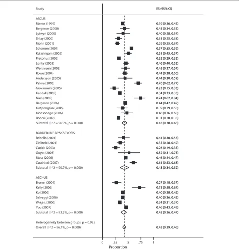
Arbyn et al. [17] assessed the HPV test positivity rate in women with equivocal or low-grade cervical cytolog-ical abnormalities. HPV testing has been proposed as a method to triage women with minor cytological abnor-malities identified through screening for cervical cancer using the Pap smear [19,20]. The prevalence of HPV infec-tion reflects the burden of referral and diagnostic work-up when the test is used to triage women with these cyto-logical conditions [17]. Two groups of minor cytocyto-logical abnormalties can be distinguished: a) atypical squamous cells of undetermined significance (ASC-US) or border-line dyskaryosis and b) low-grade squamous intraepithe-lial lesion (LSIL) or mild dyskaryosis. The meta-analysis concluded that the large majority of women with LSIL were infected with HPV suggesting limited utility of HPV triaging. However, for women with ASC-US, more than halve tested negative and could be released from further follow-up. Figure 1 reproduces the meta analysis includ-ing 32 studies providinclud-ing data of HPV infection in case of equivocal cervical cytology (ASC-US). The pooled preva-lence of HPV infection, assessed with the Hybrid Capture

2 assay was 43% (95% CI: 39%-46%) (see Figure 1 and Table 2).

The dataset contains author and year which identify each study, where tgroup corresponds with the triage group(ASCUS, LSIL, borderline dyskaryosis). num and

denom indicates the number of women with a positive HPV test (HC2 assay) and total number of tested women such that frac_denomnum is the proportion with a positive HC2 test. se indicates the standard error computed as

frac(1−frac)

denom .loandupare the lower and upper confidence

intervals computed using the ‘exact’ method.

Dataset two

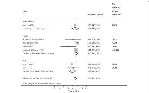
Dolman et al. [18] published a systematic review on the efficacy of cold coagulation to treat cervical intraepithe-lial neoplasia (CIN). Thirteen reports were included in the meta-analysis which showed a high degree of hetero-geneity among studies. Several studies had cure rates at or close to 100%. As seen in Figure 2, the Wald confidence intervals yield values beyond 1 for some of the individ-ual studies and for the pooled proportion for studies conducted in Europe.

The dataset containsnb_curedandnb_treatedindicates the number of women cured of CIN and total number of women treated for CIN such that frac_nbnb_{_}__treatedcuredis the proportion of women cured of CIN, and se is the stan-dard error.regionindicates continent in which the study was conducted. For studies withfrac=1,se=0 and the authors replacedse= up_2∗1.96low, whereupandlowwere the exact binomial confidence intervals to ensure that such studies were not excluded from the analysis.

Software development

The metaprop command is an adaptation of the metan programme developed by Harris et al. [10] intended to perform fixed and random-effects meta-analysis in Stata on continuous variables or associations between continuous or binomial variables. The metaprop pro-gram and its help file are available for download-ing at http://ideas.repec.org/c/boc/bocode/s457781.html. The command requires Stata 10 or later versions and can be directly installed within Stata by typing ssc install metapropwhen one is connected to the internet. An update to metaprop to include the logistic-normal random-effects model is also available for download. The updated command metaprop_one requires Stata 13 and can be directly installed within Stata by typingssc install metaprop_onewhen one is connected to the internet.

Results Example one

We reproduce Figure one in Arbyn et al. [17].metaprop

Heterogeneity between groups: p = 0.925 Overall (I^2 = 96.1%, p = 0.000); Guyot (2003)

Zielinski (2001) Bergeron (2006) Morin (2001)

Giovannelli (2005) Lonky (2003) Lytwyn (2000)

You (2007) Bruner (2004) Kendall (2005)

ASC−US

Subtotal (I^2 = 90.7%, p = 0.000) Manos (1999)

Cuschieri (2007) Cuzick (2003) Kiatpongsan (2006) Solomon (2001)

Kelly (2006) Nieh (2005)

Subtotal (I^2 = 96.9%, p = 0.000)

Wright (2006) Wensveen (2003)

Monsonego (2006)

Moss (2006) Study

Ronco (2007)

Ko (2006) Andersson (2005) Palma (2005)

Subtotal (I^2 = 93.2%, p = 0.000) Pretorius (2002)

BORDERLINE DYSKARYOSIS Kulasingam (2002)

Rebello (2001) Rowe (2004) Shlay (2000)

Selvaggi (2006) Bergeron (2000) ASCUS

0.43 (0.39, 0.46) 0.52 (0.31, 0.73) 0.35 (0.28, 0.42) 0.44 (0.42, 0.47) 0.29 (0.25, 0.34)

0.23 (0.15, 0.33) 0.46 (0.40, 0.52) 0.40 (0.28, 0.54)

0.46 (0.43, 0.49) 0.27 (0.18, 0.37) 0.34 (0.33, 0.35)

0.43 (0.34, 0.52) 0.39 (0.36, 0.43)

0.61 (0.53, 0.68) 0.26 (0.19, 0.35) 0.39 (0.29, 0.50) 0.57 (0.55, 0.59)

0.73 (0.58, 0.84) 0.74 (0.62, 0.84)

0.43 (0.38, 0.48)

0.34 (0.31, 0.37) 0.45 (0.37, 0.54)

0.48 (0.36, 0.60)

0.46 (0.44, 0.47) ES (95% CI)

0.31 (0.28, 0.35)

0.40 (0.38, 0.42) 0.44 (0.30, 0.59) 0.70 (0.62, 0.77)

0.42 (0.36, 0.47) 0.32 (0.29, 0.35) 0.51 (0.45, 0.57)

0.41 (0.30, 0.53) 0.44 (0.38, 0.50) 0.31 (0.25, 0.38)

0.40 (0.36, 0.43) 0.43 (0.34, 0.53)

0.43 (0.39, 0.46) 0.52 (0.31, 0.73) 0.35 (0.28, 0.42) 0.44 (0.42, 0.47) 0.29 (0.25, 0.34)

0.23 (0.15, 0.33) 0.46 (0.40, 0.52) 0.40 (0.28, 0.54)

0.46 (0.43, 0.49) 0.27 (0.18, 0.37) 0.34 (0.33, 0.35)

0.43 (0.34, 0.52) 0.39 (0.36, 0.43)

0.61 (0.53, 0.68) 0.26 (0.19, 0.35) 0.39 (0.29, 0.50) 0.57 (0.55, 0.59)

0.73 (0.58, 0.84) 0.74 (0.62, 0.84)

0.43 (0.38, 0.48)

0.34 (0.31, 0.37) 0.45 (0.37, 0.54)

0.48 (0.36, 0.60)

0.46 (0.44, 0.47) ES (95% CI)

0.31 (0.28, 0.35)

0.40 (0.38, 0.42) 0.44 (0.30, 0.59) 0.70 (0.62, 0.77)

0.42 (0.36, 0.47) 0.32 (0.29, 0.35) 0.51 (0.45, 0.57)

0.41 (0.30, 0.53) 0.44 (0.38, 0.50) 0.31 (0.25, 0.38)

0.40 (0.36, 0.43) 0.43 (0.34, 0.53)

0 .25 .5 .75 1

Proportion

Figure 1Meta-analysis of the proportion of women with ASCUS or a borderline Pap smear that have a positive Hybrid Capture II test.

Output generated by the Stata proceduremetaprop.

overall pooled estimates with inverse-variance weights obtained from a random-effects model.

. metaprop num denom, random by(tgroup)

cimethod(exact) /*

*/ label(namevar=author, yearvar=year) /* */ xlab(.25,0.5,.75,1)xline(0, lcolor(black)) /* */ subti(Atypical cervical cytology, size(4)) /* */ xtitle(Proportion,size(2)) nowt /*

*/ olineopt(lcolor(red)lpattern(shortdash))/* */ plotregion(icolor(ltbluishgray)) /*

*/ diamopt(lcolor(red)) /*

*/ pointopt(msymbol(x)msize(0))boxopt(msymbol(S) mcolor (black)) /*

Table 2 Meta-analysis of the presence of high-riskHPVDNAin women with equivocal cervical cytology, by terminology group (ASCUS,Borderline Dyskaryosis orASC-US)

Study ES [95% Conf. interval]

ASCUS

Manos (1999) 0.395 0.364 0.426

Bergeron (2000) 0.432 0.339 0.53

Lytwyn (2000) 0.404 0.276 0.542

Shlay (2000) 0.313 0.248 0.383

Morin (2001) 0.292 0.245 0.342

Solomon (2001) 0.568 0.547 0.588

Kulasingam (2002) 0.511 0.45 0.572

Pretorius (2002) 0.322 0.293 0.353

Lonky (2003) 0.46 0.401 0.521

Wensveen (2003) 0.453 0.371 0.537

Rowe (2004) 0.44 0.38 0.501

Andersson (2005) 0.442 0.305 0.587

Palma (2005) 0.699 0.62 0.769

Giovannelli (2005) 0.228 0.147 0.328

Kendall (2005) 0.341 0.33 0.352

Nieh (2005) 0.742 0.62 0.842

Bergeron (2006) 0.444 0.422 0.467

Kiatpongsan (2006) 0.389 0.288 0.497

Monsonego (2006) 0.479 0.359 0.601

Ronco (2007) 0.314 0.281 0.349

Sub-total

Random pooled ES 0.431 0.382 0.480

BORDERLINE DYSKARYOS

Rebello (2001) 0.413 0.301 0.533

Zielinski (2001) 0.347 0.284 0.415

Cuzick (2003) 0.26 0.185 0.347

Guyot (2003) 0.522 0.306 0.732

Moss (2006) 0.456 0.44 0.473

Cuschieri (2007) 0.605 0.532 0.675

Sub-total

Random pooled ES 0.428 0.341 0.516

ASC-US

Bruner (2004) 0.269 0.182 0.371

Kelly (2006) 0.725 0.583 0.841

Ko (2006) 0.401 0.381 0.421

Selvaggi (2006) 0.396 0.359 0.434

Wright (2006) 0.341 0.315 0.368

You (2007) 0.463 0.434 0.492

Sub-total

Random pooled ES 0.416 0.360 0.472

Overall

Table 2 Meta-analysis of the presence of high-riskHPVDNAin women with equivocal cervical cytology, by terminology group (ASCUS,Borderline Dyskaryosis orASC-US)(Continued)

Test(s) of heterogeneity:

Heterogeneity statistic Degrees of freedom p-value I2∗∗

ASCUS 614.42 19 0.000 96.9%

BORDERLINE DYSKARYOS 53.58 5 0.000 90.7%

ASC-US 73.92 5 0.000 93.2%

Overall 785.77 31 0.000 96.1%

Random: Rest for heterogeneity between sub-groups:

0.16 2 0.925

**I2: the variation in ES attributable to heterogeneity

Significance of test(s) of ES = 0

ASCUS z = 17.22 p = 0.000

BORDERLINE

DYSKARYOS z = 9.58 p = 0.000

ASC-US z = 14.57 p = 0.000

Overall z = 25.31 p = 0.000

Output generated by the Stata proceduremetaprop.

with 95% Wald confidence intervals and the I2 statis-tic which describes the percentage of total variation due to inter-study heterogeneity. The table presents addi-tional information on the pooled proportions and includes tests of heterogeneity within the sub-groups and over-all. Significant intra-group heterogeneity was observed (p<0.001 withI2exceeding 93% for all the three terminol-ogy groups). However, no inter-group heterogeneity was noted (p =0.925), supporting the pooling of all studies into one pooled measure: 43% (95% CI: 39-46%).

Though the weights have been computed using the random-effects model, the heterogeneity statistics have been computed by re-calculating the overall pooled esti-mate by treating the sub-group pooled estiesti-mates as though they were fixed-effects estimates. Since all study-specific proportions are close to 0.5,metan(see Figure one in Arbyn et al. [17]) andmetaprop(see Figure 1) produce similar results.

Example two

We extracted data that generated Figure two in Dolman et al. [18] (see Figure 2). Since the proportion of cured women is close to or at 1 in some studies, we enabled the Freeman-Tukey double arcsine transformation. Oth-erwise, studies with estimated proportion at 1 would be excluded from the analysis leading to a biased pooled esti-mate. Alternatively; usingcc(#) ensures that such studies are not excluded. However, the pooled estimate is not guaranteed to be within the [0,1] interval which is auto-matic when the Freeman-Tukey double arcsine(ftt) option is enabled. We used the score confidence intervals for the individual studies.

. metaprop nb_cured nb_treated, random by(region) ftt cimethod(score)/*

*/ label(namevar = study) graphregion(color(white)) plotregion(color(white))/*

*/ xlab(0.5,0.6,.7,0.8, 0.9, 1) /* */ xtick(0.5,0.6,.7,0.8, 0.9, 1) force/* */ xtitle(Proportion,size(2)) nowt stats /* */ olineopt(lcolor(black) lpattern(shortdash)) /* */ diamopt(lcolor(black)) /*

*/ boxopt(msymbol(S)) rcols(col)/* */ astext(70) texts(80) nohet notable

Figure 3 (displaying the forest plot generated by

metaprop) presents the study-specific proportions with 95% score confidence intervals, the regional and overall pooled estimates with 95% Wald confidence intervals,I2

statistic, and test of significance of the overall pooled esti-mates. In contrast with Figure 2 (displaying the graphical output generated withmetan), all the confidence intervals have admissible values.

Example three

NOTE: Weights are from random effects analysis .

.

.

Overall (I−squared = 42.5%, p = 0.107) Joshi (2013)

Loobuyck & Duncan (1993)

Subtotal (I−squared = 51.6%, p = 0.102)

Asia North America

Europe

de Cristofaro (1990) Study

Javaheri (1981)

Hussein & Galloway (1985) ID

Subtotal (I−squared = .%, p = .)

Singh (1998)

Subtotal (I−squared = 0.0%, p = 0.746) Rogstad (1992)

0.96 (0.92, 0.99) 0.91 (0.79, 1.03) 0.97 (0.95, 0.99)

0.97 (0.93, 1.01) 1.00 (0.96, 1.04) 0.96 (0.87, 1.04)

0.91 (0.74, 1.08) Proportion (95% CI)

0.96 (0.87, 1.04)

0.88 (0.79, 0.98)

0.89 (0.82, 0.97) 0.80 (0.62, 0.98)

20/22 cured/Nb

445/459 Nb

42/42 treated

22/23

10/11 with F−Up

38/43 16/20

0.96 (0.92, 0.99) 0.91 (0.79, 1.03) 0.97 (0.95, 0.99)

0.97 (0.93, 1.01) 1.00 (0.96, 1.04) 0.96 (0.87, 1.04)

0.91 (0.74, 1.08) Proportion (95% CI)

0.96 (0.87, 1.04)

0.88 (0.79, 0.98)

0.89 (0.82, 0.97) 0.80 (0.62, 0.98)

20/22 cured/Nb

445/459 Nb

42/42 treated

22/23

10/11 with F−Up

38/43 16/20

.5 .6 .7 .8 .9 1 1.1 1.2

Proportion

Figure 2Proportion-cured estimates associated with cold coagulation treatment for CIN1 disease, by world region as analysed bymetan.

. metaprop_one nb_cured nb_treated, random logit groupid(study) ///

label(namevar=author, yearvar=year) sortby(year author) /// xlab(.1,.2,.3,.4,.5,.6,.7,.8,.9,1) xline(0, lcolor(black)) /// ti(Positivity of p16 immunostaining, size(4) color(blue)) /// subti("Cytology=HSIL", size(4) color(blue)) /// xtitle(Proportion,size(3)) nowt nostats /// olineopt(lcolor(red) lpattern(shortdash)) ///

diamopt(lcolor(red)) pointopt(msymbol(s) msize(2)) /// astext(70) texts(100)

Table 3 presents the study-specific proportions with 95% exact confidence intervals and overall pooled estimates with 95% Wald confidence intervals with logit transformation and back transformation,Chi2_{statistic of} Likelihood ratio (LR) test comparing the random- and fixed-effects model, the estimated between-study vari-ance and test of significvari-ance testing if the estimated pro-portion is equal to zero. The P-value for the LR is 0.022 indicating presence of significant heterogeneity. From the previous command, the Q-statistic is analogous to the LR statistic. In contrast with Figure 2 (displaying the graphical output generated with metan), all the confidence inter-vals have admissible values. The estimated pooled mean and the corresponding 95% intervals are similar to those obtained earlier (see Figure 2) computed as a weighted average after the arcsine transformation. However, the

estimated between-study variance is larger (0.4907) than the Dersimonian and Laird variance estimate obtained from the previous command (0.0409) as expected [9].

Discussion

We have presented procedures to perform meta-analysis of proportions in Stata. We adapted and made

addi-tions to the metan command to provide procedures

which are specific for binomial data where the user specifies n and N denoting the number of individuals with the characteristic of interest and the total num-ber of individuals. With metaprop, it is possible to perform a test of heterogeneity between groups when sub-group analysis is desired and the random-effects model has been used to compute the pooled estimate. In metan, a test for intergroup comparison is only pro-duced when the fixed effects model is used in a subgroup meta-analysis.

Overall Subtotal Subtotal

Subtotal de Cristofaro (1990)

Joshi (2013) Asia Rogstad (1992)

Singh (1998) Europe

Hussein & Galloway (1985)

Loobuyck & Duncan (1993) Javaheri (1981)

North America Study

0.95 (0.88, 0.99) 0.96 (0.87, 1.00) 0.96 (0.79, 0.99)

0.89 (0.80, 0.96) 1.00 (0.92, 1.00)

0.91 (0.72, 0.97) 0.80 (0.58, 0.92)

0.88 (0.76, 0.95) 0.91 (0.62, 0.98)

0.97 (0.95, 0.98) 0.96 (0.79, 0.99) ES (95% CI)

treated

42/42

20/22 Nb

cured/Nb

16/20

38/43 10/11

445/459 22/23 with F−Up

0.95 (0.88, 0.99) 0.96 (0.87, 1.00) 0.96 (0.79, 0.99)

0.89 (0.80, 0.96) 1.00 (0.92, 1.00)

0.91 (0.72, 0.97) 0.80 (0.58, 0.92)

0.88 (0.76, 0.95) 0.91 (0.62, 0.98)

0.97 (0.95, 0.98) 0.96 (0.79, 0.99) ES (95% CI)

treated

42/42

20/22 Nb

cured/Nb

16/20

38/43 10/11

445/459 22/23 with F−Up

0 .5 .6 .7 .8 .9 1

Proportion

Figure 3Proportion-cured estimates associated with cold coagulation treatment for CIN1 disease, by world region as analysed by

metaprop.

that the studies are retained, the confidence intervals for the pooled estimate may yield inadmissible values.

Furthermore, use of Wald confidence intervals for the individual studies when the estimated proportion is close to zero often yields inadmissible values. This is because the Wald confidence intervals are always symmetric around an estimate. In contrast to the Wald, the exact

or score confidence intervals can be asymmetric espe-cially near the extreme values. By computing the exact or score confidence intervals for the individuals studies, we are guaranteed of admissible values. While the exact confidence are regarded as the ‘gold’ standard, we rec-ommend the use of score confidence intervals because the coverage is close to the nominal level, whereas the

Table 3 Meta-analysis of the presence proportion of women cured ofCIN1 disease with cold coagulation)

Study ES [95% Conf. Interval]

Javaheri (1981) 0.957 0.7901 0.9923

Hussein & Galloway (1985) 0.909 0.6226 0.9838

de Cristofaro (1990) 1.000 0.9162 1.0000

Rogstad (1992) 0.800 0.5840 0.9193

Loobuyck & Duncan (1993) 0.969 0.9495 0.9817

Singh (1998) 0.884 0.7552 0.9493

Joshi (2013) 0.909 0.7219 0.9747

Random pooled ES 0.942 0.8855 0.9715

LR test: RE vs FE Modelchi2_{=4.04 (d.f.=1) p=0.022.}

Estimate of between-study varianceTau2_=0.4907.

Test of ES=0 : z=45.56 p=0.000.

coverage is always higher than the nominal level for the exact method. By using the Freeman-Tukey double arcsine transformation, all the studies are retained, furthermore, we are guaranteed to have admissible confidence inter-vals for each individual study as well as for the pooled proportion. While the distribution of the Freeman-Tukey double arcsine statistic is more normal for sparse data, the procedure breaks down with extremely sparse data and should thus be used with caution [21]. Whenever possi-ble the use of exact methods is more recommended for binomial data. As the sample size increases and when the proportions are not extreme, methods relying on trans-formed data and exact methods give similar results as approximate methods.

Conclusion

metaprop enables epidemiologists to pool proportions in Stata, avoiding problems encountered with metan.

metaprop allows inclusion of studies with proportions equal to zero or 100 percent, and avoids confidence inter-vals exceeding the 0 to 1 range. The logistic-normal random-effects model draws the users a step closer towards the use of exact methods recommended for bino-mial data.

Competing interests

The authors declare that they have no competing interests.

Authors’ contributions

VN wrote the metaprop program in Stata, analysed the data and drafted manuscript. MA* conceptualized and initiated the project and edited the manuscript. MA edited the manuscript. All authors reviewed and approved the final manuscript.

Acknowledgements

Financial support was received from: (1) the 7th Framework Programme of DG Research of the European Commission through the COHEAHR Network (grant No. 603019, coordinated by the Vrije Universiteit Amsterdam, the Netherlands) and the HPV-AHEAD project (FP7-HEALTH-2011-282562, coordinated by IARC, Lyon, France); (3) The Scientific Institute of Public Health (Brussels, through the OPSADAC project).

Author details

1_{Unit of Cancer Epidemiology, Scientific Institute of Public Health, Juliette}

Wytsmanstraat 14, 1050 Brussels, Belgium.2_{Center for Statistics, Hasselt} University, Agoralaan Building D, 3590 Diepenbeek, Belgium.

Received: 5 May 2014 Accepted: 11 July 2014 Published: 10 November 2014

References

1. Agresti A, Coull BA:Approximate is better than ’exact’ for interval estimation of binomial proportions.Am Stat1998,52(2):119–126. 2. Breslow NE, Clayton DG:Approximate inference in generalized linear

mixed models.J Am Stat Assoc1993,88:9–25.

3. Miller JJ:The inverse of the Freeman-Tukey double arcsine transformation.Am Stat1978,32(4):138.

4. Hamza TH, van Houwelingen HC, Stijnen T:The binomial distribution of meta-analysis was preferred to model within-study variability.

J Clin Epidemiol2008,61:41–51.

5. Molenberghs G, Verbeke G, Iddib S, Demétrio CGB:A combined beta and normal random-effects model for repeated, over-dispersed binary and binomial data.J Multivar Anal2012,111:94–109.

6. DerSimonian R, Laird N:Meta-analysis in clinical trials.Control Clin Trials 1986,7:177–188.

7. Engel E, Keen A:A simple approach for the analysis of generalized linear mixed models.Stat Neerl1994,48:1–22.

8. Molenberghs G, Verbeke G, Demétrio CGB, Vieira AMC:A family of generalized linear models for repeated measures with normal and conjugate random effects.Stat Sci2010,3:325–347.

9. Jackson D, Bowden J, Baker R:How does the Dersimonian and Laird procedure for random effects meta-analysis compare with its more efficient but harder to compute counterparts?J Stat Plan Inference 2010,140:961–970.

10. Harris R, Bradburn M, Deeks J, Harbord R, Altman D, Sterne J:metan: fixed- and random-effects meta-analysis.Stata J2008,8(1):3–28. 11. Box GEP, Hunter JS, Hunter WG:Statistics for experimenters. Hoboken (NJ),

USA: J Wiley & Sons Inc, Wiley Series in Probability and Statistics; 1978. 12. Freeman MF, Tukey JW:Transformations related to the angular and

the square root.Ann Math Stats1950,21(4):607–611.

13. Clopper CJ, Pearson ES:The use of confidence or fiducial limits illustrated in the case of the binomial.Biometrika1934,26(4):404–413. 14. Brown LD, Cai TT, DasGupta A:Interval estimation for a binomial

proportion.Stat Sci2001,16:404–413.

15. Newcombe RG:Two-sided confidence intervals for the single proportion: comparison of seven methods.Stat Med1998,17:857–872. 16. Wilson EB:Probable inference, the law of succession, and statistical

inference.J Am Stat Assoc1927,22(158):209–212.

17. Arbyn M, Martin-Hirsch P, Buntinx F, Ranst MV, Paraskevaidis E, Dillner J:

Triage of women with equivocal or low-grade cervical cytology results a meta-analysis of the hpv test positivity rate.J Cell Mol Med 2009,13(4):648–659.

18. Dolman L, Sauvaget C, Muwonge R, Sankaranarayanan R:Meta-analysis of the efficacy of cold coagulation as a treatment method for cervical intra-epithelial neoplasis: a systematic review.BJOG2014,

121:929–942.

19. Arbyn M, Ronco G, Anttila A, Meijer CJLM, Poljak M, Ogilvie G, Koliopoulos G, Naucler P, Sankaranarayanan R, Petok J:Evidence regarding human papillomavirus testing in secondary prevention of cervical cancer.

Vaccine2012,30(Suppl 5):F88–F99.

20. Arbyn M, Roelens J, Simoens C, Buntinx F, Paraskevaidis E, Martin-Hirsch PP, Prendiville WJ:Human papillomavirus testing versus repeat cytology for triage of minor cytological cervical lesions.Cochrane Database Syst Rev2013,3(CD008054):1–201.

21. Westfall PH, Young SS:Resampling-based multiple testing: examples and methods for P-value adjustment. Hoboken (NJ), USA: John Wiley & Sons; 1993.

doi:10.1186/2049-3258-72-39

Cite this article as:Nyagaet al.:Metaprop: a Stata command to perform meta-analysis of binomial data.Archives of Public Health201472:39.

Submit your next manuscript to BioMed Central and take full advantage of:

• Convenient online submission

• Thorough peer review

• No space constraints or color figure charges

• Immediate publication on acceptance

• Inclusion in PubMed, CAS, Scopus and Google Scholar

• Research which is freely available for redistribution