Investigating and modelling the interaction among vegetation, hydrodynamics and morphology

(1)

1

Do ctoral Studies in

Environmental Engineering

Erasmus Mundus Joint Doctorate School in Science for MAnagement of Rivers and their Tidal System

Politti Emilio

(2)

November, 2017

Doctoral thesis in Science for MAnagement of Rivers and their Tidal System, IV Cohort

University of Trento - Department of Civil, Environmental and Mechanical Engineering Queen Mary University of London – School of Geography

Edmund Mach Foundation Supervisors

Walter, Bertoldy, University of Trento

Alexander J., Henshaw, Queen Mary University of London

(3)

3

The SMART Joint Doctorate Programme

Research for this thesis was conducted with the support of the Erasmus Mundus Programme1, within the framework of the Erasmus Mundus Joint Doctorate (EMJD) SMART (Science for MAnagement of Rivers and their Tidal systems). EMJDs aim to foster cooperation between higher education institutions and academic staff in Europe and third countries with a view to creating centres of excellence and providing a highly skilled 21st century workforce enabled to lead social, cultural and economic developments. All EMJDs involve mandatory mobility between the universities in the consortia and lead to the award of recognised joint, double or multiple degrees.

The SMART programme represents a collaboration among the University of Trento, Queen Mary University of London, and Freie Universität Berlin. Each doctoral candidate within the SMART programme has conformed to the following during their 3 years of study:

(i) Supervision by a minimum of two supervisors in two institutions (their primary and secondary institutions).

(ii) Study for a minimum period of 6 months at their secondary institution (iii) Successful completion of a minimum of 30 ECTS of taught courses

(iv) Collaboration with an associate partner to develop a particular component / application of their research that is of mutual interest.

(v) Submission of a thesis within 3 years of commencing the programme.

(4)

Acnowledgements

(5)

5

Abstract

Abstract

The dissertation presented in this manuscript contributes to river science by providing a detailed overview on the state of the art on the interaction between riparian vegetation and hydrogeomorphological processes, by devising a novel model encompassing most of such processes and by proposing a field methodology aimed at providing means for improving the modelling of such interactions. The state of the art is summarized in an extensive review describing riparian vegetation and hydrogeomorphological processes mutual feedbacks. Such review did not simply seek to describe these feedbacks but, compiling from a large array of results from field, laboratory and modelling studies, provides a set of physical thresholds that trigger system changes. Therefore, processes are not only described terms but also explained with a quantitative approach. Processes description provided the conceptual foundation for the development of the novel simulation model while model parameterization was based on the quantitative information collected in the review. Such novel model, encompasses the main relationships entwining riparian woody vegetation and hydrogeomorphological processes and is able of replicating long term riparian landscape dynamics considering disturbance events, environmental stressor and riparian woody vegetation establishment from seeds and large wood. The manuscript presents the model structure and its conceptual validation by means of hydrological scenarios aimed at testing the coherence of the simulation results with expected system behaviour. Examples of such coherences are vegetation growth rate in response to hydrological regime, entrainment and establishment of large wood in an unconfined river system and vegetation effect on erosion and deposition patterns.

(6)

List of Figures

Figure 1-1 Process hierarchy of vegetation feedbacks to fluvial processes ..25 Figure 1-2 Process hierarchy of fluvial process feedbacks to vegetation ...25

Figure 1-3 Tensile strength per unit area calculated for three species of Salicaceae with Eq. 1. Data sources: (Pollen and Simon, 2005; Polvi et al., 2014; Simon et al., 2006) 26 Figure 1-4 Modelled Populus fremontii and Salix nigra increase in soil cohesion in

relation to age. Data source: (Pollen-Bankhead and Simon, 2009). ...29

Figure 1-5 Effects of a finite width patch on the flow field horizontal dimension. Adapted from (Nepf, 2012) ...31

Figure 1-6 Effects of a circular patch on the flow field horizontal dimension. Adapted from (Nepf, 2012) ...31

Figure 1-7 Effects on the flow field vertical distribution of a submerged (A) and partially submerged (B) patch. Adapted from (Baptist et al., 2009) and (Nepf and Vivoni, 2000) ...32

Figure 1-8 Scour and deposition measured in a flume experiment, for a channel side and a centre bar with flexible objects simulating flexible submerged vegetation. Scour was measured upstream and on the sides of the bars, deposition was measured downstream from the bars. Plant density is the ratio of the projected area of the flexible objects and the area of each bar. In the charts, a plant density of 1 indicates a solid, non-flexible object with the same bar area and object height as that of the flexible objects. Data source: Chen, Kuo & Yen 2012b ...33

Figure 1-9 Survival of seed-recruited seedlings under different water table decline rates (Data source: Table 1-5) ...34

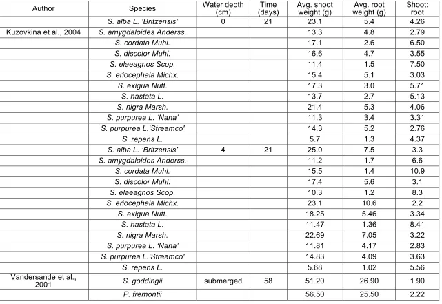
Figure 1-10 Mean shoot (top) and root (bottom) weight percentage variations in response to inundation (flooding depth and duration varies; see Table 1-6) ...40

Figure 1-11 Mortality of Salix spp. cuttings due to deposition, erosion and shear stress (Pasquale et al., 2014) ...41

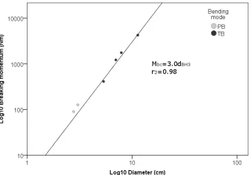
Figure 1-12 Relationship between breaking momentum and trunk diameter for S.

subfragilis from laboratory experiments. PB: Plastic Bending, TB: Trunk Breakage (adapted from Tanaka and Yagisawa, 2009) ...43

Figure 1-13 Relationship between the dimensionless particle shear stress and

dimensionless critical particle shear stress and morphodynamic bending effects (with τ*84 dimensionless shear stress acting on d84 particle size, τ*c84

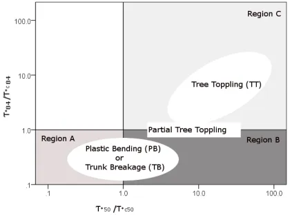
dimensionless critical shear stress for d84 particle size motion, τ*50 dimensionless shear stress acting on d50 particle size, τ*c50 dimensionless critical shear stress for d50 particle size motion). Region A: quasi-clear scour: only particles smaller than d50 are mobilized. Region B: bed partial scour: particles in the range of the d50 are entrained, possibly causing local armouring. Region C: bed scour: particles in the range of the d84 are entrained, thus causing local erosion. Adapted from Tanaka & Yagisawa (2009) ...45

Figure 1-14 Relative burial percentage and survivorship of 1-3 years old seedlings of Populus fremontii with heights ranging from 14 to 69 cm. Data extracted from Kui & Stella (2016) ...47

Figure 1-15 Relevant water stage thresholds and time scales affecting riparian Salicaceae recruitment, growth and survival ...51

(9)

9

Figure 2-2 CLF and RVM submodels and feedbacks integration schema ...64

Figure 2-3 Conceptualization of deposition effect on RDMD and plants' height. RDMD: root density maximum depth, H: plant height, d: deposition, b: bending angle resulting from deposition ...68 Figure 2-4 Initial vegetation distribution derived for the simulated reach ...73

Figure 2-5 Normal flow regime (A) and Sustained low flows scenarios (B) hydrographs used to test flow regime feedback to vegetation growth performance ....74

Figure 2-6 Hydrograph of a Tagliamento 10 year recurrence interval flood used to simulate vegetation feedback to sediment transport processes ...75 Figure 2-7 Initial vegetation for the LW lifecycle test case ...77 Figure 2-8 Hydrograph used to simulate LW recruitment and establishment 77

Figure 2-9 Cumulative biomass in the modelling domain pixels vegetated at the beginning of the undrying and drying scenarios ...78

Figure 2-10 Total vegetation biomass for the undrying and undrying scenarios 79 Figure 2-11 Vegetated area in the drying and undrying scenarios ...79

Figure 2-12 Vegetation age distribution of the last simulated year of the Sustained low flow scenario scenario ...80

Figure 2-13 Vegetation age distribution of the last simulated year of the Normal flow regime ...80

Figure 2-14 Eroded and deposited sediment volumes in the areas covered by vegetation in the vegetated and unvegetated scenarios ...81

Figure 2-15 Erosion, deposition and stable areas of the vegetated areas for the vegetated and unvegetated scenarios ...82

Figure 2-16 LW deposition positions after the first simulated year ...83 Figure 2-17 A: potential LW sources before the 1st year May flood. B: potential LW

sources after the 1st year May flood and LW stranding locations ...84

Figure 2-18 A: potential LW sources before the 1st year November flood. B: potential LW sources after the 1st year November flood and LW stranding locations .85

Figure 2-19 Erosion and deposition at the stranding locations of the LW entrained during the 1st year floods ...86

Figure 2-20 Resprouting wood deposited by the first year flood events ...86

Figure 2-21 Stranding elevation above the detrended topography of the first simulated year ...89

Figure 2-22 1st year survival elevation above the detrended topography of the first simulated year ...89

Figure 2-23 A: Median particle size (D50) of the 2nd simulated year, in the locations where LW deposited in the 1st year resprouted. B: D50 of the 2nd simulated year in

locations where LW depositions did not occur. ...91

Figure 2-24 A: histogram of the median particle size (D50) of the second simulated year. B: boxplot of the median particle size (D50) of the second simulated year. 92

(10)

Figure 2-26 Side channel filling observed on the Tagliamento upstream from the modelled site. Blue arrow on 2003 image indicates the flow direction ...95

Figure 3-1 Graphical representation of the leaf are sampling performed by placing the camera at different heights. On the top rows, examples of resulting HPs in foliated and defoliated conditions. Note how gap fraction increases as camera position heightens. ...188

Figure 3-2 Shape and position of the vegetation in the two modelled scenarios. In both scenarios, flow direction goes from the left edge to the right one. ...192

Figure 3-3 Measured values of PAI, STAI and FAI, and interpolation lines, as a function of the relative height ...194

Figure 3-4 Friction factors modelled and yield from direct measures on fully submerged specimens. Modelled friction factors are computed assuming a complete

submersion, using Equation 18 and Equation 19 to compute FAI and LAI and Equation 1 to compute friction factor. SC: Salix Caprea, SR: Salix Rubens, MW: Mountain Willow, HW: Hybrid Willow, SV: Salix Viminalis, SCL: Salix Caprea Low, SCH: Salix Caprea High. Image in colour available online ...196

Figure 3-5 Friction factors calculated with Equation 1 assuming foliated and defoliated condition and different flow velocities. Legend entries ending with “F” represent Foliated conditions, while those ending with “D” Defoliated conditions. Empirical parameters acronyms: Salix Caprea (SC), Salix Caprea Low (SCL), Salix Caprea High (SCH), Salix Rubens (SR), Salix Viminalis (SV). ...197

Figure 3-6 Sensitivity to LAI and FAI of Equation 1 applied with Salix rubens parameters. Red dotted line represents the friction factor value calculated without any variation ...199

Figure 3-7 Chart in the left column depict the ratio between the water depth simulated using Equation 1 and the water depths using fixed Manning’s coefficients. Charts in the left column are instead the value of Manning’s n. In the charts of both columns, the x axis represents the x coordinate on the longitudinal dimension of the vegetated bank. Manning’s n fixed values: 0.045 (VBN0045), 0.062 (VBN0062) and 0.098

(VBN0098). VBSRF: Salix Rubens Foliated, VBSRD: Salix Rubens Defoliated. 201 Figure 3-8 Left column contains boxplots of the rate between bed shear stress modelled

with Equation 1, in foliated conditions and using SR parameters and the bed shear stress modelled in defoliated conditions and with a fixed roughness. X axis entries marked with “IS” represent the bed shear stress values inside the centre island, while those unmarked are yield from the bulk of shear stress values in the analysis reach. Right column contains the boxplots of the Manning’s n coefficients inside the centre island. Manning’s n fixed values: 0.045 (CIN0045), 0.062 (CIN0062) and 0.098 (CIN0098). CISRF: Salix Rubens Foliated, CISRD: Salix Rubens Defoliated. 203 Figure 3-9 Bed shear stress in the analysis reach at full submersion. Flow direction is

(11)

11

List of Tables

Table 1-1 Roots reinforcement estimated by RipRoot model for a bank 10 m long and a shear surface length of 1.15 m (Pollen and Simon, 2005) ...28

Table 1-2 Maximum groundwater depth for survival of Populus and Salix species (expanded from Lite and Stromberg, 2005) ...37 Table 1-3 Groundwater depth thresholds and corresponding timescales affecting

Salicaceae processes ...38

Table 1-4 Percentiles of the pullout forces measured on seedlings with different root frontal area and rooted in different substrates. Seedlings rooted in finer sediments generally exhibit higher pullout forces because of the higher friction due to the larger roots-substrate contact surface. (Data source: Bywater-Reyes et al., 2015) 44

Table 1-5 Experimental and observed water table decline rates, root elongation,

substrates and germinations survival percentages of seedlings and cuttings. * Field observation; ** Controlled experiment; *** Field experiment. W Weight, L Length. s Seedling, c Cutting ...52

Table 1-6 Shoot and root growth responses to flooding stress experiments .56 Table 1-7 Factors controlling riparian species asexual reproduction and survival.

*Asexual mode: 1flood training, 2: translocated fragments, 3: coppice re-growth, 4: suckering. * *Site specific (observed). ***From summer river stage. ****Elevation relative to nearest vegetated surface. ***** Measured with respect to the lower limit of established floodplain forest. a Field study. b Controlled experiment c Field

experiment ...59

Table 2-1 Initial vegetation properties estimated according to distance from the growing season water table ...72

Table 2-2 Allometric relationships relating height and diameter at breast height to Populus Nigra age ...73

Table 2-3 Stranding and 1st year survival percentages calculated on the total number of locations and percentage of 1st year survival per location calculated on the total stranding per location ...87

Table 2-4 Wood mass storage percentages measured on the Tagliamento in the summer of 1998 on two river reaches located immediately upstream and downstream of the modelled reach. Data extracted from Gurnell, Petts, Harris, et al., (2000)87

Table 2-5 Percentage of dead and live (resprouting) wood measured on the Tagliamento in the summer of 1998 on two river reaches located immediately upstream and downstream of the modelled reach. Data extracted from: Gurnell et al., (2000a) 88 Table 2-6 CLF and RVM inputs and units of measures. * Mandatory input ...1

Table 2-7 CLF parameters. Adapted from Ziliani et al., (2013) ...2 Table 2-8 Sediment input grain sizes and distribution (Ziliani, 2011) ...2

Table 2-9 Model parameters, their units, description, values applied in the test case and submodels by which parameters are used ...3

Table 2-10 Description of the linguistic variables, their units, direction (input or output) and submodels by which the linguistic variables are used ...5

(12)

SING: singleton. Numbers preceding the shapes shortcut mark the control points of the sets shapes. ...8

Table 2-12 Fuzzy rules applied in each submodel ...179 Table 3-1 Equation 1 empirical parameters. a Jalonen & Järvelä, (2014), b Västilä &

Järvelä (2014) ...189

Table 3-2 Scenarios-simulations, flow resistance modelling solution and corresponding acronyms ...193

(13)

13

Introduction

Introduction

Background and motivation

Mankind is depending upon freshwater availability since its early times. In the latest centuries, the dependency went far beyond the simple physiological needs: besides supplying human settlements for civil purposes, freshwater is in fact also used for manufacturing goods, processing staples, intensive agriculture and not less importantly, electricity production. All these uses put a significant pressure on water resources (Dudgeon et al., 2006); when considering rivers, in many cases (e.g. water extraction or hydro-power production) water exploitation require also the construction and operation of hydraulic works which alter the physiognomy and functionality of the riparian landscape (Azami et al., 2004; Braatne et al., 2007; Jamieson and Braatne, 2001). This set of issues raised concerns on the conservation of rivers’ good ecological status and the consequent formulation of stringent legal frameworks such as the Water Framework Directive, the Water Blueprint or the Habitat Directive (European Parliament, 2012, 2000, 1992).

In parallel with the evolution of legislative frameworks aimed to ameliorate and protect riparian habitats, also scientists’ view toward the rivers has changed. In the latest decades river studies have moved from hydrologists and limnologist approaches that considered lotic and terrestrial zones as distinct entities, to perspectives that acknowledged the tight connection between river and surrounding landscape. This new course was marked by the formulation of the Flood Pulse Concept (FPC) (Junk et al., 1989) which recognized the importance of lateral connectivity over the longitudinal one. FPC was extended by Tockner, Malard & Ward (2000) who considered also theories and concepts relating discharge and biodiversity also for temperate and periglacial rivers. In this re-formulation of the FP concept, also discharges below the bankfull (the “flow pulse”) are considered important for the creation and maintenance of the riverscape heterogeneity and biodiversity patterns. This latter work spearheaded the application of landscape ecology approaches to understand patterns and processes occurring within the “riverine landscape” (sensu Church, 2002). Such concepts were further developed in later papers (Ward et al., 2002; Wiens, 2002) where the authors considered spatial patterns, dynamic interactions and functional processes occurring across riparian zones. Riparian landscape perspectives sublimated in the “shifting mosaic concept” (Stanford et al., 2005) which postulates “…composition and abundance of habitat types do not change over time despite high habitat turnover rates”. Despite the simplicity of the concept, the implications deriving from this statement are manifold. The shifting mosaic formulation acknowledges the importance of periodic disturbance events that re-work the landscape features composition and affect vegetation growth as well as the periodic intervals at which such disturbances occur (Whited et al., 2007). Further implication is the relevance of the temporal scale required to fully characterize riparian zones. Single point observations cannot capture the temporal oscillation of the landscape features abundance since they may greatly differ within relative short periods (Figure I).

(14)

This brief review of the recent history of the funding paradigms underpinning the study of riverine landscape ecology is by no mean an extensive review of all the valuable works that contributed to the advancement of science in this field but rather an overview on how the perspectives and approaches toward the study of the riparian zones has changed through time. Contemporary river science paradigms recognize the importance of the multidirectional feedbacks occurring among biotic, physical and geomorphic components of the riparian landscape. Consequently, studying such systems requires looking at riparian ecosystems under a multifocal lens, crafted from different scientific fields. At the same time, studies must take into account the different temporal scales at which feedbacks occur as well as the long term spatio-temporal dynamics (Richards et al., 2002).

Figure I Rate between islands area and corridor area over time at the Tagliamento River (Italy). The periodic fluctuations of the two habitats illustrates the shifting mosaic concept (Arscott et al., 2002)

Riparian vegetation ecological succession and hydrogeomorphological processes

(15)

15

Table I Process types according to Egger et al. 2013, Formann et al. 2013. TRECmat*: Time Recovery mature stage

Process type Process relationships Process

Characteristics

Metastable I = R;

TDIS << TRECmat* Oscillatory and gap dynamics are observed but no real Mature stage never reached successional development takes place

Succession sequence interruption causes the biocoenosis to remain at the same early stage

Oscillation I > R;

TDIS < TREC-mat Vegetation succession is observed, but maturity is never reached Disturbance severity is high Recovery time is high

System is always in an unstable state Acyclic TDIS > TREC-mat Succession progress until the mature stage

Typical of zones rarely affected by river dynamics

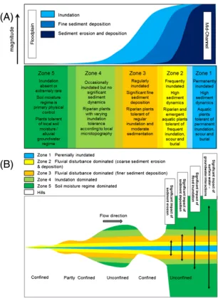
The prevailing disturbance regime, is determined by river energy gradient, aspect (width to depth ratio) and sediment size, therefore they vary according to river type (e.g. braided versus meander) and position within the active channel (Gurnell et al., 2016, 2012). On the other hand, vegetation resistance and recovery time depend on vegetation development stage. However, because of channel migration, process-types spatial arrangement can change over time and thus successional dynamics are not immutably bound to a specific location.

(16)

Figure II Characteristics of the river corridor hydromorphological zones according to inundation frequency and sediment dynamics (A) and lateral variation along the longitudinal dimension (B)

(17)

17

Table II Succession stages and phases characteristics according to Egger et al. 2013

Stage Phase Description

Colonization

Initial

Consists of bare soil where few plants are present, and in some instances seedlings only become established for a short time period

before the next disturbance

Pioneer

Relatively sparse, newly recruited vegetation. It consists primarily of species with a ruderal or stress

tolerant strategy which are adapted to frequent disturbance and strong hydrological variability

Transitional

Herb

Characterized by short-lived herbaceous species with a ruderal

or competitive strategy. In many cases, it may comprise

mono-specific vegetation of sedges and/or reeds

Shrub

Develops directly from the ‘Pioneer Phase’ or follow the ‘Herb

Phase’. It comprises woody and long-lived species with

stress-tolerant and competitive development strategies

Early Successional Woodland

Trees replace the shrubs as the dominant life forming the patch. Dominant trees were recruited

during the ‘Initial Phase’

Established Forest Phase

Species are recruited to the understory in the Early Successional Woodland Phase. They typically have slow growth rates and many may die before the onset of the next succession phase. Patches are more stable,

less prone to disturbance

Mature Stage Mature Mixed Forest Phase

Includes a combination of woody and long-lived riparian and

terrestrial species. Trees regenerate and grow without the influence of external disturbances

Both Gurnell et al., (2016) and Egger et al. (2013) approaches share some similarities and attempt to explain the result of the physical habitat-vegetation interaction as a progression of development stages characterized by the variation of dominant hydrogeomorphological processes, vegetation life stages, disturbance pressure and landforms. Nevertheless, the two theories differ for their fundamental approach: while Gurnell et al., (2016) put more focus on the geomorphic aspects of the subject, in Egger et al. (2013) the approach has a perspective leaning towards plant - ecology. Yet the two can be joined in an attempt to explain with a unifying perspective both geomorphic and vegetation trajectories along river corridors.

(18)

ground is bare although plants can occasionally establish but frequent inundations and active sediment dynamics promptly resets the succession. The pioneer phases of the woodland and reed series are typically recruited in Zone 2 (Auble and Scott, 1997). In the Northern hemisphere, riparian woody species recruited in the active channel are dominated by the Salicaceae family (Malanson, 1993). The species ascribed to this family (i.e. willows and poplars) bear a set of traits allowing them to withstand the severe fluvial disturbance regime and thus outcompete other species (Karrenberg et al., 2002). In the early life stage, although the woodland and reed series are competing for the future dominance, they do not exhibit relevant distinctive traits in terms of hydraulic and morphological interaction. Thus, hydrogeomorphic processes are dominant over vegetation dynamics (Gurnell et al., 2001) and vegetation succession is easily reset by floods of low magnitude (Asaeda and Rashid, 2012; Bendix, 1999). Zone 3 exhibits a lower disturbance frequency and magnitude than Zone 2, nevertheless it is regularly flooded and the disturbance regime is still relatively high. The succession phases found in this habitat are alternatively the shrub or the herb phase. These two phases progress from the pioneer phase and can reach their state if there is no disturbance able to obliterate newly created vegetation stands. As individuals grow in strength and size, their feedbacks to hydro-morphodynamics increase and trigger habitat autogenic processes. Therefore, transition from Zone 2 to Zone 3 is fostered by the biogeomorphic action of the vegetation. The capacity of vegetation to interact and modify the surrounding physical habitat is expressed by the term “ecosystem engineers” (Jones et al., 1994). Nevertheless, shrub and herb phases behave differently for their morphological traits differ. Reed series maintains an herbaceous aspect, when associated in dense mats, it protects the ground from erosion (Prosser et al., 1995) and favours the accumulation of silt and sand (Corenblit et al., 2009). On the other hand, the woodland series evolves with a shrubby habitus that reduces sediment transport capacity, that thus generates higher accretion rates (Corenblit et al., 2009). Sedimentation is caused by sediment particles interception by plants’ aerial structures and the perturbation of the flow field, which inside vegetated plots, tends to slow down (Anderson et al., 2006; Corenblit et al., 2007; Zong and Nepf, 2010). For both herb and shrub phases net accretion is as well facilitated by the reduction or impeded erosion caused by roots stabilization effect (De Baets et al., 2006; De Baets and Poesen, 2010). Presence of narrow-spaced patches of shrubs reduce channel widening and channel cutoffs (Tal and Paola, 2010) while sparse patches favours bifurcation (Coulthard, 2005) thus contributing to control the transition from multiple to single thread channels.

(19)

flood-19

induced strong currencies represents a suitable habitat for establishment of seedlings and smaller propagules. When several of these islands are found on contiguous locations, as they grow they can coalesce thus originating larger islands (Gurnell et al., 2001).

As the distance from the channel margins increases, Zone 4 degrades into Zone 5. In this latter zone, flooding is a very rare event; groundwater dynamics replaces hydrogeomorphic processes as main physical control over vegetation. The absence of disturbance events allows the trees recruited in the pioneer phase to grow to their full potential. Softwood forests species can last for a period of 30-50 years, after that, they begin to reach the maximum physiological age of an average Salicaceae (Egger et al., 2015; Friedman et al., 1996; Johnson et al., 1976). Individuals die back increases the light availability for the understory layer and afford the chance for other hardwood species to emerge to the canopy layer. While more softwood trees die back, the dominant species composition progressively switch to hardwood species such as Coniferous, Oaks, Alder, etc. (Hupp, 2000).

Alternatively, in Zone 4 and Zone 5, where hydric soils are present, the wetland series can replace the woodland. Wetlands are forming in oxbows resulting from meanders cutoff and in abandoned side arms. The first type is more typical in lowland rivers with low energy gradients (Hopkinson, 1992; Mitsch et al., 2012) while the latter can be found in braided and anastomosing rivers. In these locations wetland series can develop somehow similarly to the woodland series. Initial stages begin with submerged or floating sedge grasses (e.g. from the Cyperaceae, Juncaceae or Typhaceae families), as depressions fills with sediments deposited by floods and organic material, succession advances with a woody shrub phase and finally a swamp-bog forest phase (Hansen et al., 1995; Latterell et al., 2006). Alternatively, in abandoned and seldom flooded channels, wetland series can initiate by hydrophilic sedges and rapidly evolve arboreous cover (Hansen et al., 1995). In the wetland series, successional development is less obvious than in the woodland and reed ones and not all the stages are always present.

Riparian vegetation hydrodynamics and morphology numerical modelling history

Concurrently to the development of riparian landscape paradigms, the scientific community developed simulations models attempting to acknowledge the abovementioned multidirectional feedbacks occurring among biotic, physical and geomorphic components of the riparian landscape. In our opinion, spread of simulations models has been promoted also because of the lack of quantitative information and at least partial, lack of empirical laws explaining biotic and physical components feedbacks (see chapter 1). In fact, although a general consensus exists on the development trajectories and feedback direction, for many processes the quantification of the physical drivers’ intensity triggering biological responses and the relation between vegetation states and physical habitat response remains in many cases unclear. Examples of such unknowns are, for example, the inundation time required to yield plants damage or mortality, the quantity of deposited sediments that lead to plants extinction and the quantification of roots’ stabilizing effect on non-cohesive substrates (Politti et al., 2017). Lack of such information complicates management decisions and process understanding. To this end, the use of models represents a viable solution to explore scenarios or test the importance of riparian systems’ control factors.

(20)

rates. Although the results showed satisfactory agreement with observed data, the results of this model show also that the inclusion of morphodynamic disturbance would result in a more realistic outcome. Such impact was somehow included by Benjankar et al., (2011): in this model vegetation mortality is also caused by excess shear stress which is assumed as a proxy for morphodynamic activity. This latter model was extended by Garcia-Arias et al., (2011) with soil moisture dynamics, particularly relevant when modelling rivers in arid and Mediterranean climates. These models mimic vegetation development in response of hydraulic and morphological variables though did not implement any vegetation feedback to hydraulic and morphological processes.

On the other hand, hydraulic models developed at first as 1-D models able of simulating water depth and cross-sectional mean flow velocity by solving, most commonly, the Saint Venant equations. Later 2-D models integrating momentum and continuity equations on the vertical dimension, and thus able of simulating water depth and velocity on two horizontal planes, have been developed. Similarly, more advanced and computational-expensive 3-D models are able of simulating flow depths and velocities on all three dimensions. Flow velocities simulated with hydraulic models can be combined with sediment transport equations, thus allowing simultaneous simulation of river hydraulics and morphodynamics. However, hydraulic and hydrodynamics models typically used in both the industry and academic domains, account for vegetation as a static element, most commonly treated as an additional flow resistance term (Horritt and Bates, 2002).

The lack of true integration between vegetation and hydro-morphodynamic models rises also from the difference in the purpose that lead to the formulation of such models. Natural scientists are in fact, more intrigued by spatio-temporal dynamics spanning longer times than the event-scale dynamics, which is a typical interest promoting the development of hydromorphological models. Nevertheless, in latest years, the two fields are converging towards a more integrated view and several promising vegetation-hydromorphodynamic models emerged. For example, Bertoldi et al., (2014) proposed a model where vegetation growth, in terms of biomass, is controlled by the distance from the water table and its disruption by the shear stress required to mobilize substrate particles. Such critical value is linearly increased with vegetation biomass which controls with the same solution, also vegetation roughness. Presence of vegetation has therefore an effect on erosion processes by reducing flow velocity and increasing substrate cohesion. Similarly the model from Crosato and Saleh, (2011) account for flow resistance but includes also a distinction between submerged and emergent canopies. Such approach is followed also in van Oorschot et al., (2016) but besides submergence condition, vegetation flow resistance depends also on stem density, height and diameter which modelled using a logarithmic growth function. In addition to shear stress mobilization effect, in this latter model, vegetation mortality can occur also by waterlogging, desiccation, burial or scour.

(21)

21 Thesis objectives

Among the research priorities highlighted by Solari et al. (2015) and Camporeale et al., (2013) the research carried on within this dissertation did focus on the following topics:

I. Quantification of fluvial disturbance thresholds leading to vegetation extinction or disruption; II. Vegetation dynamics

III. LW interaction with geomorphic processes

IV. Improving the understanding of vegetation flexural properties on flow field and sediment transport dynamics

Considering these four research topics, this dissertation developed these three objectives:

1. Quantitative review of riparian Salicaceae and fluvial processes mutual feedback

2. Develop a riparian vegetation dynamic model that simulates vegetation according to fluvial processes and that is able of providing feedback variables to the physical system.

3. Develop a field methodology to characterize riparian vegetation properties, to be used in hydraulic modelling, for vegetation flow resistance parameterization

The research topics represent the overall purposes of the dissertation, the objectives aim at fulfilling these purposes by extensively reviewing literature concerning riparian vegetation responses to fluvial processes, thus including also the quantification of disturbance thresholds leading to vegetation extinction or disruption. Disturbance thresholds can be also investigated with a modelling approach, to this end, the objective of developing an integrated vegetation-hydromorphological model will contribute to this purpose. Moreover, the developed model can be also used to study long term vegetation dynamics and how LW interacts with geomorphic processes. Finally, the field method was developed with the goal of characterize riparian vegetation properties to be used in a novel class of flow resistance equations proposed by other authors. These equations account for vegetation flexural properties and bring the promise of improving the modelling of the flow hydraulic variables which are relevant for sediment transport.

Thesis outline

(22)

(23)

23

1 Mutual feedbacks between the riparian Salicaceae and fluvial processes: a quantitative review

This chapter was published in:

Politti, E., Bertoldi, W., Gurnell, A.M., Henshaw, A., 2017. Feedbacks between the riparian

Salicaceae and hydrogeomorphic processes: A quantitative review. Earth-Science Rev. in press. doi:10.1016/j.earscirev.2017.07.018

1.1 Introduction

Fluvial processes shape the physical template and habitat gradients for the establishment and development of riparian vegetation species (Auble and Scott, 1997; Friedman and Auble, 2000; Scott et al., 1997). At the same time, riparian vegetation interacts with fluvial processes modifying their local intensity and so contributing to landform development (Corenblit et al., 2011; Tal and Paola, 2007; Wintenberger et al., 2015).

In the temperate zone of the northern hemisphere, pioneer riparian woodlands are dominated by trees and shrubs of the Salicaceae family (Malanson, 1993), which play a central role in the functioning of temperate river systems (Corenblit et al., 2014; Gurnell, 2014). The riparian Salicaceae bear a set of traits that make them particularly suited to the highly dynamic riparian environment including flood tolerance, an ability to survive and regenerate following damage by floods and to colonize exposed bars through opportunistic seed germination and clonal reproduction, and fast growth rates (Lytle and Poff, 2004). Thus, the Salicaceae function as “resisters”, “endurers” and “invaders”, helping them to be a ubiquitous family within riparian zones (Naiman et al., 2005). This set of traits allows the Salicaceae to out-compete other riparian woody genera (e.g. Alnus), even sustaining expansion outside their native range (Cremer, 2003; Thomas et al., 2012), and to have a crucial impact on the physical development and dynamics of river channels and their margins.

Although the riparian Salicaceae display between- and within-species differences in, for example, growth rate, seed dispersal time, and flood and drought tolerance (Amlin and Rood, 2002; Guilloy et al., 2011; Stella et al., 2006b), the species ascribed to the riparian Populus and Salix genera share similar life histories and exhibit a similar set of adaptations and genotypic traits that justify treating them within the same review (Karrenberg et al., 2002). To a large extent, riparian Salicaceae depend upon fluvial processes for regeneration of the riparian forest (Braatne et al., 1996) while at the same time river planforms without woody riparian vegetation develop differently from those bordered by riparian trees (Davies and Gibling, 2010). This complex interdependence has been acknowledged by conceptual models explaining the formation of riparian landscape features mediated by vegetation (Gurnell et al., 2001), associations between landform development and vegetation successional patterns (Corenblit et al., 2010; Egger et al., 2013), the role of fluvial disturbances in maintaining riparian vegetation assemblages (Formann et al., 2014; Gurnell et al., 2016), and ultimately the dynamic equilibrium of the riparian landscape (Stanford et al., 2005; Tockner et al., 2006). These conceptual models have proved to be widely applicable and provide a theoretical basis for making informed decisions concerning river restoration and management (Ward et al., 2001).

(24)

vegetation as a constant parameter rather than a state variable reacting to fluvial process stimuli. Despite this, quantification of Salicaceae responses is needed to predict river-system functioning and aid the parameterization of numerical models attempting to replicate riparian vegetation and fluvial process interactions and longer term riparian landscape development (Camporeale et al., 2013; Glenz et al., 2006; Rogers and Biggs, 1999; Solari et al., 2015).

In this paper, we contribute to filling this research gap by summarising findings from published studies focusing on the Salicaceae and fluvial processes. In particular, we focus on quantification of the physical processes that trigger riparian vegetation responses. Vegetation feedbacks to fluvial forms and processes are treated more briefly, referring to the aforementioned reviews for in depth explanations and mathematical formulations. In contrast to previous research that has conceptualised vegetation-fluvial processes, this review identifies explicit thresholds that determine “when things happen” physically at different temporal scales.

The review is organised to address the following four objectives:

1. Summarise knowledge concerning the feedbacks of riparian Salicaceae individuals and single patches on fluvial processes at the reach scale.

2. Provide river managers and practitioners with a set of figures and timescales that support the identification of “thresholds of probable concern” and suitable environmental conditions that depend on fluvial processes and are relevant for riparian Salicaceae communities.

3. Aid researchers in parameterising numerical simulation models that combine hydrogeomorphological and riparian vegetation coevolution.

4. Highlight knowledge gaps that need to be addressed to homogenise the level of understanding of different processes with respect to different riparian Salicaceae life stages and across different geographical areas.

The feedback processes considered in this review are not exhaustive. Only feedbacks that depend on vegetation as a “physical object” are considered. All processes mediated by biological factors are excluded, such as the increased bank stability deriving from enhanced matric suction (Pollen-Bankhead and Simon, 2010) or the lowering of the water table due to evapotranspiration (Butler et al., 2007). Furthermore, although biological responses to fluvial processes are mediated by processes occurring at molecular and cellular level, this review only considers plant responses to fluvial processes at a macroscopic level that is easily linked to physical measures or “thresholds of probable concern” (sensu Rogers & Biggs 1999) such as water depth, inundation time, amount of eroded sediment.

First, in section 1.2, the conceptual hierarchy of processes that feed (i) from the Salicaceae to fluvial processes and (ii) from fluvial processes to the Salicaceae are presented. These two groups of feedback processes are explained in sections 1.3 and 1.4, with the latter group reviewed in greater detail than the former. In the final concluding section (section 1.5), empirical evidence is synthesised addressing the sensitivity of the Salicaceae to fluvial processes across different time scales.

1.2 Processes conceptual hierarchy

(25)

25

Figure 1-1 Process hierarchy of vegetation feedbacks to fluvial processes

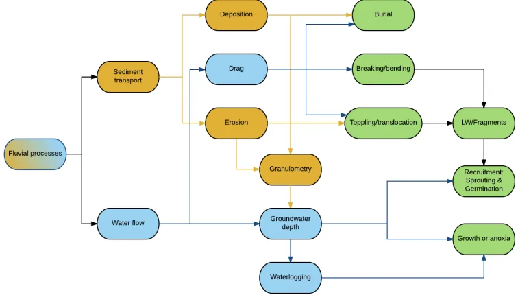
The hierarchy of fluvial processes that affect riparian vegetation (Figure 1-2) is partitioned into sediment transport and water flow, with sediment transport further divided into deposition and erosion and water flow further divided into drag and groundwater depth. Fluvial process feedbacks to vegetation occur at different temporal scales. Drag, erosion and deposition exert their disturbance pressure during floods, when plants can be buried by sediments, broken and bent by flow drag, or toppled and translocated by excessive erosion associated with drag pull (Bendix and Hupp, 2000; Steiger et al., 2005). On a longer time scale, the geomorphic action of floods builds the physical setting, providing the substrate and the hydration conditions for the riparian vegetation life cycle (Hupp and Osterkamp, 1996).

(26)

1.3 Salicaceae feedbacks to fluvial processes

Many studies concerned with vegetation-fluvial process interaction are not “Salicaceae specific”. However, many of these studies have been included in this review when they have a sufficient degree of generality to make their conclusions applicable to the Salicaceae.

1.3.1 Roots

Roots provide additional substrate cohesion thus increasing the shear load required to mobilize the substrate (Reubens et al., 2007). The shear load can cause failure of a single root either because of breakage or pullout (Coppin and Richards, 2007). Pullout resistance can be seen as a measure of root-soil friction and is a function of root length and diameter. For a single root it can be defined (Ennos, 1990) as:

!_" = $ & 2() Equation 1-1

where Fp is the pullout force per unit area (kPa), S is the shear strength of the soil (KPa), r is the radius of the root (m) and L is the length of the root (m). If the soil friction holding the root is greater than the root’s Fp, the root can also break before the tractive force Fp is reached. The force to break a root was defined by Pollen & Simon (2005) as:

!_* = +,-* Equation 1-2

where Fb is the breakage force per unit area (kPa), corresponding to root tensile strength, and a and b are species-specific coefficients estimated from field data (Figure 1-3). Figure 1-3 shows also how finer roots have higher tensile strength per unit area than coarser ones, therefore suggesting that a large number of fine roots have a better stabilization effect than fewer coarse roots with the same root area ratio.

Figure 1-3 Tensile strength per unit area calculated for three species of Salicaceae with Eq. 1. Data sources: (Pollen and Simon, 2005; Polvi et al., 2014; Simon et al., 2006)

(27)

27

caused by root tortuosity, which increases the root-soil friction. The breakage diameter threshold changes according to substrate type and substrate moisture and, as these two properties change with space and time, respectively (Konsoer et al., 2016; Pollen, 2007), breakage diameter is a dynamic attribute of roots. Increased substrate moisture results in lower root-substrate friction and thus a higher breakage diameter threshold (Pollen, 2007). Different substrate types exhibit different shear strength (term S in Equation 1-1 thus resulting in different friction values for a unit area of roots. Despite the variability, the diameter threshold seems to fall between 2.5 and 3.5 mm with breakage being the dominant failure process below the threshold and pull out above it.

1.3.1.1 Substrate cohesiveness

1.3.1.1.1 Bank stability

The effect of vegetation on bank stability can have deep impacts on the overall planform evolution of a river as vegetation is able to induce a change in river planform style from braiding to single thread / meandering (Gibling and Davies, 2012; Gran and Paola, 2001).

(28)

Table 1-1 Roots reinforcement estimated by RipRoot model for a bank 10 m long and a shear surface length of 1.15 m (Pollen and Simon, 2005)

Species Number of roots ∆S (kPa)

P. fremontii

200 0.41

400 0.82

600 1.23

800 1.65

1000 2.05

S. nigra

200 0.84

400 1.68

600 2.52

800 3.37

1000 4.2

(29)

29

Figure 1-4 Modelled Populus fremontii and Salix nigra increase in soil cohesion in relation to age. Data source: (Pollen-Bankhead and Simon, 2009).

1.3.1.1.2 Erosion of (in-channel) non-cohesive material

Studies on root enhancement of non-cohesive substrates have received far less attention than bank failure and erosion of cohesive substrates. With respect to bank failure, surface erosion of non-cohesive material does not occur along a preferential failure plane but it rather proceeds by gradual abduction of the substrate. Therefore, root cohesion approaches developed in relation to bank stability fail to capture non cohesive in-channel erosion mechanisms (Pasquale and Perona, 2014). Modelling of such mechanisms has been achieved by increasing the critical shear of the substrate (Bertoldi et al., 2014) or by reducing the eroded quantity by a percentage depending on vegetation cover (Van De Wiel et al., 2007). However, to our knowledge, there is no empirical evidence to support the parameterization of the two methods. Pasquale & Perona (2014) devised and tested a possible strategy for their quantification. The results from their field experiment with Salix cuttings revealed a tendency of reduced scour where vegetation was present and increased substrate cohesion in correspondence with root maximum volume. The increase in cohesion was computed to fall within an approximate range of 1.0-2.5 % (Pasquale and Perona, 2014). Such a low increase can be explained by the young age of the cuttings that had not developed extended root systems and by the limited dataset available for analysis.

1.3.2 Canopy and stem

When partly or fully submerged, plant aerial structures affect the flow field by deflecting the water and dissipating energy. The effects include an increase of flow velocity around the plants, while velocity is reduced inside vegetated stands (Schnauder and Moggridge, 2009). These processes are particularly relevant when sediment transport occurs.

1.3.2.1 Flow resistance

(30)

resistance varies temporally and spatially. The resistance offered by a single vegetation element to flowing water can be described by the drag force (FD) Equation 1-3:

!. = /₀12.3"40 Equation 1-3

where ρ is the water density, AP is the frontal projected area of vegetation exposed to the flow, U is the mean flow velocity and CD is the drag coefficient, a lumped coefficient that includes friction and form drag. For rigid, tree-shaped individuals with emergent canopies, Equation 1-3 represents a sufficient approximation but for totally or partially submerged flexible plants, such as Salicaceae shrubs, this formulation is difficult to apply (Aberle and Järvelä, 2013). Nevertheless, from a theoretical viewpoint Equation 1-3 is correct and is reported here because it allows a complete consideration of all the key elements of vegetation flow resistance. When flow velocity is sufficiently high, flexible plants streamline in the direction of the flow, thus reducing AP and CD (Fathi-Maghadam and Kouwen, 1997; Gosselin and De Langre, 2011; Weissteiner et al., 2015). Streamlining is exacerbated by the presence of leaves (Freeman et al., 2000; Järvelä, 2002a). Therefore, for deciduous species such as those of the Salicaceae, resistance changes seasonally. AP also varies with water depth. Under partial submergence, as water depth increases more of the plant-area is exposed to the flow, thus increasing flow resistance (Fathi-Maghadam and Kouwen, 1997; Manners et al., 2013). Conversely, under fully submerged conditions, resistance increases linearly with depth until a certain level beyond which resistance decreases until it reaches an asymptotic constant (Manners et al., 2013; Wu et al., 1999). The degree of submersion also has a strong influence on the velocity profile (see section 1.3.2.2), which in turn determines the mean velocity U (Equation 1-3). In the relationship between flow and flexible vegetation, flow resistance is thus a dynamic attribute whose estimation is complicated by continuous interaction between vegetation and flow properties that determines flow resistance.

At the patch scale, flow resistance depends on the longitudinal and lateral distance among individuals (i.e. stem density), with the resistance positively correlated with decreasing distances between stems (Righetti, 2008). In a recent review Aberle & Järvelä (2013) noted how vegetation density and reconfiguration are the main features to be considered in flow resistance equations and that such equations should be based on species specific parameters such as the one developed by Västilä & Järvelä, (2014). This latter method is particularly suited to practical applications because vegetation parameterization relies on measureable plant properties (Antonarakis et al., 2010, 2009, Jalonen et al., 2015, 2013), considers plant reconfiguration, and accounts for different flow depths (Aberle and Järvelä, 2013; Västilä and Järvelä, 2014).

1.3.2.2 Flow deflection

The flow resistance provided by vegetation causes flow field velocity vectors to deviate from their original trajectories. For single, tree-like plants whose canopy is emergent, the flow deflection effect is similar to that of a bridge pier, generating horseshoe vortices on the upstream side of the stem (Unger and Hager, 2007) and creating wakes and local flow acceleration on the downstream side of the stem (Ahmed and Rajaratnam, 1998).

(31)

31

Figure 1-5 Effects of a finite width patch on the flow field horizontal dimension. Adapted from (Nepf, 2012)

In the second case of patches with a circular shape of diameter DG (Figure 1-6), vegetation drag causes stem scale turbulence that decreases the approaching velocity U0 to a lower velocity U1 downstream from the patch (Nepf, 2012). Flow interactions and patch wake characteristics depend on stem densities that can be expressed also as a void fraction (Φ) calculated as:

Φ = Nc (D/DG) 2 _{Equation 1-4}

where Nc is the number of stems, DG is the patch diameter and D is the diameter of the stems (Nicolle and Eames, 2011). For Φ < 0.05 the stems behave as isolated entities; when 0.05 < Φ < 0.15 a shear layer occurs at the streamwise sides of the patch; and for Φ > 0.15 the patch acts as a solid body of similar diameter. Because the flow downstream from the patch is slower than the flow in the open channel, when the shear layer forms (i.e. 0.05 < Φ < 0.15) flow “bleeding” (sensu Schnauder & Moggridge 2009) through the patch interferes with the shear layer and delays the formation of patch-scale Von Karman vortices (VK) (See Nepf 2012b for an in-depth explanation of the mathematical aspects).

Figure 1-6 Effects of a circular patch on the flow field horizontal dimension. Adapted from (Nepf, 2012)

(32)

is reduced (Figure 1-7 B). In the case of submerged vegetation, flow velocity above the vegetated patch displays a logarithmic profile (Figure 1-7 A).

Figure 1-7 Effects on the flow field vertical distribution of a submerged (A) and partially submerged (B) patch. Adapted from (Baptist et al., 2009) and (Nepf and Vivoni, 2000)

1.3.2.3 Effects of flow alteration on sediment transport, erosion and deposition

For a single stemmed plant, the horseshoe vortex on the upstream side of the stem enhances local erosion around the stem’s upstream and streamwise sides (Unger and Hager, 2007). A similar situation occurs around densely vegetated patches, as the blockage by the plants resembles that of a single solid bluff body (Nicolle and Eames, 2011; Zong and Nepf, 2010).

(33)

33

Figure 1-8 Scour and deposition measured in a flume experiment, for a channel side and a centre bar with flexible objects simulating flexible submerged vegetation. Scour was measured upstream and on the sides of the bars, deposition was measured downstream from the bars. Plant density is the ratio of the projected area of the flexible objects and the area of each bar. In the charts, a plant density of 1 indicates a solid, non-flexible object with the same bar area and object height as that of the flexible objects. Data source: Chen, Kuo & Yen 2012b

1.4 Fluvial process feedbacks to Salicaceae

Fluvial processes influence Salicaceae by exerting stresses or disturbances or regulating limiting factors. These three types of influence operate on different time scales. Limiting factors are extremely unlikely to change and therefore are a persistent constraint on plants (e.g. light, nutrients or water). A stressor is an external factor that reduces dry matter production of one or more plant organs during a more limited period of time (Grime, 2002) such as the occurrence of a drought period. A disturbance occurs over a very short period of time, damaging or disrupting an ecosystem and changing its physical condition and its population structure and communities (Pickett & White 1985, p. 7). In the riparian context, disturbances are usually related to the occurrence of floods.

The following sections mainly consider stress and disturbance as impacts on vegetation. Biological responses encompass both resistance and recovery mechanisms where resistance is the set of traits and properties that allow an individual plant to endure a stress or a disturbance while recovery mechanisms are the set of traits and properties that allow plant communities to regain their vigour after a disruptive event, thus forming part of the concept of ecological resilience.

1.4.1 Water flow

1.4.1.1 Groundwater depth

(34)

et al., 1999; Polzin and Rood, 2006). Since propagules are often deposited by declining flood waters, the position of the water table is usually governed by the rate of decline of the falling limb of the flood hydrograph and substrate properties (Mahoney and Rood, 1998). On gravel bars, moisture can be retained by the combined presence of coarse-gravel standing on a finer sediment matrix. The superficial gravel acts as a mulch thus reducing evaporation and maintaining high moisture for weeks even without alluvial or meteoric water inputs (Meier and Hauer, 2010).

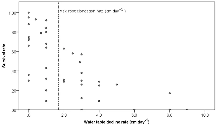
Many researchers have investigated experimentally the rate of root growth of seedlings and cuttings subjected to different combinations of substrate granulometry and rates of water table decline (Table 1-5). Decline rates greater than 2.5 to 3 cm day-1 appear to be lethal for the seedlings of most of the Salicaceae (Mahoney and Rood, 1998; Stella et al., 2010) regardless of substrate type. During controlled experiments, the highest survival rates have been observed for water table decline rates of less than 2 cm day-1 (Figure 1-9) and maximum root daily elongation rates of 1.5 and 1.7 cm day-1 have been observed for seedlings and cuttings, respectively (Table 1-5). However, the extremes reported in Table 1-5 should be considered with caution because in natural settings, shallow rooted plants are unlikely to survive the most extreme conditions tested in these experiments (Amlin and Rood, 2002; González et al., 2010).

Figure 1-9 Survival of seed-recruited seedlings under different water table decline rates (Data source: Table 1-5)

DGW and granulometry are also of utmost importance for the sprouting of pieces of deposited large wood (LW, > 1 m long and 10 cm diameter) and smaller wood fragments (Francis et al., 2006; Francis and Gurnell, 2006). However, differences in the sampling methods employed in published studies prevent precise quantification of the most suitable quantitative ranges for sprouting (Table 1-7). In general terms, successful sprouting occurs at locations low enough to guarantee sufficient moisture but elevated enough to provide shelter from subsequent floods that would otherwise remobilize the deposited wood. Suitable shelter can also be provided at lower elevations in the lee of obstructions such as islands (Moggridge and Gurnell, 2009).

(35)

35

Drought stress leads to a reduction of the plant water potential with consequent stomatal closure and impaired transpiration (Van Splunder et al., 1996). For the Salicaceae, if the plant water potential decreases below approximately -0.7/-1.7 MPa (Horton et al., 2001; Tyree et al., 1994), xylem cavitation can occur, followed in the most severe cases by senescence and abscission of branches (Rood et al., 2000). Other responses are the reduction in the shoot-to-root ratio, reduced transpiration rates, more efficient use of available water, and a reduction of leaf area (Stella and Battles, 2010; Van Splunder et al., 1996).

For P. deltoides subsp. Monilifera (Aiton) Eck, sustained GWD declines that are less than or equal to 0.5 – 0.6 m have little or no effect on crown vigour of adult individuals while declines greater than 1 - 1.5 m cause considerable crown dieback, reduced growth and branch abscission (Cooper et al., 2003; Scott et al., 1999). In arid climates, the response time to such GWD decline is shorter than a week (Cooper et al., 2003) and if the stress persists to the following growing season, the vast majority of individuals are likely to die (Scott et al. 1999; Scott, Lines & Auble 2000; Shafroth, Stromberg & Patten 2000). The decrease in annual growth performance in response to GWD lowering was also observed for Populus fremontii Watson and Salix exigua Nutt. (Hultine et al., 2010). In the first growing season following GWD decline, cottonwood and willow exhibited a radial growth decrease of 22-30% and 32-40%, respectively. Growth rates returned to normal in the growing season after the GWD was reset to the natural range (Hultine et al., 2010).

Fluctuations in GWD are part of natural riparian system functioning and so may not result in adverse consequences for plants and can even promote root elongation in the soil pores vacated by the falling water level (Naumburg et al., 2005). However, the amplitude of such fluctuations appears to be a habitat factor that constrains Salicaceae populations within loosely defined fluctuation boundaries. Along the San Pedro River, Arizona, Lite and Stromberg, (2005) observed that Populus fremontii and Salix goddingii abundances declined where annual GWD fluctuations exceeded 0.8 m and 0.5 m, respectively, although the absolute value of GWD appears to be less important than the decline rate. Drought effects on Salicaceae ultimately depend on the counterbalance between root elongation and the rate of GWD decline, since root depth is a plastic trait that can change according to water table fluctuations. In a two-year field experiment with S. alba and S. viminalis cuttings, Pasquale et al. (2014) observed that the depth at which roots achieve maximum density could change during the growing season. Such behaviour is formalized by Equation 1-5 (Pasquale et al., 2012) where Zr and Zw are the mode of maximum root density elevation and water table elevation (above sea level), respectively, Zs is the mean surface elevation during the growing season and η is a scaling parameter corresponding to the site and species tested in Pasquale et al. (2012).

Z_>= ηZ@+ ZB

1 + η Equation 1-5

(36)

(37)

37

Table 1-2 Maximum groundwater depth for survival of Populus and Salix species (expanded from Lite and Stromberg, 2005)

Species

Groundwater maximum depth (m)

Location Reference

Sa p lin g s u rv iv a l P. fremontii 2.91

Bill William River, AZ where

water table had regular interannual fluctuations

Shafroth et al., 2000 S. gooddingii

P. fremontii

0.82 and 3.14

Bill William River, AZ where

water table were relatively shallow and stable

Shafroth et al., 2000 S. gooddingii

P. fremontii 2.93 Bill William River, AZ Shafroth et al., 1998 a

S. gooddingii 2.02 Bill William River, AZ Shafroth et al., 1998 a

P. fremontii

2 San Pedro River, AZ Stromberg et al., 1996

S. gooddingii

P. fremontii 1 Hassayampa River, AZ Stromberg et al., 1991

Ad u lt su rv iv a l P. fremontii

2.5 – 3 Hassayampa River, AZ

Horton et al., 2001 a

and

Horton et al., 2001 a S. gooddingii

P. fremontii 2.6 Hassayampa River, AZ Stromberg et al., 1991

P. fremontii 5.1 San Pedro River, AZ Stromberg et al., 1996

S. gooddingii 3.2 San Pedro River, AZ Stromberg et al., 1996

P. fremontii

1.5 – 3 Bill Williams River, AZ Busch and Smith, 1995

S. gooddingii P. fremontii

3 – 4.5 Lower Colorado River, AZ Busch and Smith, 1995

S. gooddingii P. fremontii

1.3 – 3.5 San Pedro River, AZ Lite and Stromberg, ₂₀₀₅ S. gooddingii

a_{Studies designed to detect threshold values, other values are for observed ranges of occurrence.}

GWD and related river discharge also regulate Salicaceae annual growth performances since GWD is strongly dependent on flow stage (Cooper et al., 1999) and annual growth is linearly correlated to streamflow (Stromberg and Patten, 1996; Willms et al., 1998) with growth increasing when annual flows are above the long-term annual mean (Stromberg and Patten, 1996). Within the growing season in glacial fed reaches, late winter and spring flow stages appear to be better growth predictors than late spring and early summer ones, probably because the water table is replenished by peak flows occurring at the end of the winter (Willms et al., 1998).