A fuzzy-random programming for integrated closed-loop logistics network design by using priority-based genetic algorithm Pages 139-154 Download PDF

(1)

* Corresponding author. +98 21 88192570

International Journal of Industrial Engineering Computations 4 (2013) 139–154

Contents lists available at GrowingScience

International Journal of Industrial Engineering Computations

homepage: www.GrowingScience.com/ijiec

A fuzzy-random programming for integrated closed-loop logistics network design by using priority-based genetic algorithm

Emad Roghanian and Keyvan Kamandanipour*

Department of industrial engineering, K.N Toosi University of Technology, Tehran, Iran

A R T I C L E I N F O A B S T R A C T

Article history: Received 18 July 2012 Received in revised format 14 August 2012

Accepted September 10 2012 Available online

15 September 2012

Recovery of used products has steadily become interesting issue for research due to economic reasons and growing environmental or legislative concern. This paper presents a closed-loop logistics network design based on reverse logistics models. A mixed integer linear programming model is implemented to integrate logistics network design in order to prevent the sub-optimality caused by the separate design of the forward and reverse networks. The study presents a single product and multi-stage logistics network problem for the new and return products not only to determine subsets of logistics centers to be opened, but also to determine transportation strategy, which satisfies demand imposed by facilities and minimizes fixed opening and total shipping costs. Since the deterministic estimation of some parameters such as demand and rate of return of used products in closed loop logistics models is impractical, an uncertain programming is proposed. In this case, we assume there are several economic conditions with predefined probabilities calculated from historical data. Then by means of expert's opinion, a fuzzy variable is offered as customer's demand under each economic condition. In addition, demand and rate of return of products for each customer zone is presented by fuzzy-random variables, similarly. Therefore, a fuzzy-random programming is used and a priority-based genetic algorithm is proposed to solve large-scale problems.

Integrated logistics network Closed-loop logistics Genetic algorithm (GA) Priority-based encoding Fuzzy-random programming

1. Introduction and literature review

1.1. Closed loop logistics network design

(2)

form a continuous process to treat return-product items until they are properly recovered or disposed. These activities include collection, cleaning, disassembly, test and sorting, storage, transport, and recovery operations. The latter can also be represented as one or a combination of several main recovery options, like reuse, repair, refurbishing, remanufacturing, cannibalization and recycling (Lu & Bostel, 2007). Reverse logistics is getting increasingly important as a profitable and sustainable business strategy. There are a number of situations for products to be placed in a reverse flow. Normally, return flows are classified into commercial, warranty and end-of-use returns, reusable container returns, etc. (Du & Evans, 2008). Implementation of reverse logistics especially in product returns not only saves inventory carrying, transportation, and waste disposal costs due to returned products, but also it improves customer loyalty and futures sales (Ko & Evans, 2007). Reverse logistics systems are more complex than forward logistics systems, which stems from a high degree of uncertainty due to the quantity and quality of the products (Kara & Rugrungruang, 2007). Reverse logistics has attracted much attention recently due to growing environmental or legislative concerns and economic opportunities for cost savings or revenues from returned products.

Barros et al. (1998) proposed a mixed integer linear programming (MILP) model based on a multi-level capacitated warehouse location problem for sand and proposed a heuristic method to solve the resulted model. The model determined the optimal number, capacities, and locations of the depots and cleaning facilities. Kirkke et al. (1998) presented a MILP model based on a multi-level uncapacitated warehouse location model. They presented a case study, which deals with a reverse logistics network for the returns, processing, and recovery of discarded copiers. The model was used to determine the locations and capacities of the recovery facilities as well as the transportation links connecting various locations. Jayaraman et al. (1999) proposed another MILP model to determine optimal numbers and locations of distribution/remanufacturing facilities for electronic equipment.

Jayaraman et al. (2003) developed the other MILP model and solution procedure for a reverse distribution problem focused on the strategic level. The model determines whether each remanufacturing facility is open considering the product return flow. Min et al. (2005) proposed a Lagrangian relaxation heuristics to design the multi-commodity, multi-echelon reverse logistics network. Kim et al. (2006) proposed a general framework for remanufacturing environment and a mathematical model to maximize the total cost saving. The model determines the quantity of products/parts processed in the remanufacturing facilities/subcontractors and the amount of parts purchased from the external suppliers while maximizing the total remanufacturing cost saving. Min et al. (2006) proposed a nonlinear mixed integer programming model and a genetic algorithm, which could solve the reverse logistics problem involving product returns. Their study proposed a mathematical model and GA, which aims to provide a minimum-cost solution for the reverse logistics network design problem involving product returns.

(3)

1.2. Hybrid programming

Uncertainty is one of the main characteristics of reverse logistics network problem, which further increases the complexity of the problem. The degree of uncertainty in terms of the capacities, demands and quantity of products exists in reverse logistics parameters. An important issue, when manufacturing centers' demands as well as recycling centers' demand are random variables in reverse logistics' network design problem, is to find the network strategy, which could achieve the objective of minimization of total shipping cost and fixed opening expenditures of the disassembly and the processing centers. This paper proposes a probabilistic MILP model for the design of a reverse logistics network. This probabilistic model is first converted into an equivalent deterministic model.

There are some mathematical programming which deals with the theory and methods for the solution of conditional extremum problems under incomplete information about the random parameters called “stochastic programming”. Fuzziness, on the other hand, is associated with the unsharp boundaries of the parameters of the model, and can be traced to sources of uncertainty such as modeling choices, parameter choices, application of expertise, boundary conditions, and lack of knowledge. Thus, randomness is more an instrument of a normative analysis, which focuses on the future and fuzziness and it is more a tool for a descriptive analysis to reflect the past and its implications. Clearly, randomness and fuzziness are complementary. One important aspect of this relationship is the fuzzy-random variable (FRV), which is a measurable function from a probability space to the set of fuzzy variables (Shapiro, 2009). A simple type of programming, which simultaneously deals with random and fuzzy nature of the uncertain models is called “hybrid programming” and the special type of this programming, which solves the resulted model including FRVs is “fuzzy-random programming”. Unfortunately, the SCN design problem is subject to many sources of uncertainty besides random uncertainty and fuzzy uncertainty (Huang, 2006) and in many practical decision-making issues, we deal with a hybrid uncertain environment. To deal with twofold uncertainties, fuzzy random variable was proposed by Kwakernaak (1978) to depict the phenomena in which fuzziness and randomness appear, simultaneously. As mentioned earlier, in SCN design problem, uncertainty in some parameters such as demand of customer zones and rate of return of used products from customers is reasonable. Although there are some approaches to solve models with hybrid and particularly fuzzy random parameters (such as Liu (2002a, 2002b) and Liu and Liu(2003) ), there are only a few researches about SCN design with hybrid parameters. This point is more critical for integrated logistics network designs. Nonetheless there are some papers in facility location allocation in hybrid environment, for example Wen and Imamura (2008), Wen and Kang (2011). In this paper, we develop an integrated logistics network design model with fuzzy-random demands and rate of returned products.

1.3. Priority-based genetic algorithm

(4)

n be the number of sources and depots, respectively, then the dimension of matrix will be m*n.

Although representation is straightforward, this approach requires special crossover and mutation operators for obtaining feasible solutions.

Gen and Cheng (2000) introduced spanning tree GA (st-GA) for solving network problems. They used Prüfer number representation for solving transportation problems and developed feasibility criteria for Prüfer number to be decoded into a spanning tree. Syarif et al. (2002) proposed spanning tree-based genetic algorithm by using prüfer's number representation for solving a single product, three-stage supply chain network (SCN) problem. Xu et al. (2008) applied spanning tree-based genetic algorithm (st-GA) by the Prüfer number representation to locate the SCN to meet the demand imposed by customers with minimum total cost and maximum customer services for a multi objective SCN design problem. Although Prüfer number developed to encode of spanning trees, has been successfully applied to transportation problems, it needs some modifications to reach feasible solutions after classical genetic operators.

In this study, to escape from these repair mechanisms in the search process of GA, we concentrate on the priority-based encoding method. Gen et al. (2006) used priority-based encoding for a single-product, two-stage transportation problem. Altiparmak et al. (2006) applied priority-based representation to a single- product, single-source, and three-stage SCN problem, Altiparmak et al. (2009) proposed this encoding to a single-source, multi-product, multi-stage SCN problem. Lee et al. (2009) proposed a hybrid genetic algorithm with priority-based encoding method.

In this paper, we propose single-product, multi-stage integrated logistics network problem, which consider the minimizing of total shipping cost and fixed opening costs of the hybrid production/recovery centers, hybrid distribution/collection and disposal centers. In fact, this type of network design problem belongs to the class of NP-hard problems, so that priority based genetic algorithm could be presented to solve large scale problems. Finally, we apply the proposed model for an example problem and present some numerical results.

The remainder of this paper is organized as follows: The problem definition and mathematical model of integrated closed-loop logistics network design with hybrid parameters are introduced in section 2. Then in section 3, solution approach including priority-based genetic algorithm and fuzzy-random programming is discussed. Illustrative numerical examples and the results for evaluation are given in section 4. Finally, concluding remarks and future researches are outlined in section 5.

2. Problem definition and formulation

2.1 Problem definition

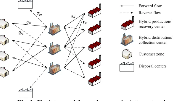
There are many modeling approach for supply chain network design of reverse and forward logistics flows. The logistics network discussed in this paper is an integrated logistics one, which models forwards and reverses flows. The mentioned integrated logistics network, which is based on Pishvaee et al. (2009), is a single product, single period, multi-stage logistics network. There are four kinds of logistics node including customer zones, production, recovery, distribution, collection centers and disposal centers. As stated by Pishvaee et al. (2009) in such an integrated logistics network, hybrid logistics facilities offer more advantages compared with separate distribution or collection centers. The advantages include both cost savings and pollution reduction as results of sharing material handling equipment and infrastructures (Shen, 2007).

(5)

experiments is difficult. Instead, expert opinion is used to provide the estimations. Unfortunately sometimes using fuzzy variables cannot overcome on this kind of uncertainty, properly. Lack of attention to hidden aspect of randomness in these parameters could be a reason of this problem. In this case, fuzziness and randomness of the customers’ demands are mixed up. The primary assumption is that there are several economic conditions with predefined probabilities, which can be calculated from historical data. Then, by means of expert opinions, a fuzzy variable is offered as demand of the customer under each economic condition. So the demand of each customer zone is presented by a fuzzy-random variable. Similarly, another fuzzy-random variable is offered for rate of return of products. As shown in Fig.1, in the forward flow in a pull system, products are shipped from hybrid production/recovery centers through hybrid distribution/collection centers to customer zones to meet customers’ demand. In the reverse flow through a push system, returned products are collected by distribution-collection centers and after inspection the recoverable products are shipped to production/recovery centers, and scrapped products are shipped to disposal centers.

After the processes of recovery, the recovered products are used as new products in forward flows. A predefined fuzzy-random rate of demand and a predefined fuzzy-random percentage of demand of each customer zone are assumed as rate of returned products and a predefined value is determined as an average disposal rate. High quality returned products are more capable for recovery processes and low quality ones should be disposed in a safe process.

Forward flow Reverse flow

Hybrid production/ recovery center

Hybrid distribution/ collection center

Customer zone

Disposal centers

Ujk

Xij

Qkj

Vji

Tjm

Fig. 1. The integrated forward-reverse logistics network 2.2 Mathematical formulation

Based on mentioned assumptions, the main issues to be addressed by this paper are to select the location and to determine the number of hybrid distribution/collection, hybrid production/recovery and disposal centers and to quantify the products shipped among logistics facilities. The notations used for the considered problem are listed below:

Parameters:

I Set of potential production/recovery center locations i ∈ I

J Set of potential hybrid distribution/collection center locations j ∈ J K Fixed locations of customer zones k ∈ K

M Set of potential disposal center locations m ∈ M

k

ξ _{Fuzzy-random demand of customer zone}_k

k

η _{Fuzzy-random rate of return of used products from customer zone}_k s Average disposal fraction

fi Fixed cost of opening hybrid distribution/collection center j

(6)

hm Shipping cost per unit of products from production/recovery center

i to hybrid

distribution/collection center j

cij Shipping cost per unit of products from hybrid distribution/collection center j to customer zone k

ajk Shipping cost per unit of returned products from customer zone _{distribution/collection center} k to hybrid

j

bkj Shipping cost per unit of recoverable products from hybrid distribution/collection center _{production/recovery center} j to

i

eji Shipping cost per unit of scrapped products from hybrid distribution/collection center

j to

disposal center m

pjm Manufacturing/recovery cost per unit of product at production/recovery center i

cwi Capacity of production for production/recovery center i

cyj Capacity of handling products in forward flow at hybrid distribution/collection center j

czm Capacity of handling scrapped products at disposal center m

cyrj Capacity of handling returned products in reverse flow at hybrid distribution/collection center j

cwri Capacity of recovery for production/recovery center i

Variables:

Xij

Quantity of products shipped from production/recovery center i to hybrid distribution/collection

center j

Ujk Quantity of products shipped from hybrid distribution/collection center j to customer zone k

Qkj Quantity of returned products shipped from customer zone

k to hybrid distribution/collection

center j

Vji Quantity of recoverable products shipped from hybrid distribution/collection center

j to

production/recovery center i

Tjm Quantity of scrapped products shipped from hybrid distribution/collection center

j to disposal

center m

1 if a production/recovery center is opened at location

0 otherwise

i

i, W = ⎨⎧

⎩

1 if a hybrid distributioncollection center is opened at location ,

0 otherwise

j

j Y = ⎨⎧

⎩

1 if a disposal center is opened at location ,

0 otherwise

i

m W = ⎨⎧

⎩

The problem can be formulated as follow:

min _i _i _j _j _m _m _ij _ij _jk _jk _kj _kj _ji _ji _{jm jm}

i I i I m M i I j J i I j J k K j J j J i I j J m M

f W g Y h Z c X a U b Q e V p T

∈ ∈ ∈ ∈ ∈ ∈ ∈ ∈ ∈ ∈ ∈ ∈ ∈

+ + + + + + +

∑

∑∑

∑ ∑

(1)

subject to

jk k

j J

U ξ k K

∈

≥ ∀ ∈

∑

(2)

kj k k j J

Q η ξ k K

∈

≥ ∀ ∈

∑

(3)

ij jk

j J k K

X U 0 j J

∈ ∈

− = ∀ ∈

∑

(4)

ji kj

i I k K

V ( 1 s ) Q 0 j J

∈ ∈

− − = ∀ ∈

∑

(5)

jm kj

m M k K

T s Q 0 j J

∈ ∈

− = ∀ ∈

∑

(6)

ji ij

j J j J

V X 0 i I

∈ ∈

− ≤ ∀ ∈

(7)

ji i i j J

X cw W i I

∈

≤ ∀ ∈

∑

(8)

ij j j

i I

X cy Y j J

∈

≤ ∀ ∈

∑

(9)

kj j j

k K

Q cyr Y j J

∈

≤ ∀ ∈

∑

(10)

ji i i

i I

V cwrW i I

∈

≤ ∀ ∈

∑

(11)

jm m m

j J

T cz Z m M

∈

≤ ∀ ∈

∑

(12)

{ }

i j m

W ,Y ,Z ∈ 0,1 ∀ ∈ ∀ ∈ ∀ ∈i I , j J , m M (13)

ij jk kj ji jm

X ,U ,Q ,V ,T ≥0 ∀ ∈ ∀ ∈ ∀ ∈i I , j J , m M , k∀ ∈K (14)

where:

(15)

11 12 13 14 1

k 21 22 23 24 2

31 32 33 34 3

(d ,d , d ,d ) with probability p (d ,d , d , d ) with probability p (d , d , d ,d ) with probability p ⎧

⎪ ξ = ⎨ ⎪ ⎩

(16)

11 12 13 14 1

k 21 22 23 24 2

31 32 33 34 3

(r , r , r , r ) with probability p (r , r , r , r ) with probability p (r , r , r , r ) with probability p ⎧

⎪ η = ⎨ ⎪ ⎩

The objective function (1) minimizes the total cost of the forward and reverse logistics. It consists of the logistics shipping cost and fixed opening cost of the facilities. Constraints (2) and (3) ensure that the demands of all customers are satisfied and the returned products from all customers are collected. Constrains (4)-(7) balance flows between production/recovery and distribution/collection centers in forward and reverse flows. Constrains (8)-(12) explain about capacity of each facilities. Constraint (13) imposes the binary restriction on the decision variables Wi, Yj, Zm and constraint (14) imposes the non-negativity restriction on the other decision variables.

3.Solution approach

We propose priority-based GA to solve the deterministic integrated closed-loop logistics network design model. Then it is developed for solving uncertain model with fuzzy-random parameters.

3.1. Priority-based genetic algorithm

(8)

Algorithm 1: Priority-based decoding: Inputs:

K: set of sources

J: set of depots

b: demand on depot j, ∀jϵ J a : capacity of source k, ∀ kϵK

c : transportation cost of one unit of product from source k to depot j, ∀ kϵK, ∀jϵ J

+ : chromosome, ∀ kϵK, ∀jϵ J

Outputs:

: the amount of product shipped from source k to depot j

While ∑ ≥ 0

Step 1: = 0 , ∀ kϵK, ∀jϵ J

Step 2: select a node based on l =arg max {v t , tϵ|k| + |j|}, ∀ kϵK, ∀jϵ J Step 3: if lϵK then a source is selected k∗= l ,

j∗₌_{arg min {}_{c | v j ≠ 0, j}_ϵ_J}_{, Select a depot with minimum cost}

else ∗= l a depot is selected

k∗₌_{arg min {}_{c | v j ≠ 0, k}_ϵ_K}_{, Select a source with minimum cost}

Step 4: ∗ ∗ =min{ ∗, ∗}

Update demands and capacities

∗= ∗− ∗ ∗ ∗ = ∗− ∗ ∗

Step 5: if ∗ = 0thenv ∗ = 0 if ∗ = 0thenv ∗ = 0

Step 6: if + = 0, ∀jϵ Jthen output and calculate transportation cost, elsereturn step 1

End

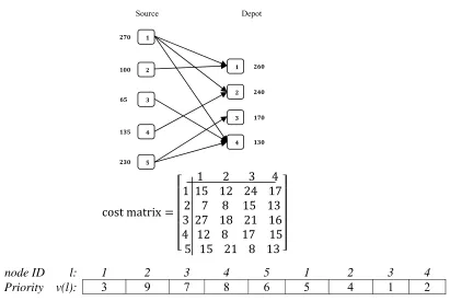
Fig. 2 represents a transportation tree with 5 sources and 4 depots, its cost matrix and priority based encoding. Table 1 gives trace table of the decoding procedure to obtain transportation tree in Fig. 2

cost matrix =

1 2 3 4 1 15 12 24 17

2 7 8 15 13 3 27 18 21 16 4 12 8 17 15 5 15 21 8 13

Fig. 2. A sample of transportation tree and its encoding

4 3

2 1

5 4

3 2

1 node ID l:

2 1

4 5

6 8

7 9

3

Priority v(l):

(9)

Table 1

Trace table of decoding procedure.

Iteration v(k+j) A b k j

0 [3 9 7 8 6 |5 4 1 2] (270,100,65,135,230) (260,240,170,130) 2 1 100

1 [3 0 7 8 6 |5 4 1 2] ( 270, 0, 65,135,230) (160,240,170,130) 4 2 135

2 [3 0 7 0 6 |5 4 1 2] ( 270, 0,65,0,230) (160,105,170,130) 3 4 65

3 [3 0 0 0 6 |5 4 1 2] (270,0,0,0,230) (160,105,170,65) 5 3 170

4 [3 0 0 0 0 |5 4 1 2] (270,0,0, 0,60) (160,105,0,65 ) 1 1 160

5 [3 0 0 0 0 |0 4 1 2] (110,0,0, 0,60) ( 0,105,0,65) 1 2 105

6 [3 0 0 0 0 |0 0 1 2] (5,0,0,0,60) (0,0,0,65) 1 4 5

7 [0 0 0 0 0 |0 0 1 2] (0,0,0,0,60) (0,0,0,60) 5 4 60

8 [0 0 0 0 0 |0 0 1 0] (0,0,0,0,0) (0,0,0,0)

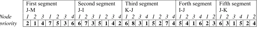
For the proposed problem of this paper, we use a chromosome consists of five segments, in which each one is associated with one echelon of the integrated closed-loop logistics network. We use segment J-M

to represent the transportation pattern from hybrid distribution/collection centers to disposal centers. Segment J-I is used to represent the transportation pattern from hybrid distribution/collection centers to

hybrid production/recovery centers. Segment K-J represents the transportation pattern from customer zones to hybrid distribution/collection centers. Segment I-J shows the transportation pattern from hybrid production/recovery centers to hybrid distribution/collection centers, segment determines J-K the transportation pattern from hybrid distribution/collection centers to customer zones (see Fig. 3). The chromosome of integrated closed-loop logistics network is decoded on a special sequence.

Fifth segment J-K Forth segment I-J Third segment K-J Second segment J-I First segment J-M 2 1 4 3 2 1 2 1 4 3 2 1 4 3 2 1 4 3 2 1 4 3 2 1 3 2 1 4 3 2 1 3 2 1 Node 4 2 5 1 3 6 3 2 6 1 4 5 4 7 2 5 1 3 8 6 2 4 1 5 3 7 6 6 3 5 7 4 1 2 priority

Fig. 3. An illustration of integrated closed-loop logistics network model chromosome.

The decoding algorithm of an integrated closed-loop logistics network chromosome is presented in Algorithm 2.

Algorithm 2: Integrated closed-loop logistics network decoding algorithm Inputs: ξk ،ηk ،_S،_f_i،_g_j،_h_m،_c_ij،_a_jk،_b_kj،_e_ji،_cw_i،_cy_j،_cz_m،_cyr_j.

Outputs: Xij،Ujk،Qkj،Vji،Tjm،Wi،Yj،Zm.

Step 1: calculate Ujk, Yj , ∀ , using Algorithm 1,

Step 2: calculate Xij , Wi ,∀ , using Algorithm 1,

Step 3: calculate Qkj , ∀ , using Algorithm 1,

Step 4: calculate Vji , ∀ , using Algorithm 1,

Step 5: calculate Tjm, Zm , ∀ , using Algorithm 1.

The proposed GA solution procedure used four genetic operators described below.

3.1.1. Parent selection operator

(10)

3.1.2. Crossover operator

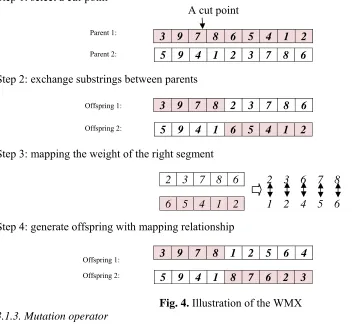
The crossover operator generates new offspring by combining information contained in the chromosomes of the parents so that new chromosomes will have the best parts of the parent’s chromosomes. The crossover is performed to explore new solution space and crossover operator corresponds to exchanging parts of strings between selected parents. Several crossover operators have been proposed for permutation representation, such as partially mapping crossover (PMX), order crossover (OX), position-based crossover (PX), cycle crossover (CX), weight mapping crossover (WMX), Heuristic crossover etc. (Lee et al., 2009). In this paper, we have used weight mapping crossover (WMX) operator, which is one-cut point crossover for permutation representation. As one point crossover, two chromosomes (parents) chooses a random cut-point and generates the offspring using segment of own parent to the left of the cut-point, then remapping the right segment based on the weight of other parent of right segment (Fig. 4).

Step 1: select a cut-point A cut point

Step 2: exchange substrings between parents

Step 3: mapping the weight of the right segment

Step 4: generate offspring with mapping relationship

Fig. 4. Illustration of the WMX 3.1.3. Mutation operator

After recombination, some children undergo mutation, similar to crossover; mutation is executed to prevent the premature convergence and explores new solution space. However, unlike crossover, mutation is usually performed by modifying gene within a chromosome. In this study, we have used insert mutation where a digit is randomly selected and it is inserted a randomly selected new position in chromosome. Fig. 5 represents insert mutation.

Select a gene at random

Insert it in a random position

Fig. 5. Illustration of the insert mutation

(11)

3.1.4. Evaluation operator

The evaluation aims to associate each individual with a fitness value so that it can reflect the goodness of fit for an individual. The evaluation process is intended to compare one individual with other individuals in the population. The choice of fitness function is also very critical because it has to accurately measure the desirability of the features described by the chromosome. The function should be computationally efficient since it is used many times to evaluate each solution (Gen & Cheng, 2000). In this study, the objective function has been taken as fitness function.

3.3. Fuzzy-random programming

In this section, we shall recall some basic concepts and results on random fuzzy variable. These results are crucial for the remainder of this paper. An interested reader may consult Liu (2009) where important properties of random fuzzy variables are recorded.

Let Θ be a nonempty set, (Θ) the power set of Θ, and Pos a possibility measure. Then the triplet (Θ,P(Θ),Pos) is called a possibility space. A fuzzy variable ξ is defined as a function from a possibility

space (ξ,P(ξ),Pos) to the set of real numbers. The possibility, necessity, and credibility of a fuzzy event {ξ≤ r} can be represented by

Pos{ r} = sup (x),

x r

ξ μ

≤

≤ ₍₁₇₎

Nec{ r} = 1-sup (x), x r

ξ μ

>

≤ ₍₁₈₎

1

Cr{ r}= (Pos{ r} Nec{ r}),

2

ξ ≤ ξ ≤ + ξ ≤ (19)

respectively.

Definition 1. Let ξ be a fuzzy variable. Then the expected value of ξ is defined by

0 0

E[ ]=ξ ∞Cr{ξ r}dr- Cr{ξ r}dr,

−∞

≥ ≤

∫

(20)

provided that at least one of the two integrals is finite.

Definition 2. A fuzzy random variable is a function ξ from a probability space (Ω;;Pr) to the set of

fuzzy variables such that Cr{ ξ (ω) ∈ B} is a measurable function of ω for any Borel set of B .

Definition 3. Let ξ be a random fuzzy variable, and B a Borel set of R. Then the chance of random

fuzzy event ξ∈ B is a function from [0,1] to [0,1], defined as

A Cr{A}

Ch{ B}( ) sup inf { ( ) B}.

θ∈ ≥α

ξ ∈ α = ξ θ ∈ ₍₂₁₎

(12)

systems. Liu (2001) initialized a general framework of fuzzy random chance-constrained programming. The essential idea of chance-constrained programming is to optimize some critical value with a given confidence level subject to some chance constraints. The general form of this programming is:

max f subject to

( )

{

}

Ch f x,ξ ≥f ≥ α (22)

( )

{

i

}

Ch g x,ξ ≤0 ≥ α, j 1,2, ,p= _L (23)

where x is decision vector,ξ_{is a hybrid vector,} f

( )

x,ξ _{objective function,} g x, ,j

( )

ξ j 1,2, ,p= L constraint functions, α confidence level andCh

{}

⋅ _{is a chance measure. In the discussed model in}

section 2.2 the objective function does not include any hybrid variable but to calculate the chance function for uncertain constraints (2) and (3), a fuzzy-random simulation is used. Then the mentioned chance constraints are added to the model. The chance constraints related to the integrated logistics network design are:

k jk

j J

k k kj

j J

Ch{ U 0} k K

Ch{ Q 0} k K

∈

ξ − ≤ ≥ α ∀ ∈

η ξ − ≤ ≥ α ∀ ∈

∑

(24) (25) The fuzzy-random simulation algorithm to calculate chance constraints is as following (Liu, 2006):

Algorithm 1. Fuzzy Random Simulation

Step 1. Generateω ω … ω₁, ₂, , _N from Ω according to the probability measure Pr.

Step 2. Compute the credibilities β =_k Cr{g (x, (_j ξ ω_k)) 0, j 1,2,...,p}≤ = for k=1,2,…N by the fuzzy simulation (see algorithm 2).

Step 3. Set N′as the integer part of Nα .

Step 4. Return the N th′ largest element in{ , ,...,β β₁ ₂ β_N}.

In order to compute uncertain functionsCr{g (x, (j ξ ωk)) 0, j 1,2,...,p}≤ = a fuzzy simulation can be used. The fuzzy simulation algorithm is as following (Liu, 2006):

Algorithm 2. Fuzzy Random Simulation

Step 1. Randomly generate θ_kfrom Θ such thatCr{ }θ ≥ ε_k / 2, for k=1,2,…,N.

Step 2. Write ν =_k (2Cr{ } 1)θ ∧_k _{and produce}ξ = ξ θ_k ( )_k for k=1,2,…,N where ε is a sufficiently small number.

Step 3. The credibility Cr{g (x, (_j ξ ω_k)) 0, j 1,2,...,p}≤ = can be estimated by the following formula

k j k _{1 k N} k j k

1 k N _{j 1,2,...,p} _{for some j}

1

max | g (x, ) 0 min 1 | g (x, ) 0 .

2 ≤ ≤ ₌ ≤ ≤

⎛ ⎧_⎪ ⎫_⎪ ⎧_⎪ ⎫_⎪⎞

⎜ ⎨ν ξ ≤ ⎬+ ⎨ − ν ξ > ⎬⎟

⎜ _⎪_⎩ _⎪_⎭ _⎪_⎩ _⎪_⎭⎟

⎝ ⎠ (26)

4. Numerical examples and results

(13)

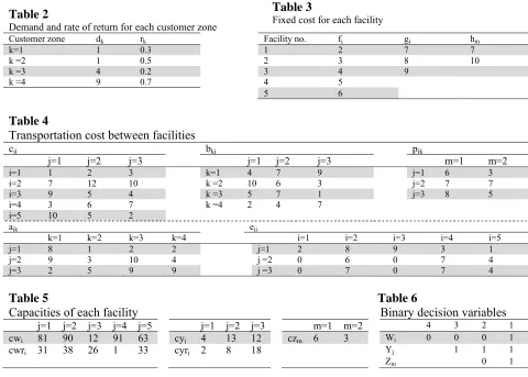
and were run on a core i5 Intel CPU with 4 GB of RAM. First, we assume a small-scaled integrated logistics network design with deterministic parameters to evaluate the priority-based genetic algorithm. Tables 2 to 5 give information about this problem and we assume that s=0.5.

Table 2

Demand and rate of return for each customer zone

Table 3

Fixed cost for each facility

Customer zone dk rk Facility no. fi gj hm

k=1 1 0.3 1 2 7 7

k =2 1 0.5 2 3 8 10

k =3 4 0.2 3 4 9

k =4 9 0.7 4 5

5 6

Table 4

Transportation cost between facilities

cij bkj pjk

j=1 j=2 j=3 j=1 j=2 j=3 m=1 m=2

i=1 1 2 3 k=1 4 7 9 j=1 6 3

i=2 7 12 10 k =2 10 6 3 j=2 7 7

i=3 9 5 4 k =3 5 7 1 j=3 8 5

i=4 3 6 7 k =4 2 4 7

i=5 10 5 2

ajk eji

k=1 k=2 k=3 k=4 i=1 i=2 i=3 i=4 i=5

j=1 8 1 2 2 j=1 2 8 9 3 1

j=2 9 3 10 4 j =2 0 6 0 7 4

j=3 2 5 9 9 j =3 0 7 0 7 4

Table 5 Table 6

Capacities of each facility Binary decision variables

j=1 j=2 j=3 j=4 j=5 j=1 j=2 j=3 m=1 m=2 4 3 2 1

cwi 81 90 12 91 63 cyj 4 13 12 czm 6 3 Wi 0 0 0 1

cwri 31 38 26 1 33 cyrj 2 8 18 Yj 1 1 1

Zm 0 1

First the model is solved by lingo 11, and a global optimum is reached in about 1 second. The related solution is shown in Table 6 and 8. Lingo uses a branch and bound approach and the objective value of the global optimum is 160.65.

Table 7

Transportation decision variables

Xij Qkj Tjk

j=1 j=2 j=3 j=1 j=2 j=3 m=1 m=2

i=1 4 10.75 0 k=1 0.5 0 0 j=1 0.3 0

i=2 0 0 0 k =2 0 0 0.69 j=2 0.345 0

i=3 0 0 0 k =3 0 0 1.12 j=3 0.27 0

i=4 0 0 0 k =4 1.5 2.3 0

i=5 0 0 1.75

Ujk Vji

k=1 k=2 k=3 k=4 i=1 i=2 i=3 i=4 i=5

j=1 0 0 4 0 j=1 1.7 0 0 0 0

j=2 0 1.25 0 9.5 j =2 1.95 0 0 0 0

j=3 1.25 0 0.5 0 j =3 1.54 0 0 0 0

(14)

Table 8

Comparison of 3 solving methods

Priority-based GA Classic GA Lingo No of constraints No. of variables M K J I Problem no. Time (sec.) Best Obj. Time (sec.) Best Obj. Time (sec.) Best Obj. 0.48 161.65 15 332 1 161.65 40 70 2 4 3 5 1 8.87 442.75 22 503 12 440.15 150 950 12 14 13 15 2 89.42 912 142 1930 114 1510 575 13415 55 45 50 60 3 233.53 2743.9 394 4735 * * 1150 53330 110 90 100 120 4

In problem no. 1 and 2 Lingo solver reached some optimal solution, which can be a basis to evaluate the two other methods. In problem no. 4 Lingo could not reach to a solution in reasonable amount of time. Therefore, it seems, priority-based genetic algorithm is a better efficiency choice for large-scaled cases. Now we solve a similar example but with hybrid parameters. Here, we assume that there are three scenarios (for example economic conditions) and estimate demand and rate of return under each scenario in terms of form of fuzzy variables based on expert's opinions. Table 9 gives information about demand (ξ_k) and rate of return (η_k). Probability of occurrence of each scenario (P1,P2,P3) which are predicted by historical data is shown in this table. Other information about this example is similar to previous problem.

Table 9

Fuzzy-random variables related to demand and rate of return of each customer zone

Customer zone

Scenario 1 P1=0.2

Scenario 2 P2=0.5

Scenario P3=0.5

k

ξ η_k ξ_k η_k ξ_k η_k

k=1 (0.5,1,1.5) (0.2,0.3,0.5) (1,2,3) (0.3,0.5,0.9) (2,4,6) (0.4,0.6,0.9)

k =2 (0.5,1,1.5) (0.05,0.4,0.5) (1,3,4) (0.1,0.4,0.7) (3,4,5) (0.2,0.5,0.7)

k =3 (3,4,5) (0.1,0.4,0.7) (3,6,8) (0.3,0.6,0.8) (5,8,10) (0.4,0.7,0.8)

k =4 (8,9,10) (0.2,0.3,0.5) (9,11,13) (0.3,0.5,0.9) (10,12,16) (0.4,0.6,0.9)

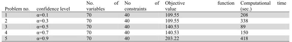
Now we solve this problem by the proposed fuzzy-random programming under several confidence level (α ) with this assumption that N=200. The results are shown in Table 10. As it seems, the objective function gets worse when we increase α.

Table 10

Results of hybrid programming for several confidence levels

Computational time (sec.) Objective function value No of constraints No. of variables confidence level Problem no. 208 109.55 40 70 α=0.1 1 338 109.55 40 70 α=0.3 2 89 140.53 40 70 α=0.5 3 150 140.53 40 70 α=0.7 4 418 203.22 40 70 α=0.9 5

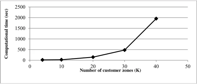
In this part, we solve the problem with a predefined confidence level and several number of customer zones to evaluate efficiency of the proposed hybrid programming under various scales. Table 11 illustrates the results and Fig. 6 depicts computational time versus each number of customer zones (K). Results from Table 11 represent that the proposed hybrid programming for integrated closed-loop logistics network design with fuzzy-random parameters is efficient for various scales.

Table 11

Results of hybrid programming for several number of customer zones (K)

Computational time (sec.) Objective function value No of constraints

(15)

As it seems in Fig. 6, by increasing the number of customer zones (K), computational times of solving the model increase, exponentially.

Fig. 6. Computational time versus each number of customer zones (K) 5. Conclusion

In this paper, we have considered a fuzzy-random mixed integer linear programming model for the design of an integrated forward/reverse logistics network with hybrid facilities. We have assumed that there are several scenarios (for example economic conditions) and estimated demand and rate of return under each scenario in the form of fuzzy variables by expert's opinion. Probability of occurrence of each scenario predicted by historical data and as a result, the demand and rate of return of customer zones have been regarded as fuzzy-random variables. In fact, this type of network design problem belongs to the class of NP-hard problems, so that we have utilized the priority-based genetic algorithm known to be an efficient and robust method for this kind of problem. A hybrid programming approach by fuzzy-random simulation has been applied to solve the uncertain model. Some examples are introduced in several scales and results showed that the proposed method solves them efficiently. Develop the hybrid model for multi-product or multi-period, using multi-objective programming to consider customer satisfaction for this problem can be subjects for future researches.

References

Altiparmak, F., Gen, M., Lin, L., & Karaoglan, I. (2009). A steady-state genetic algorithm for multi-product supply chain network design. Computers & Industrial Engineering, 56, 521–537.

Altiparmak, F., Gen, M., Lin, L., & Paksoy, T. (2006). A genetic algorithm for multi-objective optimization of supply chain networks. Computers & Industrial Engineering, 51, 197–216.

Barros, A. I., Dekker, R., & Scholten, V. (1998). A two-level network for recycling sand: a case study. European Journal of Operational Research, 110, 199–214.

Charnes, A., & Cooper W. (1961). Management Models and Industrial Applications of Linear Programming.

Wiley, New York.

Du, F., & Evans, G. W. (2008). A bi-objective reverse logistics network analysis for post-sale service.

Computers and Operations Research, 35, 2617 – 2634.

Gen, M., Altiparmak, F., & Lin, L. (2006). A genetic algorithm for two-stage transportation problem using priority-based encoding. OR Spectrum, 28, 337–354.

Gen, M., & Cheng, R. (2000). Genetic algorithms and engineering optimization. John Wiley and Sons, New

York.

Gen, M., & Syarif, A. (2005). Hybrid genetic algorithm for multi-time period production/distribution planning.

Computers & Industrial Engineering, 48, 799–809.

Huang, X. (2006). Optimal project selection with random fuzzy parameters, International Journal of Production Economics, 112-122.

Jaramillo, J. H., Bhadury J, & Batta, R. (2002). On the use of genetic algorithms to solve location problems.

Computers and Operations Research, 29, 761-779.

0 500 1000 1500 2000 2500

0 10 20 30 40 50

Com

put

at

ional t

im

e (

sec

)

(16)

Jayaraman, V., Guide, V. D., & Srivastava, R. (1999). A closed loop logistics model for remanufacturing.

Journal of the Operational Research Society, 50, 497–508.

Jayaraman, V., Patterson, R. A., & Rolland, E. (2003). The design of reverse distribution networks: Models and solution procedures. European Journal of Operational Research, 150, 128–149.

Kara, S., Rugrungruang, F., & Kaebernick, H. (2007). Simulation modeling of reverse logistics networks.

International Journal of Production Economics,106, 61–69.

Kim, K., Song, I., Kim, J., & Jeong, B. (2006). Supply planning model for remanufacturing system in reverse logistics environment. Computers & Industrial Engineering, 51, 279–287.

Kirkke, H. R., Harten, A. V., & Schuur, P. C. (1999). Business case Oce: reverse logistic network redesign for copiers. OR Spectrum, 21,381–409.

Ko, H. J., & Evans, G. W. (2007). A genetic algorithm-based heuristic for the dynamic integrated forward/reverse logistics network for 3PLs. Computers and Operations Research, 34, 346–366.

Kwakernaak, H. (1978). random variables: Definitions and theorems. 15, 1-29.

Lee, D.H., & Dong, M. (2008). A heuristic approach to logistics network design for end-of-lease computer products recovery. Transportation Research Part E, 44, 455-474.

Lee, J. E., Gen, M., & Rhee, K. G. (2009). Network model and optimization of reverse logistics by hybrid genetic algorithm. Computers & Industrial Engineering, 56, 951–964.

Liu, B. (2001). Fuzzy random chance-constrained programming, IEEE Transactions on Fuzzy Systems, 9(5),

713-720.

Liu, B. (2002a). Random fuzzy dependent-chance programming and its hybrid intelligent algorithm, Information Sciences, 141 (3–4), 259–271.

Liu, B. (2002b). Theory and Practice of Uncertain Programming, Physica-Verlag, Heidelberg.

Liu, B. (2006). Theory and Practice of Uncertain Programming. Beijing, China: Uncertainty Theory

Laboratory- Department of Mathematical Sciences-Tsinghua University.

Liu, B. (2009). Theory and Practice of Uncertain Programming (3rd ed.). Beijing, China: Uncertainty Theory

Laboratory- Department of Mathematical Sciences-Tsinghua University.

Liu, B., Iwamura, K. (1998). Chance constrained programming with fuzzy parameters, Fuzzy Sets and Systems,

94, 227–237.

Liu, Y., & Liu, B. (2003). A class of fuzzy random optimization: Expected value models. Information Sciences, 155, 89-102.

Liu, Y., & Liu, B. (2003). Expected value operator of random fuzzy variable and random fuzzy expected value models, International Journal of Uncertainty, Fuzziness and Knowledge-Based Systems 11 (2), 195–215.

Lu, Z., & Bostel, N. (2007). A facility location model for logistics systems including reverse flows: The case of remanufacturing activities. Computers and Operations Research, 34: 299–323.

Michalewicz, Z., Vignaux, G. A., & Hobbs, M. (1991). A non-standard genetic algorithm for the nonlinear transportation problem. ORSA Journal on Computing, 3, 307–316.

Min, H., Ko, H. J., & Ko, C. S. (2006). A genetic algorithm approach to developing the multi-echelon reverse logistics network for product returns. Omega, 34, 56 – 69.

Min, H., Ko, H. J., & Park, B. I. (2005). A Lagrangian relaxation heuristic for solving the echelon, multi-commodity, closed-loop supply chain network design problem. International Journal of Logistics Systems and Management, 1, 382–404.

Pishvaee, M. S., Jolai, F., & Razmi, J. (2009). A stochastic optimization model for integrated forward/reverse logistics A stochastic optimization model for integrated forward/reverse logistics. Journal of Manufacturing Systems, 107-114.

Pishvaee, M. S., Zanjirani Farahani, R., & Dullaert, W. (2010). A memetic algorithm for bi-objective integrated forward/reverse logistics network design. Computers & Operations Research, 37, 1100-1112.

Shen, Z.M. (2007). Integrated supply chain design models: a survey and future research directions. Journal of Industrial and Management Optimization, 3(1),1-27.

Syarif, A., Yun, Y. S., & Gen, M. (2002). Study on multi-stage logistic chain network: a spanning tree-based genetic algorithm approach. Computers & Industrial Engineering, 43, 299-314.

Wen, M., & Iwamura, K. (2008). Facility location–allocation problem in random fuzzy environment: Using (α,β)-cost minimization model under the Hurewicz criterion. Computers & Mathematics with Applications, 55(4), 704-713.

Xu, J., Liu, Q., & Wang, R. (2008). A class of multi-objective supply chain networks optimal model under random fuzzy environment and its application to the industry of Chinese liquor. Information Sciences, 178,