Novel Pitch Detection Algorithm With Application to Speech Coding

ScholarWorks@UNO

ScholarWorks@UNO

University of New Orleans Theses and

Dissertations Dissertations and Theses

12-19-2003

Novel Pitch Detection Algorithm With Application to Speech

Novel Pitch Detection Algorithm With Application to Speech

Coding

Coding

Vijay Kura

University of New Orleans

Follow this and additional works at: https://scholarworks.uno.edu/td

Recommended Citation Recommended Citation

Kura, Vijay, "Novel Pitch Detection Algorithm With Application to Speech Coding" (2003). University of New Orleans Theses and Dissertations. 52.

https://scholarworks.uno.edu/td/52

This Thesis is protected by copyright and/or related rights. It has been brought to you by ScholarWorks@UNO with permission from the rights-holder(s). You are free to use this Thesis in any way that is permitted by the copyright and related rights legislation that applies to your use. For other uses you need to obtain permission from the rights-holder(s) directly, unless additional rights are indicated by a Creative Commons license in the record and/or on the work itself.

APPLICATION TO SPEECH CODING

A Thesis

Submitted to the Graduate Faculty of the University of New Orleans in partial fulfillment of the requirements for the degree of masters

Master of Science in

The Department of Electrical Engineering

by

Vijay B. Kura

B.Tech., Jawaharlal Institute of Technological University, 2000

TABLE OF CONTENTS

LIST OF ILLUSTRATIONS……… v

List of Figures……… vi

List of Tables……… vii

Glossary of Abbreviations……… viii

ABSTRACT……… ix

1. INTRODUCTION……… 1

1.1Motivation to speech coding……… 1

1.2Importance of Pitch to speech coding……… 2

1.3Thesis Contribution……… 4

1.4Thesis Outline……… 4

2. SPEECH PRODUCTION AND PERCEPTION……… 6

2.1 Human Speech Production……… 6

2.1.1 Mechanism of Speech Production……… 7

2.1.2 Sub-glottal system……… 8

2.1.3 Vocal tract……… 8

2.2. Factors Influencing the Fundamental frequency……… 9

2.3. Speech analysis……… 12

2.3.1 Fundamental frequency estimation……… 12

2.3,2 Spectral analysis……… 14

2.3.3 Wavelet analysis……… 15

2.3.4 Cepstrum analysis……… 16

3. SPEECH CODERS AND CLASSIFICATION……… 18

3.1 Algorithm Objectives and Requirements……… 19

3.2 Speech coding Strategies and Standards……… 22

3.3 Waveform Coders……… 22

3.3.1 Pulse Code Modulation……… 24

3.4 Voice Vocoders……… 27

3.5 Hybrid Coders……… 28

3.5.1 Time-domain Hybrid Coders……….. 28

3.5.1.1 The Basis LPC Analysis by Synthesis Model……… 29

3.5.2.1 Code Excited Linear Predictive coding……… 34

3.5.2.2 Multipulse-Excited LPC……… 35

4. LINEAR PREDICTION OF SPEECH……… 37

4.1 Linear Prediction in speech coding……… 37

4.1.1 Role of Windows……… 42

4.1.2 LP coefficient computation……… 43

4.1.3 Gain computation……… 45

4.2. LPC vocoder……… 46

5. PITCH ESTIMATION AND PITCH ESTIMATION ALGORITHMS……… 48

5.1 Back Ground……… 48

5.1.1. Applications of pitch estimation……… 48

5.1.2 Importance of pitch estimation in Speech coding……… 49

5.1.3 Difficulties in estimation of pitch estimation……… 50

5.2 Non-Event Pitch detectors……… 51

5.2.1 Time domain waveform similarity method……… 51

5.2.1(a). Auto-correlation PDA……… 52

5.2.1(b) Average Magnitude Difference Function PDA………… 53

5.2.2 Frequency domain spectral similarity methods……… 54

5.2.2(a) Harmonic Peak detection………. 55

5.2.2(b) Spectrum Similarity……… 56

5.2.2(c) Cepstrum peak detection……… 58

5.3. Event pitch detectors……… 59

5.3.1 Wavelet based PDA……… 59

6. A NOVEL WAVELET-BASED TECHNIQUE FOR PITCH DETECTION AND SEGMENTATION OF NON-STATIONARY SPEECH… 63 6.1. Proposed technique……… 64

6.1.1 The feature extraction and ACR stages……… 65

6.1.2 Pitch detection under noisy conditions……… 68

6.2.4 Advantages of MAWT in speech segmentation and modeling…… 68

6.2. Results……… 70

7. Conclusions……… 73

Reference……… 74

VITA……… 77

Acknowledgements

First of all I want to express my gratitude to my advisor Dr. Dimitri Charalampidis for his invaluable guidance during the entire period of this work. I’m very obliged for his suggestions,

ideas and concepts without which this work wouldn’t have been what it is now.

I also would like to thank my committee members Dr. Vesselin Jilkov, Dr. Jing Ma and Dr. Terry Remier for their suggestions and insightful comments

Finally I would like to thank my parents and my family for their continuous and

unconditional love and support

.

List of Illustrations

List of figures:

Figure 2.1 Schematic view of human speech production mechanism.

Figure 2.2 Block diagram of human speech production

Figure 2.3 Average spectral trends of the sound source, sound modifiers and lip radiation during

voiced (V+) and voiceless (V-) speech.

Figure 2.4 (a) Laryngeal shape of female and male speaker (b) Relative sizes of the laryngeal Figure 2.5 Model spectrogram of “what do you think about that” spoken by the healthy adult

female.

Figure 3.1 Classification of speech coding schemes Figure 3.2 Quality comparison of speech coding schemes

Figure 3.3 µ-law companding function µ=0 ,4,16…256.

Figure 3.4. Block diagram of a logarithmic encoder-decoder

Figure 3.5 General structure of an LPC-AS coder (a) and decoder (b). LPC filter A(z) and

perceptual weighting filter W(z) are chosen open-loop, then the excitation vector u(n) is chosen in closed-loop fashion in order to minimize the error metric |E|2.

Figure 3.6 Generalised block diagram of AbS-LPC coder with different excitation types

Figure 3.7 Multipulse-Excitation Encoder Figure 4.1 Modeling speech production Figure 4.2 LP Analysis and synthesis model

Figure 4.3 LPC Vocoder

Figure 5.1 (a) Original Speech signal, (b) auto-correlation function and (c) AMDF

Figure 5.2Original spectra and Synthetic spectra used in the Harmonic Peak Detection PDA method

Figure 5.3 Original spectra and Synthetic spectra used in the spectrum similarity PDA method

Figure 5.4 (a) Input Speech waveform (b) Log spectrum of the speech waveform and (c) Ceptsrum of the speech waveform

Figure 5.5 DyWT of the part of the signal /do you/ spoken by the female speaker using SPLINE

wavelet (a) computed with scale a=22 (b) computed with scale a=23 (c) computed with scale a=24 (d) computed with scale a=25 (e) Original signal with stars and square indicates the locations of local maximum which greater than 0.8 time global maximum Figure 6.1 Proposed pitch detection scheme.

Figure 6.2 Example of pitch estimation. (a) Non-stationary fundamental frequency component using MAWT’s wavelet stage, and (b) corresponding successful pitch estimation results. (c),(d) Two consecutive scales of the wavelet transform, and (e)

corresponding successful pitch estimation results.

Figure 6.3 Example of pitch estimation for gain-varying signal. (a) Non-stationary fundamental frequency component using MAWT’s wavelet stage, and (b) corresponding

successful pitch estimation results. (c),(d) Two consecutive scales of the wavelet transform, and (e) Corresponding unsuccessful pitch estimation results.

List of Tables:

Table 1.1 Typical first three formant frequency ranges f0 mean and ranges of conversational

speech of man, women and children (formant values from [4]). Table 2.1 representation of speech coding standards

Table 6.1 Comparison in terms of estimation error percentage for various noise levels

Glossary of Abbreviations

PCS Personal Communication Systems VOIP Voice Over Internet Protocol

DSVD Digital Simultaneous Voice and Data

NB Narrowband

WB Wideband

PSTN Public Switched Telephone Networks ASIC Application Specific Integrated Circuits

FEC Forward Error Correction MOS Mean Square Score PCM Pulse Code Modulation

ADPCM Adaptive Pulse Code Modulation DAM Diagnostic Acceptability Measure

DRT Diagnostic Rhyme Test AbS Analysis by Synthesis STP Short-time Predictor

LTP Long-time Predictor

CELP Code Excited Linear Predictive coding

RPELPC Regular Pulse Excitation LPC LPC Linear Predictive Coder

RELP Residual Excitation Coding

RPE Regular Pulse Excitation coding SELP Self Excitation Coding

MELP Mixed Excitation Linear Predictive Coding

MBE Multi-Band Excitation Coder SNR Signal-to-Noise ration MSE Mean Square Error

ARMA Auto Regressive Moving Average

ACR Auto-Correlation

AMDF Average Magnitude Difference Function PDA Pitch Detection Algorithms

GCI Glottal Closure Instant

MLE Maximum Likelihood Estimation

MAWT Multi-feature, Autocorrelation (ACR) and Wavelet Technique

STE Short-time Energy

ZCR Zero-Crossing Rate

ABSTRACT

This thesis introduces a novel method for accurate pitch detection and speech segmentation, named Multi-feature, Autocorrelation (ACR) and Wavelet Technique (MAWT). MAWT uses

feature extraction, and ACR applied on Linear Predictive Coding (LPC) residuals, with a wavelet-based refinement step. MAWT opens the way for a unique approach to modeling:

although speech is divided into segments, the success of voicing decisions is not crucial. Experiments demonstrate the superiority of MAWT in pitch period detection accuracy over existing methods, and illustrate its advantages for speech segmentation. These advantages are

more pronounced for gain-varying and transitional speech, and under noisy conditions.

Chapter 1: Introduction

1.1 Motivation for Speech Coding

Speech communication is arguably the single most important interface between humans, and it is now becoming an increasingly important interface between human and machine. As

such, speech represents a central component of digital communication and constitutes a major driver of telecommunications technology. With the increasing demand for telecommunication

services (e.g., long distance, digital cellular, mobile satellite, aeronautical services), speech coding has become a fundamental element of digital communications. Emerging applications in rapidly developing digital telecommunication networks require low bit, reliable, high quality

speech coders. The need to save bandwidth in both wireless and line networks, and the need to conserve memory in voice storage systems are two of the many reasons for the very high activity

in speech coding research and development. New commercial applications of low-rate speech coders include wireless Personal Communication Systems (PCS) and voice-related computer applications (e.g., message storage, speech and audio over internet, interactive multimedia

terminals). In recent years, speech coding has been facilitated by rapid advancement in digital signal processing and in the capabilities of digital signal processors. A strong incentive for

for larger capacity of the telecommunication networks. Nevertheless, the rapid advancement in

the efficiency of digital signal processors and digital signal processing techniques has stimulated the development of speech coding algorithms. These trends are likely to continue, and speech compression most certainly will remain an area of central importance as a key element in

reducing the cost of operation of voice communication systems.

1.2 Importance of Pitch Estimation in Speech Coding

The motivation for speech coding is to reduce the cost of operation of voice

communication that involves development of various efficient coding algorithms and relating areas. One of the important areas of speech coding is pitch estimation. There is a significant

number of speech coding algorithms, which are broadly classified into four categories, namely, phonetics, waveform, hybrid and voice vocoders. A detail explanation of these coders is presented in the [Chapter 3]. Phonetics vocoders are more related to the acoustic characteristics

of speech signals, whose investigation is beyond the scope of this thesis. Second form coders are waveform coders, which are based on a simple sampling and amplitude quantization process.

These coders include 16-bit PCM [19], companded 8-bit PCM [19], and ADPCM [18]. Since the only concept behind these coder types is amplitude quantization, the compression rate of speech signals is limited to very large numbers. Even the most recently standardized waveform coders

require a minimum of 16 kbits/sec. However, the main objective of the current speech coders is to reduce the minimum compression rate to 1 - 4 kbits/sec or even lower. With the increasing

applications, simple amplitude quantization is not an efficient process for transmission of speech

signals.

In contrast to waveform coders, vocoders consider the details in the nature of human speech. In their principles, there is no attempt to match the exact shape of the signal waveform.

Vocoders generally consist of an analyzer and synthesizer. The analyzer attempts to estimate and then transmit the model parameters that represent the original signal. Speech is synthesized using

these parameters to produce an often crude and synthetic constructed speech signal. These types of algorithms are called perceptual quality coders. A very familiar and traditional speech vocoder is LPC-10e. In this type of coders, speech signals are synthesized with an excitation that consists

of a periodic pulse train or white noise. The complete quality of the synthesized speech signal depends on the excitation signal. The excitation is simply a train of narrow pulses. Two

consecutive pulses are placed apart by a time difference equal to the pitch period. Therefore, the quality of the synthesized speech signal highly depends on the accurate estimation of the pitch period.

Even the most recently developed algorithms, such as MPLPC [35], RPELPC [36], CELP

[26], require the correct estimation of the LP coefficients, LTP coefficients and excitation. The basis for estimating these parameters is the fundamental pitch period. Incorrect estimation of the fundamental period harms the estimation of the LTP coefficients, and consequently, the residual.

This in turn causes an incorrect selection of excitation, therefore the final speech quality.

toll-quality, communication toll-quality, professional quality or synthetic toll-quality, it all depends on the

correct estimation of fundamental pitch.

1.4 Thesis Contribution

The following section describes the contribution of the thesis

The new proposed pitch estimation algorithm based on Gabor filters, and an efficient implementation of the auto-correlation method is presented in the chapter 6. This technique is

named as Multi-feature, Autocorrelation (ACR) and Wavelet Technique (MAWT). The algorithm has moderate advantages over all the traditional and most recently PDA’s for speech

signals with or without noise. The accuracy of pitch estimation for fast pitch changing signals, for low energy speech signals, and for transition is improved. The algorithm is threshold insensitive and independent of frame length. Other contributions of the thesis are the study and

comparison of various speech coding algorithms, and the complete implementation of LPC vocoder and MBE vocoder. In addition to the above, the reason why pitch estimation of speech

signal plays vital role in the final quality of synthesized signal is highlighted.

1.5 Thesis Outline

Chapter 2 presents a thorough description of the basic speech production mechanism and provides the background information for understanding the major contribution of this thesis. It

provides a description of the main speech coder categories and their principles and concepts. It

also includes the complete description of the components involved in a generalized model. This description gives the basis of the importance of the pitch estimation in speech coding. Chapter 4 discusses the difficulties in pitch estimation, and includes the complete methodology of some

traditional and some recently developed pitch detection algorithms. Finally, chapter 5 presents a novel pitch detection algorithm, named MAWT. A comparison between the methods presented

Chapter 2: Human Speech Production and Perception

This chapter provides an introductory description of the principles related to speech production and perception of speech. First, human speech production is described from the basic

acoustic point of view, and second, through the introduction of the factors influencing the fundamental pitch period. Finally, a spectral analysis of speech production is presented, and different fundamental pitch estimation methods are briefly discussed.

2.1 Human Speech Production

Speech signals are composed of a sequence of sounds. These sounds and the transition between them serve as a symbolic representation of information. The arrangement of sounds (symbols) is governed by the rules of the language. The study of the rules and classification of

speech is called phonetics. The purpose of processing speech signals is to enhance and extract information, which is helpful in providing as much knowledge as possible about the signal’s

2.1.1 The mechanism of speech production

Human speech production requires three elements – a power source, a sound source and sound modifiers. This is the basis of the source-filter theory of speech production. The power source in normal speech results from a compression action of the lung muscles. The sound

source, during the voiced and unvoiced speech, results from the vibrations of the vocal folds and turbulent flow past narrow constriction respectively. The sound modifiers are the articulators,

which change the shape and therefore the frequency characteristics of the acoustic cavities through which the sound passes.

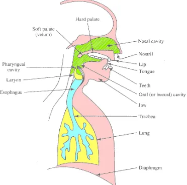
The main anatomy of the human speech production mechanism is depicted in figure 2.1

and an ideal block diagram of the functional mechanism is illustrated in the figure 2.2. The three main controls of the speech production are –lungs (power source), the position of the vocal folds

(sound source) and the shape of the vocal tract (sound modifiers).

Figure 2.1 Schematic view of human speech production mechanism.

2.1.2 Sub-glottal system

This system is composed of the lungs, and the vocal folds. This sub-glottal system serves as a power source and sound source for the production of speech. Speech is simply an acoustic wave radiated from the sub-glottal system, when the air is expelled from the lungs and the

resulting flow of air is perturbed by a constriction somewhere in the vocal tract. Speech sounds can be classified into three distinct classes according to their mode of excitation:

• Voiced sounds are produced by forcing air through the glottis with tension of the vocal cords adjusted so that they vibrate in a relaxation oscillation, there by producing quasi-periodic pulses of air which excite the vocal tract.

• Unvoiced or fricative sounds are generated by forming a constriction at some point in the vocal tract (usually toward mouth end) and forcing air through the constriction at high

enough velocity to produce turbulence.

• Plosive sounds result from making a complete closure (again usually toward the front of the vocal tract), building up pressure behind the closure and abruptly releasing it.

2.1.3 Vocal tract

The vocal tract is also termed as sound modifiers, and it is depicted in figure 2.2. It is

formed by the oral together with the nasal cavities. The shape of the vocal tract (but not the nasal cavity) can be altered during speech production that changes its acoustics properties. The velum can be raised or lowered to shut off or couple the nasal cavity, and then the shape of the vocal

frequency response curve known as formants. Depending upon the shape of the vocal tract tube,

the first three formant frequencies for men, women and children are given in table 2.1.

Parameter Men Women Children F1 range 270 Hz – 730 Hz 300 Hz – 800 Hz 370 Hz – 1030 Hz

F2 range 850 Hz – 2300 Hz 900 Hz – 2800 Hz 1050 Hz – 3200 Hz F3 range 1700 Hz – 3000 Hz 1950 Hz – 3300 Hz 2150 Hz – 3700 Hz

f0 mean 120 Hz 225 Hz 265 Hz

Table 2.1 Typical first three formant frequency ranges f0 man and ranges of conversational

speech of mean, women and children (formant values from [4]).

The average frequency domain effects in speech production are summarized in figure 2.3. Human speech has an approximate 6 dB per octave roll-off with increasing frequency.

The sound source and the sound modifiers make the following contributions to this spectrum. For voiced speech, all harmonics are present with an average spectral roll-off of 12 dB per octave, while for voiceless speech the spectrum is flat. Radiation of the acoustic pressure

waveform via the lips gives a +6dB per octave tilt with increasing frequency. This results in an average overall spectral variation with increasing frequency during voiceless speech. Since the amplitude of voiced speech is usually significantly greater than that of voiceless speech, the

average spectral shape of speech tends to be close to –6 dB per octave.

0 dB/octave +6 dB/octave V+ -6 dB/octave V-: + 6 dB/ocatve Sound

modifiers lip radiation _output

V+ -12 dB/octave V-: 0 dB/ocatve

Sound source

2.2. Factors Influencing the Fundamental frequency

This section explains some of the physiological factors, as well as other factors that influence pitch.

(a) Body size

The most obvious influence on pitch that comes to mind is the size of the sound-producing apparatus; we can observe from the instruments of the orchestra that smaller objects

tend to make higher-pitched sounds, and larger ones produce lower-pitched sounds. Therefore, it is logical to assume that small people would make high sounds, and large people would make low sounds. And this assumption is borne out by the facts, at least to an extent. Baby cries have a

fundamental frequency (referred to as f0) of around 500 Hz. Child speech ranges from 250-400

Hz, adult females tend to speak at around 200 Hz on average and adult males around 125 Hz.

Thus, the body size is one of the factors related to f0. On the other hand, we know that big opera

singers don't always make low sounds; there are very large sopranos, and some rather short, slender basses. So, body weight and height is not a sole determining factor.

(b) Laryngeal size

Perhaps, a factor more relevant to the voice source is the size of the larynx. Men, on

average, have a larynx about 40% taller and longer (measured along the axis of the vocal folds) than women, as seen in figure 2.4. Nevertheless, this does not completely explain the difference between male and female fundamental frequency f0; there is a size difference inside the larynx,

Figure 2.4 (a) Laryngeal shape of female and male speaker (b) Relative sizes of the laryngeal

(c) Vocal fold length

If it is assumed that the vocal folds are 'ideal strings' with uniform properties, their

fundamental frequency f0 is governed by Equation 2.1.

ρ σ

L F

2 1

0 = 2.1

where

L: Length of vocal folds σ: Longitudinal stress ρ: Tissue density

The key variable here is the length of the vocal folds part that is actually in vibration,

found that men have a 60% longer effective fold length than women, on average, which accounts

for the general f0 difference observed between the sexes.

Briefly, some other factors that influence the fundamental pitch period are (1) the difference between languages (2) the specifics of different applications, (3) the emotional state of

the person and (4) the environmental conditions under which speech is produced.

2.3. Speech analysis

One of the important characteristics of a speech waveform is the time-varying nature of the content of the speech pressure. Determination of the time-varying parameters of speech is a key area of analysis required in speech research. Another key area is classification of speech

waveform segments into voiced or voiceless (mixed excitation is usually considered voiced). As mentioned previously, in the case where speech is voiced, the most important parameter is the

fundamental frequency value f0.

This section introduces these two areas of analysis and discusses the principles and limitation involved. First, the fundamental frequency f0 analysis is considered, followed by the

spectral analysis method of dynamic speech signals.

2.3.1 Fundamental frequency estimation

The pitch of a sound depends on how our hearing system functions and is based on a subjective judgment by a human listener on a scale from low to high. Therefore, such a psychoacoustic measurement cannot currently be made algorithmically without the involvement

of a human listener. The f0 measurement of the vocal fold vibration is an objective measure,

be preferred to the term pitch extraction commonly used in the literature. One reason why

estimation rather than extraction is adopted, is that although changes in pitch are perceived when f0 is varied, small changes in pitch can also be perceived when the intensity (loudness) or the

sound’s spectral content (timbre) is varied when f0 is kept constant.

The choice of an f0 measurement technique should be made with direct reference to the

particular demands of the intended application in terms of the expected speaker population to be

analyzed (adult or child, male or female, pathological or non-pathological), the likely competition from acoustic back ground or foreground noise (others working in the same room, external noises, domestic noises, machine noises, classroom, clinic, children), the material to be

analyzed (read speech, conversation speech, shouting, sustained vowel, singing), the effect of the speaker to analysis system signal transmission path (room acoustics, microphone placement,

telephone, pre-amplification) and the measurement errors can be tolerated (f0 doubling, f0

halving, f0 smoothing, f0 jitter).

The operation of f0 estimation algorithms can be considered in terms of

• The input pressure waveform (time domain)

• The spectrum of the input signal (frequency domain)

• A combination of time and frequency domains (hybrid domain) • Direct measurement of larynx activity

Most of the errors associated with f0 estimation are due to

• The difficulties in locating accurately the onsets and offsets of voiced segments

A highly comprehensive review is given in Hess [5], some of the methods of estimation, errors involved and importance to speech coding will be discussed in chapter (5)

2.3.2 Spectral analysis

Since the 1940’s, the time-varying spectral characteristics of the speech signal can be graphically displayed through the use of the sound spectrograph [32,33]. This device produces a

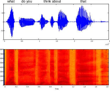
two-dimensional pattern called a spectrogram in which the vertical dimension corresponds to frequency and horizontal dimension to time. The 16 bit gray scale level is used to represent the given spectrogram. Even though the color representation is more visually appealing, it

sometimes leads to misleading interpretation of the spectrogram. The darkness of the pattern is proportional to signal energy. Thus, the resonance frequencies of the vocal tract show up as dark

bands in the spectrogram. Voiced regions are characterized by a striated appearance due to the periodicity of the time waveform, while the unvoiced intervals more solidly filled in. An example, spectrogram of the utterance of “What do you think about that” of a female speaker (in

the Figure 2.5a) is shown in the Figure 2.5b. The spectrogram is labeled corresponds to the labeling of Figure 2.5b, so that the time domain and frequency domain can be correlated.

The time scale and frequency resolution of the spectrograph plays a vital role in representation of speech spectral energy. The most rapid changes in time scale occur during the release stages of plosives, which order is of 5-10ms. For individual representation of the

harmonics of male speech, a frequency resolution less than the minimum expected f0 for males –

between frequency and time resolution and this can be controlled by altering the bandwidth of

the spectrograph’s analysis filter. Usually, this is indicated as wide or narrow based on the relation between the filter’s bandwidth and the f0 of the speech being analyzed.

0 0.5 1 1.5 2 2.5 3

x 104 -1

-0.5 0 0.5 1

Time

0 0.2 0.4 0.6 0.8 1 1.2 1.4 1.6 1.8

0 1000 2000 3000 4000 5000 6000 7000 8000

what do you think about that

Fig 2.5 Model spectrogram of “what do you think about that” spoken by the healthy adult female.

2.3.3 Wavelet analysis

bandwidth filters. The resulting computation structure is very similar to the tree-structured

quadrature filter bank used in speech coding.

In fact, the quadrature-mirror filterbank is form of wavelet transform with the output samples of the filters representing the transform coefficients. Due to the variable bandwidth,

which is proportional to frequency, the basis functions are simply rescaled and shifted versions of each other in time.

One of the important characteristics of wavelet transforms, in addition to their variable bandwidth characteristics, is that they are simultaneously localized in time and frequency which allows them to possess, at the same time, the desirable characteristics of good time and

frequency resolution.

2.3.4 Cepstral analysis

One of the problems of simple spectral analysis is that the resulting output has elements of both the vocal tract (formants) and its excitation (harmonics). This mixture is often confusing and inappropriate for further analysis, such as speech recognition. Ideally, some method of

separating out the effects of the vocal tract and the excitation would be appropriate.

Unfortunately, these two speech aspects are convolved together and they cannot be separated by

simple filtering. One speech analysis approach that can help in separating the two elements is the Cepstrum[12]. This finds applications both pitch detection and vocal tract.

The method relies on applying nonlinear operations to map the operation of convolution

This is achieved via two mappings

• Convolution in the time domain is equal to multiplication in the frequency domain • The sum of the logarithms of two numbers is equal to the logarithm of their product.

Thus, Fourier transforming a signal representing two convolved signals, and then taking

the logarithm, results in a transform, which represents the sum of two convolved signals. This additively resulted can then be transformed back to the time domain and processed to separate

Chapter 3: Speech coders and Classification

The purpose of this chapter is to introduce various speech coder standards, their requirements, and their evolution. A broad categorization and the brief explanation of different

categories are presented. Finally, some of speech coders are discussed in detail.

Speech coding is the process of obtaining a compact representation of voice signals for

efficient transmission over band-limited wired and wireless media and/or storage. Today, speech coders have become essential components in telecommunications and in the multimedia infrastructure. Commercial systems that rely on efficient speech coding include cellular

communication, voice over internet protocol (VOIP), videoconferencing, electronics toys, archiving, and digital simultaneous voice and data (DSVD), as well as numerous PC-based games and multimedia applications.

Speech coding is the art of creating a minimally redundant representation of the speech signal that can be efficiently transmitted or stores in digital media, and decoding signal with the

best possible perceptual quality. Like any other continuous-time signal, speech may be represented digitally through the processes of sampling and quantization; speech typically quantized using either 16-bit uniform or 8-bit companded quantization. Like many other signals,

however, a sampled speech signal contains a great deal of information between either redundant (nonzero mutual information between successive samples) or perceptually irrelevant

meaning that the synthesized speech is perceptually similar to the original but may be physically

dissimilar.

A speech coder converts a digitized speech signal into a coded representation, which is usually transmitted in frames. A speech decoder receives coded frames and synthesizes

reconstructed speech. Speech coders may differ primarily in bit rate (measured in bits per sample or bits per second), complexity (measured in operations in seconds), delay (measured in

miiliseconds between recording and playback) and perceptual quality of the synthesized speech. Narrowband (NB) coding refers to speech signals whose bandwidth is less than 4 kHz (8kHz sampling rate), while wideband (WB) coding refers to coding of 7-kHz bandwidth signals (14-16

kHz sampling rate). NB coding is more common than WB coding mainly because of the narrowband nature of the wireless telephone channel (300-3600 Hz). More recently, however,

there has been an increased effort in wideband speech coding because of several applications such as videoconferencing.

Section 1 discusses the speech coder requirements and objectives, followed by the section

2, which discusses the broad classification of the speech coders. The rest of the sections 3, 4, and 5, give the detail explanation of above speech coders.

3.1. Algorithm Objectives and requirements

The design and capacity of a particular algorithm often depends upon the target

application. Sometimes capacity of the algorithms is bounded by stringent network planning rules, in order to maintain high quality of service and not to degrade the existing service. There

(i) Speech quality: The speech coding consideration is speech quality against the bit rate.

The lower the bit rate i.e., the higher the signal compression, the more the quality suffers. How to determine the speech quality is still a matter question. However, other factors that affect the requirements for obtaining the appropriate speech quality are the type of application, the

environment and the type of the network technology.

(ii) Coding delay: Coding delay includes algorithmic (the buffering of speech for

analysis), computational (time taken to process the stored speech samples) and transmission factors. Delay becomes a problem for two reasons. Firstly, speech coders are often interfaced to the PSTN via four to two wire converters or "hybrids". A side effect of using these devices is

that a proportion of the output signal from the codec is fed back into the input of the codec. Due to coding delays, this introduces echo. This is extremely disconcerting to the user, who hears one

or more echoes of his own voice returned at multiples of 80-120 ms. The second problem with delay is when the coding delay is coupled with long transmission delays such as those encountered with transmission via satellites in geosynchronous orbit (200 ms round trip). In this

case, a total delay of over 300 ms may be encountered, making actual conversation difficult. Thus minimization of coding delay is an important research aim.

(iii) Computational complexity and cost: Lowering the bit rate while maintaining quality is often achieved at the expense of increased complexity. A complex algorithm requires powerful DSP hardware that is expensive and requires increased power consumption. Until the late 1980's,

many speech coding algorithms were not implementable in real time due to the lack of sufficiently powerful real time DSP hardware. The advent of the digital signal processors (DSP)

hardware is an important factor. Thus, the search for computationally efficient algorithms is an

important research activity to reduce DSP hardware requirements, power consumption, and cost of speech coding hardware.

(iv) Robust to Channel errors: For many applications, the quality of speech signals

against the channel error, being accomplished by employing the Forward Error Correction (FEC). However, it is important to maintain the acceptable quality for mobile and satellite

systems, which suffer from random and burst types of noise. The disadvantage with use of FEC is that extra bandwidth is required and that it is unacceptable for mobile and satellite systems. Thus the robustness to channel error is an important consideration.

(v) Robust to Background noise: Most of the low-bit rate speech coders exploit the

redundancy in the speech signals. However redundancy is not necessarily the same for other

signals such as background noise or single sinusoids. In such cases, the speech coder may distort or corrupt the synthesized speech signals. Another effect is that the signal processing techniques used to extract model parameters may fail when speech corrupted by high levels of background

noise is coded. For example, many of the very low rate, synthetic quality vocoders used by the military fail in moving vehicles or helicopters due to the presence of periodic background noise.

(vi) Tandem connection and transcoding: As it is the end-to-end speech quality, which is important to the end user, the ability of an algorithm to cope with tandeming with itself or with another coding system is important. Degradations introduced through tandeming are usually

cumulative, and if an algorithm is heavily dependent on return characteristics then severe degradation may result. This is a particularly urgent resolved problem with current schemes,

3.2. Speech coding Strategies and Standards

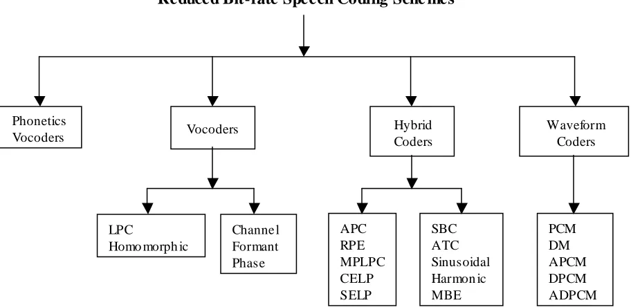
Speech coding schemes are broadly classified into four categories as illustrated in the Figure 3.1. The basic principle of these coders is to analyze the speech signal to remove the

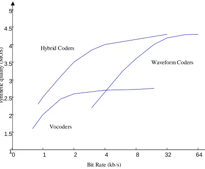
redundancies and code the non-redundant parts of the signal in perceptually acceptable manner. In the following sections only three main categories are described. The quality vs bit rate for

three main coding methods are shown in Figure 3.3. A summary of the speech coding methods, the bit-rate and mean square score (MOS) ranging from 1 to 5 are listed in the table 3.1 Generally, coding quality with MOS higher than 4 is considered as toll quality, between 3.5 and

4 as communication quality, between 3 and 3.5 as professional quality, and below 3 as synthetic quality [17].

3.3. Waveform coder:

Waveform coders attempt to code the exact shape of the speech signal waveform, without considering in detail the nature of human speech production and speech perception. Waveform

coders are the most useful in applications that require the successful coding of both speech and nonspeech signals. In the public switched and telephone network (PSTN), for example signaling

Vocoders Hybrid Coders

Waveform Coders

LPC

Homo morph ic

Channe l Formant Phase APC RPE MPLPC CELP SELP SBC ATC Sinusoidal Harmon ic MBE PCM DM APCM DPCM ADPCM Phonetics Vocoders

Reduced Bit-rate Speech Coding Sche mes

Figure 3.1 Classification of speech coding schemes

Application

Rate

(kbps) MOS Standard Algorithm Year

64 ITU-G.711 µ-law or A-law PCM 1972

32 ITU-G.721 ADPCM 1984

16-40 ITU-G.726 VBR-ADPCM 1991

Landline Telephone

16-40 ITU-G.727 Embedded-ADPCM 1991

48-64 ITU-G.722 Split-band ADPCM 1988

Tele conferencing

16 ITU-G.728 Low-delay CELP 1992

Digital Cellular 13 12.2 7.9 6.5 8.0 4.75-12.2 1-8

GSM-Full rate

GSM-EFR TIA IS-54 CDMA-TIA IS-96 GSM-Half rate ITU-G.729 GSM-AMR LTP_RPE ACELP VSELP Qualcomm CELP VSELP CSA-CELP ACELP 1989 1995 1991 1991 1994 1995 1998

5.3-6.3 ITU-G723.1 MPLPC, CELP 1996

Multimedia

2.0-18.2 ISO-MPEG-4 HVXC, CELP 1998

4.15 INMARSAT-M IMBE 1990

Satellite telephony

3.6 IMMARSAT Mini-M AMBE 1995

DDVPC FS1015 LPC-10e 1984

DDVPC MELP MELP 1996

DDVPC FS1016 CELP 1989

Secure communications

DDVPC CVSD CVSD

0 1 2 4 8 32 64 1

1.5 2 2.5 3 3.5 4 4.5 5

Bit Rate (kb/s)

sy

n

th

et

ic

q

u

ality

(M

O

S

)

Waveform Coders

Vocoders Hybrid Coders

Figure 3.2 Quality comparison of speech coding schemes

3.3.1 Pulse Code Modulation

In pulse code modulation (PCM) coding the speech signal is represented by as series of quantized samples. Since the these are memoryless coding algorithms, each sample of the signal

3.3.1a. Uniform PCM:

Uniform PCM is the name given to quantization algorithms in which reconstruction levels are uniformly distributed between Smax and Smin. The advantage of uniform PCM is that

quantization error power is independent of signal power; high-power signals are quantized with

the same resolution as low-power signals. Invariant power is considered desirable in many digital audio applications, so 16-bit uniform PCM is standard coding scheme in digital audio.

The error power and SNR of uniform PCM coder vary with bit rate in a simple fashion.

Suppose that a signal is quantized using B bits per sample. Then, the quantization step size ∆ is

1 2 min max − − = ∆ B S S 3.1

Assuming that quantization error are uniformly distributed between ∆/2 and -∆/2, the

quantization error power is

[

]

E 3.2

B S

S ) 6

( log 20

constant+ _{10 max} − _min −

≈ 3.3

3.1b Companded PCM

logarithm function prior to quantization and being expanded by the exponential function after

decoding

0 0.1 0.2 0.3 0.4 0.5 0.6 0.7 0.8 0.9 1 0

0.1 0.2 0.3 0.4 0.5 0.6 0.7 0.8 0.9 1

µ=25 6

µ=64

µ=16

µ=4

µ=1

µ=0

Inp ut signa l s(n)

O

ut

p

ut

S

ign

a

l

t(

n)

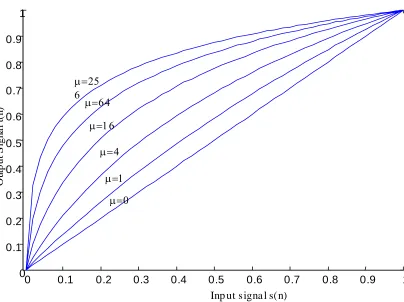
Figure 3.3 µ-law companding function µ=0 ,4,16…256.

Lo g| | Q[ ]

SIGN[ ]

x(n) y(n)

c(n) encoder

) ( ˆ n y

encoder SIGN[ ]

c(n)

It can be shown that, if small values of s(n) are more likely than large values, expected error power is minimized by companding function that results in a higher density of reconstruction

levels at low signal levels than at high signal levels. A typical example of µ-law

companding function [2] (Fig 3.3), which is given by )

( ˆ k x

)] ( [ )

(n F x n

y = 3.4

. [ ( )] ]

1 log[

) ( 1 log

max

max sign x n

x n x

x

µ µ

+ ⎥ ⎦ ⎤ ⎢

⎣ ⎡

+

= 3.5

Where µ is typically varies between 0 and 256 and determines the amount of nonlinear

compression applied.

3.4. Voice vocoders:

In contrast to waveform coders voice vocoders consider the details in the nature of human

speech. In their principles, there is no attempt to match the exact shape of the signal waveform. It consists of an analyzer and synthesizer. The analyzer attempts to estimate the model parameters,

which represent the original signal, and then transmit them. The speech is synthesized using the parameters to produce an often crude and synthetic constructed speech signal. Since the synthesized signal is either crude or distorted, SNR is not a good measure of the speech quality,

vocoders are 2.4 kbit/sec LPC-10[13], RELP [22], Homomorphic vocoder [23] [24], and the

channel and the formant vocoder [25].

The complete description of linear prediction including LPC vocoder and MBE is presented in the chapter 4.

3.5. Hybrid coders:

To overcome the disadvantages of waveform coders and voice vocoders, hybrid coding methods have been developed which incorporate each of the advantages offered by the above schemes. Hybrid coders are broadly classified into two sub-categories:

• Frequency domain hybrid coders:

• Time domain hybrid coders:

3.5.1 Time domain hybrid coders:

These can be classified as analysis by synthesis (AbS) LPC, in which the system

parameters are determined by linear prediction and the excitation sequence is determined by a closed loop or open loop optimization. The optimization process determines an excitation

sequence, which minimizes a measure of the weighted difference between the input speech and the coded speech. The weighting or filtering function is chosen such that the coder is “optimized” for the human ear. The most commonly used excitation model used for AbS LPC

are: the multi pulse, regular pulse excitation, vector or code excitation. Since these methods combines the features of model-based vocoders, by representing the formant and the pitch

structure of the AbS model and the complete explanation relating the component in the block

diagram are presented in the following subsections

3.5.1.1 The Basis LPC Analysis by Synthesis Model:

The basic structure of an AbS model coding system is illustrated in Figure 3.5. It consists

by the following three components (1) Time-Varying filter

(2) Excitation signal

(3) Perceptually based minimization procedure

The model requires frequent updating of the parameters to yield a good match to the

original, the analysis procedure of the system is carried out in blocks, i.e., the input speech is partitioned into suitable blocks of samples. The length and update of the analysis block or frame

determines the bit rate or capacity of the coding schemes.

W(z) s(n)

Perceptual Weighting

Min imize Error LPC Excitat ion

Vectors

1/A(z) LPC _Synthesis

W(z) Perceptual Weighting

(n) sˆ

(n) sˆ_w

+

-

Get specified codevector LPC Excitat ion

Vectors

1/A(z) LPC _Synthesis u(n)

(n) sˆ

(a) (b)

Figure 3.5 General structure of an LPC-AS coder (a) and decoder (b). LPC filter A(z) and perceptual weighting filter W(z) are chosen open-loop, then the excitation vector u(n) is

3.5.1.1(a) Short-Term Prediction filter

In Basic LPC model is also termed as Short-time Predictor (STP), which is illustrated in Figure 3.5. The complete description of LPC model and estimation of the filter coefficients will be discussed in chapter 4. The STP models the short-time correlation in the speech signal

(spectral envelope), and has the form given by

∑

where ai, are the STP (or LPC) coefficients and p is the filter. Most of the zeros in A(z)

represents the vocal tract or formant frequencies. Then, the number of LPC coefficients (p) depends on the signal bandwidth. Since each pair of complex-conjugate poles represents one formant frequency and since there is on average, one formant frequency per 1 kHz, p is typically

equal to 2BW (in kHz) + (2 to 4). Thus, for a 4 kHz speech signal, a 10th-12th order LPC model would be used.

3.5.1.1(b) Long Term Prediction Filter:

The LTP model the long – term correlation in the speech (fine spectral structure), and has

the form given by

∑

P ( )

1 1 ) ( 1 3.7

Where D is a pointer to long-term correlation which usually corresponds to the pitch period or its multiples and bi are the LTP gain coefficients. The process to estimation of parameters is

i.e., 2-tap taps. There is no specific limitation on the order of filters; sometimes the LTP filter is

omitted, as in MPLPC.

3.5.1.1(c) Perceptually based minimization procedure

The Abs-LPC coder of Figure 3.4 minimizes the error between the original signal s(n)

and the synthesized signal according to a suitable error criterion by varying the excitation

signal and the STP and LTP filters. This is achieved via a sequential procedure. First, the time-varying filter parameters are determined, and then the excitation is optimized.

) ( ˆ n s

The optimization criterion used for both procedures is the commonly used mean squared error criterion, which is simple and gives an adequate performance. However, at low bit rates, with one or less bit per sample, thus it is very difficult to match the original signal.

Consequently, the mean squared error criterion is meaningful but not sufficient. An error criterion, which is near to human perception, is necessary. Although much research on auditory

perception is in progress, no satisfactory error criterion has yet emerged. In the meantime, however, a popular but not totally satisfactory method is use of weighting filter in AbS-LPC schemes. The weighting filter is given by

) / ( ) ( ) ( γ z A z A z

W = 3.8

0 1

1 1

1

1 ≤ ≤

− − =

∑

∑

A typical plot of its frequency response is shown in Figure 3.6. The factor γ does not alter

the center formant frequencies, but just expands the bandwidth of the formants by ∆f given by

γ πs ln

f

f =−

where fs is the sampling frequency. As can be seen from Figure 3.5, the weighting filter

de-emphasis the frequency regions corresponding to the formants as determined by the LPC analysis. By allowing larger distortion in the formant regions, noise that is more subjectively

disturbing in the formant nulls can be reduced. The amount of de-emphasis controlled by γ. Most

suitable value of γ is usually around 0.8-0.9

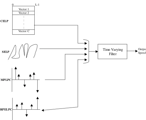
3.5.1.1(d) Excitation Signal

The excitation signal is an input to AbS-LPC model and its generation procedure is an

important block of the model shown in figure 3.4. This is because excitation signals represent the structure of the residual signal, which is not represented by the time-varying filters (STP and

LTP). e.g., speech signals with correlation greater than the LTP delay range, and also the structure that is random in that they cannot be efficiently modeled by deterministic methods. The excitation can be of any form, and can be modeled by the Equation 3.11. A block diagram of an

AbS-LPC with different excitation types is shown in Figure 3.7.

i i i g X

U = 3.11

where Ui is a L-dimensional ith excitaion vector, xi represents M×L dimensional ‘shape’ vectors

SELP

MPLPC

RPELPC

Vector 1 Vector 2

: : : : Vector C 0 L-1

CELP

Time Varying Filter

Output Speech

Figure 3.6 Generalised block diagram of AbS-LPC coder with different excitation types

3.5.2.1 Code Excited Linear Predictive coding

In the codebook excitation (CELP) [26], the excitation vector chosen from a set of pre-stored collection of C possible stochastic sequences with an associated scaling or gain vector.

Although the scaling vector is usually just a scalar factor, it can be more than one, scaling the excitation vector elements in various parts of the vector accurately. Thus to retain the generality

optimum gains gk1…….., gkM for each index k, 1≤k≤c. Thus for codebook excitation, the

excitation U can be written as

i i i g X

U = k =1_KK,C 3.12

where [ 1 , ]

i kM i

k

k g g

g = _KK i=1_KK,L/M

otherwise

1 , , 1 , 0 for

0

− =

⎪⎩ ⎪ ⎨ ⎧

= c j L

X

k j k

K

In the AbS procedure the C possible c sequences are systematically passed through the

combined sythesis filter, Hc(Z), and the vector that produces the lowest error is the desired

sequence. Since the set of sequences are present at both the encoder and decoder, only index k, to

the codebook is required to be transmitted. Therefore, less than 1 bit/sample is possible.

As the codebook is of finite dimension, it must be populated with representative vectors of the excitation to be encoded. In Atal’s original proposal, unit variance white Gaussian random

numbers were used. This choice of population was reported to give very good results, and was partly due to the fact that pdf of the prediction error samples, produced by inversing filtering the

speech through both STP and LTP filters, is very close to Gaussian. Another popular choice of codebook entries is center clipped Gaussian vectors, which both reduce complexity and improve performance.

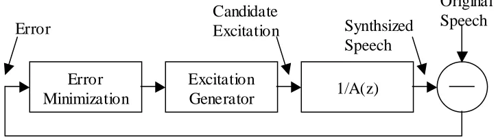
3.5.2.2 Multipulse-Excited LPC

speech over the current analysis frame (typically 5ms long). Figure 3.8 illustrates the multipulse

analysis loop.

To determine a pulse location and amplitude the excitation generator produces an excitation sequence for each possible pulse location in the analysis frame. These candidate

excitations are passed through the synthesis filter, and the MSE between the synthesised and original speech measured. The optimum pulse amplitude is obtained by minimising the MSE at

each candidate pulse position. The candidate position and amplitude that minimises the MSE is chosen, and the procedure is repeated for the desired number of pulses.

Error Minimization

Excitation

Generator 1/A(z)

Error

Candidate

Excitation Synthsized Speech

Original Speech

Figure 3.&: Multipulse-Excitation Encoder

This technique is a form of analysis by synthesis or closed-loop coding, as the canditate

excitation signals are synthesised as part of the analysis procedure.

The pulse locations and amplitudes for successive pulses are found iteratively to reduce

complexity. After the optimum position and amplitude of pulse n has been chosen, the synthesised speech from this pulse is subtracted from the original speech. The result of the

subtraction is then used as the original speech for determing pulse n +1.

Multipulse coders can produce communications quality speech at bit rates of around 10

kbit/s. Typically around 4-8 pulses per 5ms analysis frame are required for communications quality speech. At bit rates below 10 kbit/s, not enough bits are available for the number of pulses required to produce an adequate excitation signal.

A low complexity development of Multipulse-Excitation is Regular Pulse Excitation (RPE) [28]. This coder only optimizes the position of the first pulse in each analysis frame, the

Chapter 4: Linear Prediction of Speech

The purpose of this chapter is to introduce and discuss basic speech coding principles and the

complete description of Linear Prediction of Speech vocoder.

4.1. Linear prediction in speech coding

The human speech production process reveals that the generation of each phoneme is characterized basically by two factors: the source excitation and the vocal tract shaping. In order

to model speech production we have to model these two factors. To understand the source characteristics, it is assumed that the source and the vocal tract model are independent [1]. The vocal tract model H(z) is excited by a discrete time glottal excitation signal u(n) to produce the

speech signal s(n). During unvoiced speech, u(n) is a flat spectrum noise source modeled by a random noise generator. On the other hand, during voiced speech, the excitation uses an estimate

of the local pitch period to set an impulse train generator that drives a glottal pulse shaping filter. The speech production process is shown in Fig. 4.1.

Speech Glottal excitation

S(n) u(n) _{Vocal tract model}

H(z)

The most powerful and general linear parametric model used to model the vocal tract is

the autoregressive moving average (ARMA) model. In this model, a speech signal s(n) is

considered to be the output of a system whose input is the excitation signal u(n). The speech sample s(n) is modeled as a linear combination of the past outputs and the present and past inputs

[7]. This relation can be expressed in the following difference equation

∑

∑

( 4.1

where G (Gain factor) and a(k) , b(l) (filter coefficients) are system parameters. Since signal s(n)

is predictable from the linear combinations of past outputs and inputs. Hence the name linear prediction is used. The transfer function of the system can be obtained by taking Z-transform on Equation 4.1 with further simplifications:

∑

∑

( 4.2

where is the z transform of the s(n) and U(z) is the z transform of u(n). clearly

H(z) is a pole-zero model or autoregressive moving average (ARMA) model. The zeros represent the nasals, while the formants in a vowel spectrum represented by the poles of H(z).

There are two special cases of this model.

∑

• When for H(z) reduces to an all-pole model, which is also known as an

autoregressive model. ,

0

= l

b 1≤l ≤q,

• When for H(z) becomes all-zero model or a_k =0, 1≤k ≤ p, moving average model.

Speech signal is a time varying acoustic pressure wave. For the purpose of analysis and

coding, it can be converted to electrical form and sampled. Speech signals are non-stationary; the characteristics of speech evolve over time. As the characteristics vary slowly, speech signals can

be approximated as stationary over short periods (in the order of a few tens of milliseconds). With this assumption all-pole model or autoregressive model is widely used for it simplicity and computational efficiency. It models sounds such as vowels well enough. The zeros arise only in

nasals and in unvoiced sounds like fricatives. Poles approximately model the voiced sounds. Moreover, it is easy to solve for an all-pole model. In order to solve for a pole-zero model, it is

necessary to solve a set of nonlinear equations, but in the case of an all-pole model only a set of linear equations needs to be solved.

The transfer function of an all-pole model is

∑

= − −

= _p

k

k kz

a G z

H

1

1 )

( 4.3

Actually an all-pole model is a good approximation of the pole-zero model. According to

[1], any causal rational system H(z) can be decomposed as

) ( ) ( ' )

(z G Hmin z H z

where, G’ is the gain factor, is the transfer function of a minimum phase filter and

is the transfer function of an all-pass filter. ) ( min z H ) (z H_ap

Now, the minimum phase component can be expressed as an all-pole system:

∑

where I is theoretically infinite but practically can take a value of a relatively small integer. The all-pass component contributes only to the phase. Therefore, the pole-zero model can be

estimated by an all-pole model.

If the gain factor G = 1, then from Equation 4.5 the transfer function becomes

∑

( 4.6

) ( 1 z A =

where the polynomial

(

∑

)

The error signal e(n) is the difference between the input speech and the estimated speech.

Thus the following relation holds:

∑

=

− −

= P

k

ks n k

a n

s n e

1

) ( )

( )

( 4.7

In the z-domain it is equivalent to

) ( ) ( )

(z S z A z

E = 4.8

Now, the whole model can be decomposed into the following parts, the analysis part and

the synthesis part (see Figure 4.2)

error signal speech signal

e(n)

s(n) _{Analysis filter}

A(z)

error signal speech signal

e(n) _{Synthesis Filter} s(n)

1/A(z)

Figure 4.2 LP Analysis and synthesis model

The analysis part analyzes the speech signal and produces the error signal. The synthesis part takes the error signal as an input. The input is filtered by the synthesis filter 1/A(z), and the output is the speech signal. The error signal e(n) is sometimes called residual signal or excitation

exactly the inverse of the analysis filter, the synthesized speech signal will not be the same as

original signal. To differentiate between the two signals, we use the notation s for the synthesized speech signal.

In general excitation signal for the synthesized filter either error signal or periodic

impulse train/white noise input.

4.1.1 Role of Windows

Speech is a time varying signal, and some variations are random. Usually during slow speech, the vocal tract shape and excitation type do not change in 200 ms. But phonemes have an

average duration of 80 ms. Most changes occur more frequently than the 200 ms time interval [30]. Signal analysis assumes that the properties of a signal usually change relatively slowly with

time. This allows for short-term analysis of a signal. The signal is divided into successive segments, analysis is done on these segments, and some dynamic parameters are extracted. The signal s(n) is multiplied by a fixed length analysis windoww(n) to extract a particular segment at

a time. This is called windowing. Choosing the right shape of window is very important, because it allows different samples to be weighted differently. The simplest analysis window is a

rectangular window of length Nw:

⎩ ⎨ ⎧ =

0 , 1 ) (n

w

otherwise N

n w 1,

0≤ ≤ −

4.9

A rectangular window has an abrupt discontinuity at the edge in the time domain. As a

window without abrupt discontinuities in the time domain. This corresponds to low side lobes of

the windows in the frequency domain. The Hamming window of Equation 4.10, used in this research, is a tapered window. It is actually a raised cosine function:

⎪⎩ ⎪ ⎨ ⎧ − ∏ − = , 0 ), 1 2 cos( 46 . 0 54 . 0 )

( Nw

n n

w

otherwise N

n _w 1,

0≤ ≤ −

4.10

There are other types of tapered windows, such as the Hanning, Blackman, Kaiser and the Bartlett window. A window can also be hybrid. For example, in GSM 06.90, the analysis

window consists of two halves of the Hamming windows with different sizes [31].

4.1.2 LP coefficient computation

There are two widely used methods for estimating LP coefficients. Both methods choose the short-term filter coefficients (LP coefficients) {ak}in such a way that the residual energy (the

energy in the error signal) is minimized. The classical least square technique is used for that purpose. In each of the two formulations predictor coefficients are computed by solving a set of p equations with p unknowns. These equations are

), ( ) ( 1 i R k i R a p k

k − =−

∑

=

1≤i≤ p for autocorrelation 4.11

where

∑

−

=

−

= 1 ( ) ( )

) ( w N i n w w n s n i

s i

R w is the windowed speech signal sw(n)=w(n)s(n)

i p k ki k a ₀ 1 ϕ ϕ =−

∑

where

∑

ik s n i s n k

ϕ

There exits several standard methods to solve the above linear equations eg., the Gauss

reduction or elimination method and Crout method. But other methods like square-root or Cholesky decomposition method, needs only half of the number of operations (multiplication or

divisions) and half of the storage of the precious methods, because covariance is symmetric and semi-definite. Further reduction in storage and computation is possible in solving the auto-correlation normal Equations 4.11 because of their special form. Equation 4.11 can be expanded

in matrix form as

⎥ ⎥ ⎥ ⎥ ⎦ ⎤ ⎢ ⎢ ⎢ ⎢ ⎣ ⎡ = ⎥ ⎥ ⎥ ⎥ ⎥ ⎦ ⎤ ⎢ ⎢ ⎢ ⎢ ⎢ ⎣ ⎡ ⎥ ⎥ ⎥ ⎥ ⎦ ⎤ ⎢ ⎢ ⎢ ⎢ ⎣ ⎡ − − − − ) 3 ( ) 2 ( ) 1 ( . ) 0 ( ) 2 ( ) 1 ( ) 2 ( ) 0 ( ) 1 ( ) 1 ( ) 1 ( ) 0 ( 2 1 R R R a a a R p R p R p R R R p R R R p M M L M O M M L L 4.13

the above p × p auto-correlation matrix is symmetric and the elements along the diagonal are identical. Levinson derived an elegant recursive procedure for solving this type of equation, later formulated by Robinson. Durbin’s procedure can be specified as follows.

) 0 (

0 R

E = 4.13

1 1 1 ) 1 ( ) ( ) ( ₋ − = − ⎥ ⎦ ⎤ ⎢ ⎣ ⎡ − + −

=

∑

j i j

i R i a R i j E

k 4.14

i i

i k