by
Derek Caleb Klein
A thesis
submitted in partial fulfillment of the requirements for the degree of Master of Science in Computer Engineering
Boise State University
DEFENSE COMMITTEE AND FINAL READING APPROVALS
of the thesis submitted by
Derek Klein
Thesis Title: Non-Blocking Hardware Coding for Embedded Systems
Date of Final Oral Examination: 16 March 2011
The following individuals read and discussed the thesis submitted by student Derek Klein, and they also evaluated his presentation and response to questions during the final oral examination. They found that the student passed the final oral examination, and that the thesis was satisfactory for a master’s degree and ready for any final modifications that they explicitly required.
Sin Ming Loo, Ph.D. Chair, Supervisory Committee
Thad B. Welch, Ph.D. Member, Supervisory Committee
Hao Chen, Ph.D. Member, Supervisory Committee
ACKNOWLEDGMENTS
I would like to thank my thesis advisor, Dr. Sin Ming Loo, for his guidance and
patient support throughout this process. His contribution has been essential to my
academic pursuits.
Additionally, I would like to thank those who were involved in this research: Josh
Kiepert, Jim Hall, Michael Pook, Kelsey Drake, and Ross Butler. Their significant
contributions made this research possible. I would like especially thank Josh Kiepert, Jim
Hall, and Michael Pook for their participation in the implementation of several of the
non-blocking techniques discussed in this thesis. Michael Pook deserves further thanks
for his assistance in the final editing of this thesis.
Finally, I would like to thank my family. Their love and support has made my
success in academics and life in general possible. I would like to specifically
acknowledge my brother, Daren Klein, who inspired me to go to college with his
dedication to overcoming dyslexia while learning to read. My mother deserves special
thanks for putting up with me as my teacher and mother growing up. A person could not
ask for a better mother. Thanks, mom.
This work is funded by FAA Cooperative Agreement No. 04-C-ACE-BSU and 07-C-RITE-BSU1.
1
ABSTRACT
NON-BLOCKING HARDWARE CODING
FOR EMBEDDED SYSTEMS
Derek Klein
Master of Science in Computer Engineering
Embedded Systems can be found in devices that people use every day. In the
pursuit of faster and smarter devices, more powerful processing units are needed in these
embedded systems. A key component of powerful processing units is the supporting
software. While the raw processing power of microcontroller has been continually
advancing, the improvements in the supporting software for medium scale embedded
systems have been lacking. This thesis focuses on improving the software on medium
scale systems by discussing the practical application of non-blocking coding techniques.
The basic concept of how non-blocking code improves the performance of a system is
relatively easy to understand. However, non-blocking code is considerably more
challenging to implement in practice. This thesis shows that, by utilizing some commonly
known coding techniques and practices together in a systematic manner, it is possible to
obtain practical non-blocking software on medium scale embedded systems. It was found
that under certain conditions more than 20% of the total processor time can be saved by
converting a blocking I2C driver to non-blocking. The freed processing time improved the
TABLE OF CONTENTS
ACKNOWLEDGMENTS ... iv
ABSTRACT ... v
LIST OF TABLES ... x
LIST OF FIGURES ... xi
LIST OF ABBREVIATIONS ... xiii
CHAPTER 1: INTRODUCTION ... 1
1.1 Embedded Systems ... 1
1.2 Embedded System Categories ... 3
1.3 Software for Sensor Networks ... 5
1.4 Thesis Purpose ... 6
1.5 Overview ... 7
CHAPTER 2: RESEARCH BACKGROUND ... 8
2.1 Limited Related Research ... 8
2.2 Common Coding Practice ... 9
2.2.1 Hardware Interface ... 10
2.3 Operating Systems ... 14
2.3.1 Dynamic Memory ... 15
2.3.2 Process Scheduler ... 15
2.3.3 I/O Subsystem ... 16
2.4 Scheduler ... 18
2.4.1 Superloop ... 19
2.4.2 Time Triggered ... 19
2.4.3 Cooperative ... 19
2.5 Systems without Operating System ... 20
CHAPTER 3: HARDWARE PLATFORM ... 21
3.1 Sensor Modules ... 21
3.2 Processor ... 22
3.3 Breakout Board Sensor Interface ... 22
3.4 Power ... 24
3.5 Network Communications ... 25
3.6 Data Storage ... 25
CHAPTER 4: NON-BLOCKING CODING PRACTICES... 27
4.1 Blocking Code ... 27
4.2.1 Circular Buffer ... 31
4.2.2 State Machine... 35
4.2.3 Callback Function ... 38
4.3 Example Code ... 40
4.3.1 Blocking Code Example ... 40
4.3.2 Non-Blocking Example ... 41
4.4 Appropriate Uses of Blocking Code ... 44
CHAPTER 5: NON-BLOCKING ANALISIS ... 46
5.1 I2C Hardware Driver Analysis ... 48
5.1.1 I2C Blocking Driver Description ... 49
5.1.2 I2C Non-Blocking Driver Description ... 50
5.1.3 I2C Waveform Analysis ... 52
5.1.4 I2C Throughput Analysis ... 59
5.2 UART Driver Analysis ... 62
5.2.1 UART Blocking Driver ... 63
5.2.2 UART Non-Blocking Driver ... 64
5.2.3 UART Waveform Analysis ... 65
5.2.4 UART Blocking Driver Effects on Network Throughput ... 68
6.1 Summary and Conclusions ... 71
6.2 Future Work ... 72
6.2.1 Linked List ... 72
6.2.2 SD Card Interface ... 73
LIST OF TABLES
Table 1.1: Embedded System Catagorization ... 4
Table 5.1: Non-Blocking I2C Driver Effect on Network Tasks ... 60
Table 5.1: Blocking I2C Driver Effect on Network Tasks ... 60
Table 5.3: Non-Blocking UART Driver Effect on Network Tasks ... 70
LIST OF FIGURES
Figure 2.1: ADC Reading Function ... 11
Figure 2.2: Common Main Function in Embedded Systems ... 13
Figure 3.1: Sensor Module Board ... 21
Figure 4.1: Basic Function Call Format ... 29
Figure 4.1: Circular Buffer ... 32
Figure 4.3: Generic Circular Buffer ... 35
Figure 4.4: State Machine ... 37
Figure 4.5: Callback Function... 39
Figure 4.6: Blocking Transmit Function ... 41
Figure 4.7: Non-Blocking Transmit Request ... 42
Figure 4.8: Non-Blocking Transmit Interrupt Service Routine ... 43
Figure 4.9: Non-Blocking Transmit Task ... 43
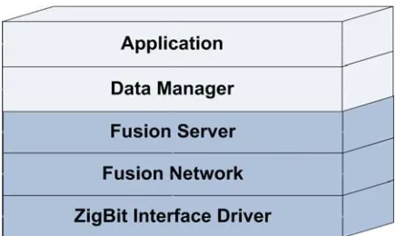
Figure 5.1: Fusion Network Software Interface ... 48
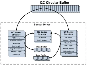
Figure 5.2: Fusion I2C Driver ... 51
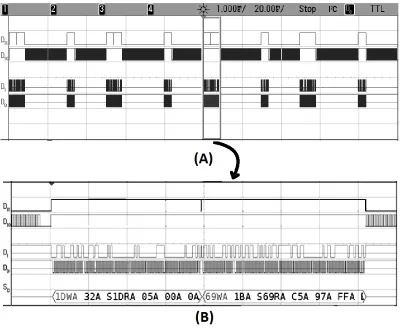
Figure 5.3: Blocking I2C Waveform ... 54
Figure 5.4: Non-Blocking I2C Waveform ... 58
Figure 5.5: I2C Effect on Network Throughput ... 62
Figure 5.6: Fusion UART Driver ... 64
Figure 5.8: Non-Blocking UART Waveform ... 68
LIST OF ABBREVIATIONS
ADC Analog-to-Digital Converter
DC Direct Current
FAA Federal Aviation Administration
FAT File Allocation Table
FIFO First In First Out
GPIO General Purpose Input/Output I/O Input/Output
I2C Inter-Integrated Circuit
ISR Interrupt Service Routine
OS Operating System
PMON Personal Monitor
SD Secure Digital
SDIO Secure Digital Input Output
SPI Serial Peripheral Interface
SRAM Static Random Access Memory
TWI Two Wire Interface
USART Universal Synchronous/Asynchronous Receiver/Transmitter USB Universal Serial Buss
CHAPTER 1: INTRODUCTION
1.1 Embedded Systems
An embedded system is an electronic system that is part of a larger system. They
can be found in devices that most people use on a daily basis. For example, embedded
systems can be found in everything from communication systems (e.g., cellular phones,
radios, etc.) to household appliances (e.g., dishwashers, refrigerators, etc.). Consumers
continue to desire faster and smarter features on our devices and appliances that require
more powerful processing units. A key component of a powerful processing unit is its
supporting software. This thesis will discuss some practical concepts that can greatly
improve the supporting software of embedded systems.
As the demands of embedded systems continue to grow, there is a need to produce
systems that are more flexible, responsive, robust, and cost effective. For example, the
original home thermostats were electromechanical systems that used bimetal strips to
simply open and close a circuit based on the ambient temperature. The user interface was
simple. Due to the demand for a better user interface and power management, today’s
thermostats have considerably more functionality. The ability to schedule different
temperature settings for different times of the day is common for thermostats currently on
the market. Some of the nicer thermostats even have touch screen interfaces. These
additional features require a more advanced embedded system with supporting software.
of more demanding applications. One area where hardware technology has made notable
increases is the processing units on embedded systems. Depending on the type of
embedded system, the processing unit is typically a microprocessor or one of many
different types of microcontrollers. The main difference between microprocessors and
microcontrollers is that microprocessors are only composed of a processing unit.
Whereas, microcontrollers include timers, memory, and specialized I/O hardware along
with the processor in a single package. The exact quantity, variety, and type of specialized
hardware on an embedded system are dependent on the application and embedded system
complexity. For all types of embedded systems, the hardware capabilities such as
available memory, processing speed, power efficiency, interface flexibility, and cost
effectiveness are continually advancing.
Advances in the supporting software are needed to take full advantage of the
improvements in hardware. Hardware and software need to work together to create the
powerful processing units in embedded systems today. Without software, the hardware
will be useless. Without hardware, the software will have no place to run. Even with the
advancements continually being made, embedded systems hardware still has limited
resources. Two of the most common limitations are memory and processor capacity. In
order to make up for these limitations, some embedded hardware (particularly
microcontrollers) has specialized devices that are designed to optimize specific tasks.
Embedded software is responsible for managing hardware resources, processing the data,
and controls how a system operates. In order to take advantage of advances in hardware,
meant by “effective use” is that the software does not add unnecessary obstacles to the
performance of the hardware. For example, blocking code (a piece of code that prevents
other processes from running while it waits for information to complete execution) in a
hardware driver might prevent another specialized piece of hardware from being fully
utilized. Development of effective non-blocking software is highly dependent on the
hardware platform. The focus of this thesis is to demonstrate a systematic way of
applying non-blocking coding practices to embedded systems in such a way as to take
full advantage of advances in embedded hardware.
1.2 Embedded System Categories
There is a wide variety of embedded systems, so it is difficult to have a set of
coding techniques apply to every type of system. The coding techniques and practices
discussed in this thesis primarily apply to a limited category of embedded systems. So it
is important to clarify what type of embedded system will be the focus of this thesis.
There are multiple ways to categorize embedded systems. Embedded systems could be
categorized based on the type of application, cost of the system, system functionality,
complexity, or hardware capabilities. The capability of the hardware is one particularly
relevant aspect for embedded software. For the purpose of this thesis, embedded systems
will be organized into three categories: small scale, medium scale, and large scale, based
on the hardware capabilities of the system. A description of these categories is provided
Table 1.1: Embedded System Catagorization Category Category Description
Small Scale Capable of supporting 1 to 2 applications. Typically on smaller 8-bit
microcontrollers that do not have enough memory to support an operating system.
Medium Scale Capable of supporting multiple applications. Typically on 32-bit and smaller
microcontrollers that do not have enough memory to support an embedded operating system.
Large scale Capable of supporting multiple applications. Typically on large microcontrollers
or microprocessors that have more than enough memory to support an embedded operating system.
For this thesis, small scale systems will be defined as being capable of supporting
only one or two applications. These systems typically have smaller 8-bit microcontrollers
with very limited memory. An example of this type of system would be a garage door
opener. A garage door opener has one application that monitors a button and sends a
signal to the garage door controls when the button is pushed. The application is
composed of two tasks: the first is monitoring the button and the second is
communicating wirelessly with the garage door controls.
Medium scale systems are capable of supporting multiple applications running at
the same time. For this thesis, medium scale systems will be defined as systems that have
enough hardware capabilities to support multiple applications but do not have the
hardware capability to practically support an operating system at the same time. A good
example of this would be the controller in a refrigerator. The control system on an
advanced refrigerator is responsible for making ice and dispensing water in addition to
controlling the temperature of two separate compartments. Each of these responsibilities
change over time, a processing unit with expansion capabilities or an operating system is
not practical.
Large scale systems are similar to general computing systems (e.g., desktop
computers) in that they are capable of supporting a wide variety of applications. They
typically have an abundance of memory to support their various functions. Large scale
systems typically have enough memory and processing speed to support a compact
operating system. A smart phone is a good example of a large scale embedded system.
1.3 Software for Sensor Networks
A sensor network is a good example of a medium scale embedded system. Like
the name suggests, the sensor network’s main purpose is to collect data from a network of
sensors. A network is composed of multiple sensor nodes. The number and variety of
sensors on each node is dependent on the sensing application. The data collected from
each sensor node is typically transmitted across a wireless network to a central location
for processing. So, with each sensor node, there are multiple applications that often need
to operate at the same time. The data collection itself is often broken up into multiple
tasks. The drivers for the interfacing hardware, the initial processing of the data, and
scheduling the intervals for collecting data are just a few of the more common tasks that
are directly used to collect the sensor data. In addition to collecting sensor data,
transmitting the data across the network can involve multiple tasks. First, there is the
driver for interfacing with the network radio. Second, if the system needs to be able to
maintained by a task. Occasionally, the data is stored locally in addition to being
transmitted. Sensor networks are typically designed to continuously monitor the subject
of interest. Consequently, all of sensor node's tasks need to continuously run alongside
each other. If one of the tasks is prevented from performing its duties, the entire system
could be negatively affected. One solution to such a problem is to upgrade the system
scale and include an operating system. However, since the general idea is to have a sensor
network composed of a large number of nodes, it is desirable to keep each node as cost
effective as possible. Thus, large scale embedded systems are impracticable for the
typical sensor network.
1.4 Thesis Purpose
This thesis demonstrates coding techniques for non-blocking software on medium
scale embedded systems. The scientific community has focused on establishing coding
techniques and practices for large scale embedded systems. However, there is still a need
for medium scale embedded systems in research and industry. Industry typically relies on
the experience of designers to produce a quality non-blocking code. However, differences
in the abilities of designers can lead to a variety of approaches that results in software that
is difficult to maintain and port from one platform to another. A formulated systematic
approach can help establish more consistent coding practices that are easier to port across
platforms. By examining how the different aspects of non-blocking coding techniques
work together, a systematic approach of applying these techniques to medium scale
1.5 Overview
The following chapters will discuss many of the aspects of non-blocking coding
practices as they apply to medium scale embedded systems. This discussion will focus on
sensor networks in particular. Chapter 2 will cover the background of embedded system
software and how it relates to this thesis. Chapter 3 will provide a description of the
sensor node hardware used for this research. Chapter 4 will discuss several coding
techniques that are used in developing non-blocking code. Chapter 5 provides analysis
for two non-blocking coding examples. Finally, the conclusions and possible future work
CHAPTER 2: RESEARCH BACKGROUND
2.1 Limited Related Research
There is a significant amount of research focused on improving software in
embedded systems. Unfortunately, most of the research is dedicated to large scale
embedded systems. Over the years, there have been a lot of operating systems based
software research developed on general computing systems (e.g., desktop computers).
Presently, the hardware on large scale embedded systems has advanced to the point where
an operating system is a practical option. Embedded software research is primarily
focused on applying the operating system principle developed on general computing
systems to large scale embedded systems. Consequently, there is a lot of potential with
research focused on large scale embedded systems. Unfortunately, this research based on
operating systems does not really apply to the medium scale embedded systems that are
the focus of this thesis. Medium scale systems typically do not have the memory
resources to support an embedded operating system. In addition to this, medium scale
systems tend to be very specialized. This specialization makes applying generalized
operating systems a challenging option. So developing a generic operating system that
covers medium scale embedded systems is not practical.
To date, general coding guidelines for coding practices in medium scale
embedded systems have not been established in the industry. There is very little published
that relates to medium scale systems have to do with schedulers [1]. Although schedulers
are a crucial component of embedded systems with or without an operating system, they
are not the only important aspect to which coding guidelines could be applied. With the
wide variety of specialized medium scale embedded systems, it is also difficult to
establish coding techniques that apply directly to every application. Consequently, coding
techniques for these types of systems have been gained primarily through personal
experience and instruction. Some of these techniques are discussed in Section 2.2. With
such a limited amount of research for medium scale systems, there is still a need to
develop effective coding practices that are not based on an operating system. This thesis
attempts to demonstrate techniques and methods that will produce effective non-blocking
software that can be applied to these types of systems.
2.2 Common Coding Practice
Since there is limited published research on coding practices in embedded
systems, most coding practices are based on experience. This experience typically
consists of problems encountered and instruction from experienced colleagues.
Embedded system designers often have different experience based on the variety of
hardware platforms on which they have worked. Consequently, coding practices can vary
quite a bit among designers. In spite of this, certain common practices have been
developed. Most of the practices stem from the need to use a common framework for
development and the clear benefits of each technique/practice. These common practices
interfacing with hardware, and the main system loop.
2.2.1 Hardware Interface
The main purpose for most embedded systems is interfacing with hardware
whether it is a sensor, control device (e.g., DC motor, Solenoid etc.), or communication
(e.g., UART, wireless transceiver, etc.). There are many different approaches taken to
interfacing with hardware. Three of the more notable approaches are polling, waiting, and
interrupting.
Polling can be used by itself or in concert with the other two approaches. As a
result, polling is a little bit harder to distinguish from the others. The basic idea of polling
is that the condition of some hardware is periodically checked. When polling is used by
itself, a task/application that is accessing the hardware will periodically check the status
registers associated with the hardware. If the status registers indicate that the hardware is
ready, the task will perform the related operations and return control back to the
scheduler. If the status registers indicate that the hardware is not ready, then the task will
return the control back to the scheduler without performing the related action. The
problem with polling by itself is that there is high probability of missing a hardware
action while another task is being handled.
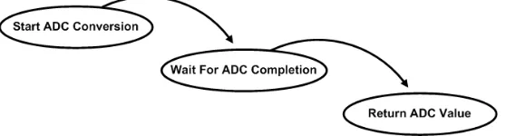
Another common method is the wait-poll approach. When a hardware interface
function is called by an application, the function waits until the hardware action is
complete. For example, suppose an application needs to access the value of an
method is shown in Figure 1.1. At the beginning of the function, the hardware to starts an
ADC read. The function then waits for the ADC hardware to finish. This usually involves
polling a flag in a hardware register. After the ADC finishes, the function returns the
result from the ADC register. The advantage of this method of interfacing with the
hardware is that it is very simple to implement. Unfortunately, this blocks other
potentially useful work from being completed. Processor cycles are wasted during each
wait.
Figure 2.1: ADC Reading Function
Another approach to interfacing with hardware is through the use of interrupts.
Most of the hardware interfaces on microcontrollers have interrupts that are triggered
when either a monitored device changes state or a particular hardware task completes.
When an interrupt occurs, the microcontroller will pause the current process and execute
an interrupt service routine (ISR). The ISR will perform the operations for the hardware
that triggered the interrupt. It is important to keep an ISR short, because it will prevent
other lower level interrupts from occurring. So, it is generally not a good idea to call
functions from inside an ISR (especially I/O functions such as "printf"). Sometimes, in
order to keep the entire ISR short, only the absolutely necessary operations are performed
ISR. Interrupts are important to non-blocking systems as they give an effective alternative
to the wait-poll method. Unfortunately, interfacing with an interrupt is not always trivial.
When using an interrupt, it is necessary to figure out how much of a given process must
occur in the interrupt. Typically, for an interrupt to be used effectively, it has to control a
state machine. Sometimes this is done indirectly through the use of flags. Other times, the
interrupt service routine has to modify the state machine directly. One must carefully
balance the time critical nature of a given process against the need to keep ISR's as short
as possible.
2.2.2 Main Function
One of the most common practices in medium scale embedded systems is related
to the centralized control of the main function. The main by default is the first function
executed upon startup. One thing that medium embedded systems have in common is that
there are a variety of settings that have to be initialized at start up. Additionally, there are
typically a few tasks that continually run. Consequently, a typical main will have an
initialization routine followed by a while loop like the example in Figure 2.2. Notice that
the initialization routines are executed first and are responsible for setting all of the
hardware registers to the appropriate values for the applications involved. The actual
organization of the initialization sequence will depend on the hardware platform and the
designer’s preferences. The next piece of code to be executed is the main loop. The main
while loop is the core of a typical embedded system. It is responsible for continually
updating the tasks for the different applications running on the system. While there are
most common. This scheduling routine is commonly referred to as the super loop (an
infinite loop). There are a couple of reasons this method is commonly used. The first is
that it is simple. Each task will eventually get its turn to run as long as none of the tasks
block indefinitely. The other reason is that embedded systems operate continually. The
main while loop will continue to execute the application tasks indefinitely as long as
there is not a catastrophic failure.
main() {
Init_sensor1(); // setup i/o register and calibration values Init_uart(); // setup baud rate and port
While() {
Interface_sensor1(); //get data from sensor1 Interface_uart(); // output collected data to uart and
// send status message }
}
Figure 2.2: Common Main Function in Embedded Systems
The potential problem with this method is that, if one task blocks for too long,
then the other processes will be losing processing time. So, it is important to minimize
the execution length of each task. Most designers are aware of this potential problem.
Unfortunately, the effective ways to implement non-blocking techniques covered in this
thesis are not universally understood. Consequently, blocking techniques are still
commonly used in these types of embedded systems. For example, it is still common to
when accessing hardware that has a more defined communication length (e.g., an I2C
read or write). Many of the problems from blocking code will not create a problem until
the hardware platform is pushed to its limits, such as when the processing speed is barely
fast enough to execute all of the tasks in time. Another situation were a system is pushed
to its limits is when the particular piece of code is continually needing to be processed.
On the other hand, systems that are not pushed to their limits do not always suffer the
same detrimental effects from blocking software. Consequently, the individual designers
still frequently use blocking calls in certain situations based on their experience.
2.3 Operating Systems
Operating systems are composed of multiple aspects and components that make
them hard to define. One way of viewing an operating system is as a resource allocator
[2]. In other words, an operating system is designed to manage the data, processes, and
hardware. The purpose of an operating system is to create an easy-to-use interface that
effectively uses the hardware. Operating systems have been around for some time in
general computing systems. Consequently, most of the aspects of operating systems have
been well established. The operating system program itself is referred to as a kernel. A
kernel is a standalone process that directly controls all of the aspects of the operating
systems. A few of the more notable aspects that the kernel is responsible for managing are
dynamic memory, process scheduling, and I/O subsystem. The fact that operating systems
have been well defined and provide easy portability makes them an attractive option for
2.3.1 Dynamic Memory
Memory usage is a problem faced by all computing systems. In any system, there
is a limited amount of memory available. Processes can require various amounts of
memory at different times during their given tasks. An operating system minimizes the
amount of memory consumed by dynamically allocating memory. By dynamically
allocating memory when it is needed, memory can be shared and re-use by multiple
processes. So, when one process is finished using a piece of memory, it becomes
available for another process.
2.3.2 Process Scheduler
The primary function of an operating system is scheduling. An operating system
has multiple schedulers each with a unique purpose. However, the most commonly
referred to scheduler (referred to hereafter as the process scheduler) is responsible for
allocating processing time for the different processes. A process, in its essence, is simply
a task that is being executed. Furthermore, the execution of a process must progress in a
sequential fashion [2]. The operating system keeps track of a process through a process
control block. The process control block holds all the information pertaining to the
process such as process state, memory information, program counter, and all other
relevant information.
The typical embedded computing system can only run one process at a time. So
the different processes have to take turns using the processor. When processes are
of the next process is loaded. This is known as context switching. Depending on the
system, a considerable amount of processing time can be spent on context switching.
Sometimes, a process is divided up into multiple smaller light-weight processes known as
threads. Threads take turns using the processor just like processes. However, multiple
threads are part of the same process, so they can be switched out with less overhead since
they share much of the same information. All of the switching between processes and
threads is controlled by the process scheduler.
There are a multitude of scheduling algorithms to accomplish context switching,
some of which will be discussed in greater detail in Section 2.4. All of them have the
basic idea of minimizing wasted clock cycles while still remaining fair to all of the
processes and threads. So, when a process or thread is idle, it is switched out for another
in the scheduler’s ready queue. Furthermore, when a process is waiting for I/O, it is
rotated out of the scheduler’s ready queue into a waiting queue.
One advantage of operating systems is that a blocking code does not actually
block. This accomplished by rotating idle processes out of the ready queue into a waiting
queue [2]. Thus, designers are able to write simpler codes without the concern that one
process will block another on the system. This is another reason why the wait-poll I/O
access technique described in Section 2.2.1 is a common practice in embedded
applications without operating systems.
2.3.3 I/O Subsystem
hardware. The purpose of the I/O subsystem is instrumental in achieving the goals of the
operating system as a whole. First, the I/O subsystem provides a standardized interface
for the applications. The standardized interface significantly increases the portability of
applications between hardware systems as well as the extendibility of the hardware
interfaces. Consequently, additional hardware can be easily integrated into the system by
creating device drivers that follow a standard interface. “The purpose of the device driver
layer is to hide the differences among device controllers from the I/O subsystem of the
kernel” [2]. The second goal of the I/O subsystem is to optimize access to the hardware.
What is meant by "optimizing" is to reduce that amount of resources spent on accessing
the I/O hardware, which is accomplished through scheduling and buffering. The exact
approach and method for scheduling and buffering are different for each operating
system. However, the main concepts remain the same.
With multiple processes running on a system, there are occasions where two or
more processes will need to access a particular piece of hardware at the same time. Since
both systems cannot have access to the hardware at the same time, the I/O scheduler is
responsible for scheduling their access to the hardware. I/O system calls that are not
immediately processed are placed on a queue until the I/O is free. The general concept for
the I/O scheduler is to organize the system calls in a way that reduces the overall wait
time while still treating each process fairly [2].
Buffering is another way in which the effectiveness of interfacing with I/O
hardware is improved. A couple of the problems that buffering helps resolve in embedded
between an application running on the main processor and an I/O port or between two
different I/O ports. With the different speeds, the faster device will have to wait for the
slower device. By storing the data temporarily in a buffer, the faster device is free to
perform other tasks and then transmit the data in bursts. Buffering is also used to adapt
devices that have different data-transfer sizes. Data is often transmitted in segments
called packets. When communicating across a medium that only supports smaller packet
sizes, the larger packets have to be broken down and then recombined on the other end.
Buffers help facilitate the breaking down and recombination of the packet by providing a
place to store the smaller packets until all the components of the larger packet have been
transmitted.
2.4 Scheduler
As mentioned in Section 2.2.2, there are a variety of scheduling approaches. This
section will discuss how each of these approaches manages access to the processor. A
process scheduler is necessary for any system with more than one process operating at the
same time. This is true for embedded systems with or without an operating system.
Because process schedulers play such a significant role in multitasking systems, it is
possible to find published research covering a wide variety of scheduling methods. Some
research that is of particular interest to this thesis is found in [1]. This research covers
scheduling methods that can be directly applied to embedded devices without an
operating system. The three scheduling methods discussed are Superloop, time triggered,
2.4.1 Superloop
The Superloop is one of the most simple and commonly used schedulers in
embedded systems. In fact, this is the same scheduling method described in Section 2.2.2.
A Superloop, like its name suggests, is simply an infinite loop through all of the tasks of
the system in the order specified by the designer. Scalability is easy since a task is simply
added to the while loop in the necessary order. The primary drawback is responsiveness
and reliability. Embedded systems often have time-critical components. The Superloop
does not have the ability of to accurately schedule a period for each task.
2.4.2 Time Triggered
The Time Triggered scheduler uses a timer interrupt to determine when each task
is called. Since a timer is used for each task, this is not a very scalable scheduler system.
As a result, Time Triggered schedulers are not commonly used in embedded systems.
2.4.3 Cooperative
A Cooperative scheduler is essentially a combination of the two previously
discussed schedulers. One timer is set to interrupt at a regular interval, which will be the
minimum time resolution for the different tasks. Each task is then assigned a period that
is a multiple of the minimum resolution of the interrupt interval. A function is then
constantly called to update the interrupt count for each task and run tasks that have
reached their interrupt period. This results in a scheduler that has the scalability of the
Superloop with the timing reliability of the Time Triggered scheduler. This is a
without its limitations. It is still important that the task calls in a cooperative scheduler
are short. If one task blocks longer than one timer interrupt period, a time-critical task
might be missed.
2.5 Systems without Operating System
While operating systems' overhead make them impractical for a significant
portion of embedded systems, there are concepts that can still be applied to embedded
systems without a full operating system. A couple of concepts that are particularly useful
are buffering and storing process state information. Although the implementation is
different (and can be difficult) without an operating system, buffering I/O data is still just
as relevant. An embedded system still has to deal with different transfer rates and data
packet sizes with or without an operating system. A key aspect of an operating system
that prevents a process from blocking is its ability to store the process state into a process
control block. Likewise, any non-blocking system has to have the ability to store the
state of a process so another process can have its turn on the processor. Without an
operating system, the responsibility of saving its state falls to each individual process.
By applying these concepts to some of the existing coding practices and
scheduling techniques, an embedded system can still make effective use of the hardware
without an operating system. However, the implementation of these concepts without the
use of an operating system can be quite a challenge. It is the goal of this thesis to
demonstrate a generic and systematic way to accomplish this task and thereby reduce the
CHAPTER 3: HARDWARE PLATFORM
3.1 Sensor Modules
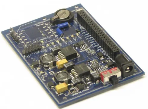
The platform used to implement the non-blocking coding techniques discussed in
this thesis is the Fusion board shown in Figure 3.1. The Fusion board was developed by
the Hartman Systems Integration Laboratory at Boise State University to replace the old
PMON board [3, 4]. Each Fusion board can be used as a single sensor collecting device,
or it can be combined with multiple Fusion sensor nodes to form a sensor network. The
Fusion board has been designed to increase performance while maintaining the flexibility
of the older PMON modules [3]. The fusion module takes advantage of the improved
hardware capabilities developed over the past few years.
3.2 Processor
Many sensor networks used in embedded applications in particular require a
flexible microcontroller with plenty of memory. The ATMEL microcontroller
AT32UC3A3256S, a 32-bit microcontroller, was chosen for the sensor modules because
of its ability to meet these requirements [5]. With 256 kbytes flash and 64 kbytes
high-speed SRAM, this microcontroller has plenty of memory to work with. Additionally, the
96 DMIPS and 66MHz processing unit found in this microcontroller is significantly
faster than the PMON’s 8-bit microcontroller PIC18F8722 [6].
This microcontroller also has a wide variety of hardware communication modules
that make it ideal for a flexible system. It has one multimedia secure digital card
communication port for storing data to removable media. Also, a high-speed universal
serial bus (USB) module is available for data transmission with a computer. An eight
channel 10-bit analog to digital converter is available for interfacing with analog sensors.
Additionally, there are two SPI modules with the capability of being set as a master or a
slave. Each SPI module has 4 chip select signals allowing for communication with 8
devices across the two ports. There are also two TWI modules that are capable of
communicating using the I2C protocol. Finally, there are also four USART modules that
are available on the microcontroller.
3.3 Breakout Board Sensor Interface
The greatest asset of the PMON modules is their flexible sensor interface [3]. In
breakout board attached to the main board through a header. This allows different
communication protocols to be used for different applications without redesigning the
entire system. Each application has a unique breakout board that is designed to
communicate to the microcontroller through the header. A variety of communication
protocols are routed to the header to maximize options for different sensor applications.
One of the most common sensor communication protocols is I2C. The lines from
both of the I2C capable modules are routed to the header. By having accesses to both I2C
capable modules, two sensors with the same address can be used.
Another common communication protocol used for sensors is UART. For the
Fusion modules, UART is the primary method for transmitting data directly to a
monitoring computer. Unfortunately, only one device can interface with each UART
module at a time. Consequently, it does not take very many sensors to use up the
available UART modules. Therefore, the lines from three of the microcontroller’s four
available UART modules are routed to the breakout board header. However, UART0 is
primarily used for sending data to the computer (as a terminal or debugging port). This
leaves only two UART lines dedicated to sensor use.
SPI communication protocol is not as common for sensors as UART and I2C, but
there are occasions where it is the only option. There are also occasions when the higher
speed of SPI is very useful. One of the SPI modules is dedicated to communicating with
the ZigBit module as described in Section 3.5. So the lines from only one of the SPI
Sensors are not always set up to communicate digitally. In fact, a fair portion of
sensors have analog output signals. Some analog sensors are self-contained with a simple
voltage output that can be read directly by an ADC. Other analog sensors require
additional circuitry to produce a meaningful voltage output. In either case, an ADC is
required in order for the signal to be processed and recorded. Therefore, seven of the
eight channels of the ADC module on the microcontroller are routed to the breakout
board header. Three of the seven share the I/O lines with the SPI module. So, there are
only four dedicated ADC channels on the header. If more ADC channels are needed,
external ADC's with I2C communication protocols can be added to the breakout board.
3.4 Power
There are a variety of voltages required to operate different sensors. The digital
sensors generally require a set voltage. This voltage is usually 3.3V, but occasionally it is
5V. Analog sensors usually have a range of voltages at which they can operate. So, one
can often use 3.3V or 5V depending on what is available. But some analog sensors
operate with greater accuracy at 5V than 3.3V. Also, it is common for analog sensors
using a 5V source to require a -5V as well. There are sensors that require other voltages.
But 3.3V, 5V, and -5V are the most common for sensors that are suited for battery
operated systems where low power is necessary. Therefore, the Fusion sensor modules
are designed with power regulation for these common voltage levels. The positive 3.3V
and 5V are obtained by using simple switcher regulators. An inverter is used to get the
3.5 Network Communications
One of the critical components of a sensor network is the communication between
sensor modules. The wireless communication between sensor modules is handled by
Atmel’s ZigBit wireless module. The ZigBit module operates at 2.4 GHz with a dual chip
antenna. The ZigBit is compatible with the IEE 802.15.4 ZigBee wireless network
protocol stack [7]. The ZigBee protocol supports a mesh network that supports
self-healing. The ZigBit hardware has several different communication protocols available to
interface with the microcontroller. The options available are USART, I2C, and SPI. The
SPI module was utilized for the purpose of speed. SPI on the ZigBit can transmit as fast
as 500 kbps, whereas I2C can only transmit at 250 kbps, and UART can only transmit at
115.2 kbps. The SPI is transmitting slower than normal because it is actually
synthesizing SPI communication over the USART hardware. Also, the synthesized SPI
can only operate as a Master device. Therefore, the microcontroller operates as the SPI
slave device. Even with these drawbacks, the SPI is the optimal choice because it is faster
and does not have to share I2C lines with other devices.
3.6 Data Storage
It is often necessary to store data either temporarily or long term on the sensor
modules. This usually requires more memory than is available on the microcontroller. A
Secure Digital (SD) memory card is used for this purpose because of its flexibility. The
ability to load files directly from a computer makes the SD card ideally suited to store the
needs of the application, although it is difficult to find a sensor application that requires
more memory than the smallest SD card on the market today. The SD memory card slot
interfaces with the microcontroller using four bit SD protocol. The microcontroller is able
CHAPTER 4: NON-BLOCKING CODING PRACTICES
Non-blocking code, like its name suggests, is code that does not block other
processes from accessing the processor. In an embedded system, there are multiple tasks
that need to be processed at the same time. However, the typical embedded processor can
execute only one task at a time. Anytime one task is being processed, the other tasks are
unable to run. In other words, the other tasks are being blocked. So technically, any time
any task is being executed, it is blocking other tasks from being executed. By this
definition, any system that has more than one task is technically non-blocking. Clearly,
non-blocking code needs to be more clearly defined. A more precise definition of the
practical differences between blocking and non-blocking code will be provided in the
following sections. This chapter will also discuss several coding techniques that are used
in developing non-blocking code.
4.1 Blocking Code
For the purpose of this thesis, code will be considered blocking when one of the
two following conditions is met. It will be considered blocking code whenever the
process being executed is waiting for some external condition. For example, a loop that is
simply waiting for an I/O response before executing the rest of the process (e.g., the
wait-pole approach discussed in Section 2.2). This is not the same as when an array of
processor cycles are spent on something other than useful computation. This results in
inefficient use of processing resources. The second condition is when one task keeps a
time-critical task from being processed. For example, one task performs a processor
intensive calculation on some data that could be done at a later time. This results in
another task that handles incoming data to miss an incoming packet. This type of
blocking code is difficult to detect. The effect of this blocking condition can be fatal to
the system when critical information is either corrupted or lost entirely. These two
blocking conditions are not mutually exclusive. The first blocking condition can often
cause the second condition to occur.
Interfacing with external hardware is not the only situation where blocking code
can become an issue. Avoiding blocking code is also a concern when communicating
from one application to another. Communication between applications can be divided
into two main categories: synchronous and asynchronous. Synchronous communication
has the advantage that the data transmission is guaranteed. However, synchronous
communication is essentially blocking code since communication only occurs when both
applications are ready. For example, suppose that a sensor application requires data from
another sensor in order to complete its calculations. The first sensor application will have
to wait for the results from the second sensor application before it can finish its own
calculations. Consequently, the data throughput can be significantly limited.
Asynchronous communication between applications has the advantage of higher
throughput since data is sent without regard to the receiving application’s status.
application does not retrieve the data in a timely manner. Asynchronous communication
is typically the better option due to the high throughput, especially when all of the
applications are updated frequently enough to minimize the buffering issues.
While blocking code has a detrimental effect on processing efficiency and can,
under certain conditions, cause serious failures. There are some benefits to using blocking
code. First and foremost, it is easier to write. The very logical flow of code testifies to
this. Consider the basic function call in C shown in Figure 4.1. A function is given some
input parameters. The function then performs an operation and returns a value. Function
calls are sequential in nature. One function finishes its operation before the next function
is started. Blocking code is sequential as well. One task must finish before the next one
gets to start. The sequential nature of blocking code makes it easy to follow and develop.
There are occasions where a task is critical enough to make blocking a necessity.
<Return Type> <Function Name> (<Input Parameters>)
Figure 4.1: Basic Function Call Format
4.2 Non-Blocking Code
Non-blocking code is essentially code that does not block in the manner described
in Section 4.1. However, according to Silberschatz and Galvin, this definition of
non-blocking code can be further divided into categories. The first is when a function call
returns immediately with whatever results are available. The second type is referred to as
is registered for when the data is ready [2]. For the purpose of this thesis, non-blocking
code will be defined as the absence of blocking code defined in the previous section. This
definition encompasses both types described by Silberschatz and Galvin.
As with anything else, there are tradeoffs for implementing non-blocking code.
The primary tradeoff with non-blocking code is its complexity. While it offers a more
effective use of processing resources, it does add a significant amount of complexity. In
order to better understand this complexity, several techniques used to achieve
blocking code need to be considered. The first is buffing data. For a task to be
non-blocking, it cannot pause while waiting for data to arrive. Therefore, it is necessary to
safely store data until the task is given an opportunity to process the data. The type of
buffer that is considered in this thesis is the circular buffer (see Section 4.2.1). The
second technique used in the implementation of non-blocking code is a state machine. It
is often necessary to leave a task or function before it is completed to keep from blocking
another task. So, it is important to keep track of what point in the process the task left. A
state machine accomplishes this by having multiple states that represent different points
in the process. The effects and operation of a state machine will be discussed in further
detail in Section 4.2.2. The final technique is the callback function. It is sometimes
necessary to let a task know when an action it requested is completed. A callback function
is an effective way to let the task know without having the task continue to poll the
hardware driver. In Section 4.2.3, the details of callback functions will be discussed in
4.2.1 Circular Buffer
Most of the buffering needs in embedded systems usually involve transferring
data. When transferring data, it is typically a requirement that the data maintain its order.
The best way to keep it in order is to use a first in first out (FIFO) buffer. A circular buffer
is a FIFO buffer that is well suited for embedded systems. In embedded systems, memory
and processing speed remain two of the most significant limiting factors. Buffers tend to
contribute significantly to memory usage. In larger computing systems, the memory for
buffers is allocated dynamically by a memory manager. However, memory managers tend
to add significant overhead that makes them impractical for small to medium scale
embedded systems. Consequently, buffer memory on embedded systems is usually
permanently allocated. So, it is important for buffers to optimize their use of the available
memory. Circular buffers are one of the simplest buffering methods used to optimize
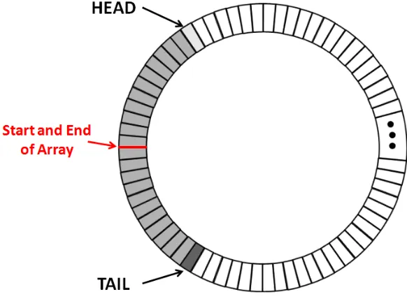
memory. The basic circular buffer shown in Figure 4.1 is composed of a couple of
pointers and an array of some data type. The two pointers reference the head and tail of
the data. The head points to the location in the array where the next incoming data is
placed. So, as data is received, it is placed at this location and the head is moved to the
next location in the array. The tail points to the location in the array containing the next
data that will be removed from the buffer. After the data is removed, the tail will be
moved to the next location in the array. When either the head or tail reach the end of the
array, they wrap around to the beginning of the memory array. Consequently, this wrap
around results in a buffer that is circular in nature shown in Figure 4.1. Since the buffer is
and write only involves one memory access, the increment of a pointer, and a few safety
checks. So, the processing overhead is relatively low.
Figure 4.1: Circular Buffer
While circular buffers are one of simplest techniques used in non-blocking coding
practices, it does have a few potential complications. First, there is the risk of a race
condition occurring. Consider an example where the buffer is empty so that the head and
tail point to the same location on the array. The head is incremented first and the process
is interrupted before the data is loaded. Thus, the pointers indicate that the buffer has data
when it is actually still empty. If the interrupting routine reads from the tail location, it
will get invalid data. This situation is easily prevented by having the head increment only
after the data has been placed in the buffer. Another type of race condition has the
potential to occur when the head or tail is accessed from more than one location. For
interrupted before the tail is incremented. If the interrupting routine attempts to read the
memory from the tail, this location will be read twice, and the next location will be
skipped. This problem cannot be fixed by reordering the memory access and pointer
progression. The only solution is to ensure that the head and tail each be accessed from a
single location.
Another complication is that, since the size of the buffer is constant, circular
buffers have the potential to overflow. One approach to solve this problem is to make the
buffer ridiculously big. This ensures that the buffer never has the chance of overflowing.
While this method may be necessary for critical applications, it would negate the point of
using a circular buffer (to make optimal use of memory). In either case, there is always a
chance that some condition will occur that fills the buffer. Therefore, it is important to
minimize the consequences of buffer overflow. The solution could be different
depending on the application. One application might require a flag to be set to stop
incoming data. Another application might be able to simply throw incoming data away
when the buffer is full. In either case, it is necessary to accurately determine when the
buffer is full. This would seem simple except for the fact that the head and tail will point
to the same location on the array when the buffer is full or empty. The key is to not let the
buffer completely fill up. However, due to fact that the buffer wraps around, it is difficult
to determine the amount left in the buffer using math. One of the simplest solutions is to
simply have a variable keep track of how much data is in the buffer. The variable needs
to be updated after the data has been place in the buffer for the same reasons as those
While the circular buffers are conceptually simple and efficient, there are a few
subtle problems that make them detail intensive to implement. However, circular buffers
are possibly one of the most effective techniques widely used in implementing
non-blocking code. Circular buffers can be made even more effective by eliminating some of
the details of implementation. This can be accomplished by making a generic circular
buffer that can be reused in multiple applications. This way, the detail intensive testing
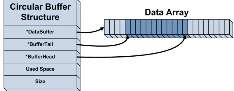
part of the implantation only has to be performed once. An example of this can be seen in
Figure 4.3. The circular buffer is composed of a structure that contains information about
the buffer and a memory array that stores the data. The structure stores a pointer to the
start of the data array. When the tail and head reach the end, it is important to know
where to start again. Pointers to the head and tail are also located in the structure. It does
not matter if the head and tail are literally pointers or just offsets from the start of the
array, as long as they accurately reference the locations of the head and tail. The circular
buffer for this research actually used offsets to simplify the math. The used space and size
variables indicate the amount of data in the buffer and the size of the buffer respectively.
By implementing a generic circular buffer, the main problem left is to prevent accessing
the head or tail from more than one spot. For most embedded applications, this is simple.
If the circular buffer is used for a hardware driver, then one end is accessed by the
hardware. This is commonly accomplished in an interrupt routine. The other end of the
circular buffer, in this case, is accessed by the application responsible for using the given
piece of hardware. Solving this problem can get more difficult when circular buffers are
flexible and have a wide variety of applications, as is the case for sensor networks. A
problem occurs when multiple applications need the data from one piece of hardware. In
these situations, it may be necessary to use a data manager.
Figure 4.3: Generic Circular Buffer
4.2.2 State Machine
The finite state machine is essential to non-blocking coding practices. Embedded
systems are generally used in applications that require microcontrollers to interface with a
considerable amount of hardware. Hardware interfaces usually operate at a different
speed to that of the main processor. Consequently, the processor is required to wait when
communicating with hardware interfaces. The waiting can be implemented with blocking
code or by using a state machine to keep track of the hardware’s progress. It is also not
uncommon for embedded systems to have more than one application that is constantly
running. In order for these applications to take turns using the processor, it is necessary to
keep track of the state of each process. Although it is possible under certain conditions to
would be highly unlikely to have an entire embedded system running off of non-blocking
code without the use of a state machine.
There are two types of state machines: synchronous and asynchronous. The
essential difference between these is that a synchronous state machine will only change
its state in sync with a particular event. In fact, another name for a synchronous state
machine is an event-driven state machine. In hardware, all the changes in a synchronous
state machine occur at a clock edge [8]. In other words, the clock functions as the event
that drives the state machine. The nature of software is such that the changes to the state
machine will occur in some type of function call. So the function calls work as the event
that drives software state machines. For the purpose of this thesis, state machines will be
referring to the event-driven type. Event-driven state machines can be further categorized
by the type of event that drives them. State machines used for hardware drivers are
usually interrupt driven. Most hardware interfaces have interrupts associated with them.
The interrupts trigger when certain aspects of the hardware interface, defined by the user,
change. These changes are usually designed to coincide with specific states in the driver’s
state machine. Therefore, it usually makes sense to have the state machine be driven by
the interrupt of the associated hardware. On the other hand, application level state
machines are typically driven by a scheduler.
Typically, in embedded systems, the state machines default to an idle state. Upon
receiving a start request from an application or hardware, the driver transitions to the
starting state of the desired action. On simple state machines, there may only be one
one shown in Figure 4.4. Each state is used for keeping track of the time or number of
events that have occurred. Unfortunately, an embedded system is rarely that simple.
Typically, the state machine will have multiple action sequences with their different
starting points. Each action sequence will usually have more factors determining the next
state other than the event driving the state machine. Sometimes, an error will occur in
hardware, and the hardware driver state machine needs to be able to account for the error
condition. It is evident that state machines can be considerably complex. The
considerable differences between each application prevent the easy reuse of a state
machine template. The complexity of state machines is probably one of the most
significant drawbacks to implementing non-blocking code.
Figure 4.4: State Machine
The complexity is not the only issue facing the use of state machines.
Synchronous state machines are critically dependent on the timing of the driving event. In
hardware driven state machine, the driving event is a clock edge, which is typically
an interrupt occurring. So, an important state transition will be missed if a condition for
transitioning the state machine occurs momentarily, and the driving event does not occur
during this time. For example, consider a situation where incoming data from a sensor for
an application is received into the applications buffer, but the applications task
responsible to process the data is not called before the data is overwritten. This will result
in the overwritten data never getting processed. It is not always necessary for driving
events to occur at a precise time interval, but it is necessary for them to occur often
enough to not miss any changes of conditions. The timing for applications and other task
driven state machines is usually handled by a scheduler. With a scheduler, it is important
for each task to follow the good citizen approach and release as soon as possible.
Otherwise, another task might miss a critical event.
Another problem is that each state machine requires permanent memory
allocation to keep track of the state and related variables. Good coding practices dictate
that one should avoid using global variables as much as possible for two reasons. First a
global variable permanently consumes a piece of memory which is a valuable resource.
Secondly, global variables decrease the readability of the code [9].
4.2.3 Callback Function
While callback functions are not essential to non-blocking coding practices, they
provide several beneficial services. Callback functions facilitate more efficient use of
memory and processing resources. One benefit to callback functions is that wasted
are reduced. Furthermore, memory used for flags that indicate when action is completed
is freed up as a result of the use of callback functions.
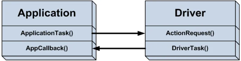
Callback functions are simply functions that are used to call the user back when a
particular action is complete. Consider a typical example represented in Figure 4.5. In
this case, an application task makes a function call to the hardware driver to perform an
action. What the application and action requested is not important. What is important is
that the action involves waiting for the hardware to respond. So, the hardware driver
starts the action in motion on the hardware, and then immediately returns control back to
the application task. The application then completes whatever else it needs to and returns
control to the scheduler. This is often simply involves the application saving its state. The
scheduler continues to provide the driver task its share of processing time to complete the
action. After the action is complete, the driver task will call the application callback
function to indicate that it is complete. The callback function can update the state
machine or a flag to let the application know that the action is complete. However, even
more importantly, if the application has any time-critical actions based on the ending of
the driver’s action, they can be in the callback function instead of waiting for the
applications task to be executed again.
The same thing can be accomplished with the use of global flags or a polling
function called from the application. With non-blocking code, there is already more than
enough permanent variables adding to the clutter and consuming memory. So,
eliminating the need for global flags can be a very useful accomplishment in
non-blocking code. Having a polling function inside an application task means that it will be
called every time. This might not seem like much of a cost in processing time, but, if the
application is not doing anything other than checking to see if the driver is finished, it is
doubling the processing cost of the application task at this time. Additional cluttering of
the software aside, this processing time can add up quickly. Since implementation
complexity is one of the largest limitations of non-blocking code, anything that can
simplify the code is a good thing.
4.3 Example Code
It is sometimes easier to see the difference of blocking and non-blocking coding
techniques by comparing an example of each style. The example code shown for both
cases is responsible for transmitting data using specialized hardware on the
microcontroller. The general method would be same for any of the common
communication protocols (UART, SPI, I2C, etc). These examples demonstrate how
blocking techniques are simpler to implement, and how the blocking techniques can be
optimized.
4.3.1 Blocking Code Example