Hardware and software development of the Anglescan tracking system

...

.41

Hardware and Software

Development of the

Anglescan Tracking System

the Anglescan Tracking System

By

Vito Dirita (BE Electronic Engineering)

Submitted in fulfilment of the requirements for the degree of

MASTER OF ENGINEERING SCIENCE

The University Of Tasmania

Department of Electrical and Electronic Engineering Hobart Tasmania. 1994

Supervisor: Mr. G. The' Submission Date: January 1995

DECLARATION:

I declare that this thesis is original except where due acknowledgement is given,'and the material has not been accepted for the award of any other degree or diploma.

I

N

DEX

Abstract p.1.1

Acknowledgements p.1.3

Thesis Outline p.1.4

General Notation and Terminology p.1.5

Chapter 1: Introduction:

Surveying Instrumentation

[1.1] Electronic Theodolites p.1.7

[1.2] Optical Tracking Systems p.1.12

The Anglescan Tracking System

[1.3] Anglescan: Principle of Operation p.1.16

[1.4] Sources of Errors p.1.21

[1.5] Chapter Summary p.1.25

Chapter 2: Hardware/Software Design:

The Anglescan Optical System

[2.0] General Overview p.2.2

[2.1] Optical Transmission System p.2.4

[2.2] Photo-Detector Optics p.2.6

The Anglescan Electronic System

[2.3] Block Diagram of Electronic System p.2.7

[2.4] Target Measurement Card p.2.11

[2.5] Azimuth and Elevation Interface Card p.2.17

[2.6] Analog Signal Processor Card p.2.27

[2.7] Microprocessor Card p.2.33

[2.8] Front Panel Display Card p.2.36

The Anglescan Software System

[2.9] Anglescan Software Description p.2.39

[2.10] The User Menu Interface p.2.42

[2.11] Chapter Summary p.2.45

Chapter 3: System Identification:

Introduction to Identification

[3.1] Introduction p.3.2

[3.2] Identification Techniques p.3.2

[3.3] The Servo-System Model p.3.9

[3.6] Recursive Least Squares p.3.17

[3.7] Extended Recursive Least Squares p.3.21

[3.8] Least Squares with Offset p.3.24

[3.9] Higher Order Models p.3.27

[3.10] Reduced Coefficients Model p.3.28

[3.11] The Constant Trace and Forgetting Factor p.3.29

[3.12] Identification of Stiction and Coulomb friction p.3.32

Measurements and Model Validation

[3.13] Summary of Azimuth and Elevation Models p.3.35

[3.14] The System Identification Program p.3.36

[3.15] Chapter Summary. p.3.40

Chapter 4: Controller Design:

Introduction

[4.1] Chapter Outline p.4.2

[4.2] Experimental Set Up p.4.3

[4.3] The Anglescan Measurement Model p.4.5

Compensator Design

[4.4] The Proportional Controller p.4.18

[4.5] The Pole Placement Controller p.4.26

[4.6] Chapter Summary p.4.36

Chapter 5: Instrument Calibration:

Mathematical Background

[5.1] Introduction p.5.2

[5.2] Derivation of Calibration Equations p.5.6

[5.3] Linearization and Solution by Least Squares p.5.9

Simulation/ Results

[5.4] Computer Simulation p.5.17

[5.5] Current Calibration Implementation p.5.23

[5.6] Chapter Summary p.5.26

Chapter 6: Discussion/Conclusion:

[6.1] General Applications p.6.2

[6.2] Future Development Work p.6.4

[6.3] Summary of Contributions p.6.7

Chapter 7: Appendix:

Mathematical Symbols Table

[7.1A] General notation p.7.2

[7.1B] Mathematical Symbols p.7.3 [7.1C] Keywords and Definitions p.7.5

References

[7.2A] Futher Reading p.7.6

Mathematical Derivations

[7.3A] Least Squares Estimation p.7.13

Simulation Programs:

[7.4A] System Calibration Simulation program (SYSTCAL2C) p.7.14 [7.4B] System Identification program(SYSTIDE.C) p.7.14 [7.4C] Proportional Control System Simulation program(SYSTPROP.C) p.7.14 [7.4D] LQR Control System Simulation program(SYSTLQR.C) p.7.14 [7.4E] PPDControl System Simulation program(SYSTPPD.C) p.7.14

Circuit Diagrams

[7.5A] Signal Processor p.7.16

[7.5B] Target Measurement Card p.7.17 [7.5C] Motor Driver Card PWM p.7.18 [7.5D] Front Panel Display Card p.7.19 [7.5E] Motor Driver Card HID Controler p.7.20 [7.5F] System Wiring Diagram p.7.21 [7.5G] Joystick Manual Interface p.7.22

Aglescan Tracking Software

[7.7A] The User Interface p.7.23

[7.7B] PIO Address Map p.7.26

Photographs

Abstract:

In this thesis, the author describes all the developmental work of an automated surveying

tracking theodolite referred to as The Anglescan Tracking System. This system consists of an optical system, an electronic system (with detailed schematics and printed circuit

artwork, included) the software system which is approximately 100 pages of C source

code, system identification and controller simulation, modelling and design, and finally

instrument calibration and testing effort over a 2 year period.

The project is a collaboration between the Department of Electrical and Electronic

Engineering and the School of Surveying at the University of Tasmania. It is supported

by an ARC university research fund granted to the School of Surveying over a two year

period.

The initial investigation into the feasibility of the project was carried out by Dr. A. Sprent,

then at the North East London Polytechnic (Sprent, 1.12). During this time the optical

system of the instrument was developed. Following this investigation, it was decided to

further undertake the continuation of the project as a Master's Degree in order to develop

the electronics, measurement, tracking and control software.

The Anglescan system is similar to a standard surveying theodolite mounted on a tripod

and capable of determining the position of a retro-reflective mirror based within the

instrument's field of view with respect with its optical centre of field (in both azimuth and

elevation planes). This involves a new and different technique for target location than the

currently existing electronic theodolites (see sections 1.5, 1.6).

One of the main advantages of this method is the improved target locating accuracy, it has

been field tested with an accuracy of +1-1 second of arc, and simplicity in optical design.

The disadvantages however include increased complexity of both the hardware

(electronics), software, and calibration involved.

The instrument deviates from a standard theodolite in that it has been fitted with precision

DC servomotor drives on the azimuth and elevation axes for target tracking. The

servomotors also include optical rotary encoders for measurement..

While tracking, the system operates by continuously locating the target mirror with

respect to its centre of field of view, then applying a feedback control signal to the

azimuth and elevation motors in order to re-centre the instrument directly onto the target,

Chapter 1: Introduction P.1.2

Part of the objectives of this work is to design the necessary hardware and software to

achieve this task, this includes the design of a return (laser) analog signal processor card,

the design of a target position measurement card, and azimuth/elevation servo motors

interface cards (azimuth card and elevation card).

Furthermore, the project also requires the design of an appropriate target acquisition and

control loop strategy to allow smooth and accurate tracking of a moving target. A number

of control system designs have been investigated, including proportional control, pole

placement design and linear quadratic control. We have also used system identification

techniques to obtain an accurate model of the plant which is necessary for controller design and simulation.

To achieve the high precision required in measurement, it is necessary to calibrate the

instrument. The calibration method is a complex procedure which uses least squares

techniques to produce the required calibration accuracy (this is discussed in detail in

section 5).

The instrument finds applications in areas such as monitoring earth movements, motion of

large structures such as building and bridges, locating earth working machinery such as

tractors, bulldozers, graders, concrete and asphalt paving machines where an accurate

level surface is required.

Another application of particular interest is in surface contour mapping where we require

to map a 3 dimensional surface (obtain the surface contour or topography), this

application is a slightly more complex problem requiring the use of two instruments, this

then becomes a multivariable control problem.

As a result of this research work, one paper was presented at the IREECON-91 conference in Sydney and is published in the proceedings [Dirita 1.13]. Another paper

was presented at the CONTROL-92 conference held in Perth in November 1992 and is published in the proceedings [Dirita 4.4].

Acknowledgements:

The author is grateful to many of the members of academic staff both in the School of

Surveying and Department of Electrical and Electronic Engineering, whose assistance has

contributed greatly to the preparation of this thesis.

In particular, my supervisor Mr. G. The' for his constant guidance and encouragement

during the course of the project.

I would also like to thank my second supervisor Dr. A. Sprent for providing both the

research project and financial assistance throught the ARC grant.

Finally, my thanks to Mr. K. Bolton in the Physics department, for the preparation of

printed circuit artwork photonegatives from the Protel AUTOTRAX gerber files, and

etching the printed circuit boards.

V. Dirita

The University of Tasmania

Chapter 1: Introduction P.1.4

Thesis Outline:

The thesis covers a broad aspect of engineering disciplines such as embedded software

design, hardware design, control system design and simulation, system identification,

instrument calibration, and testing. Each has been arranged into individual chapters as

outlined below:

Chapter 1: Introduction Starts with and introduction to the electronic theodolite and

surveying instrumentation, it also describes the principles of some existing automatic

optical tracking systems. Then an introduction to the principle of operation of the

anglescan system is given.

Chapter 2: Hardware and Software Design Covers a detailed overview of the

principle of operation, and an introduction to the optical system, including the

measurement technique and potential sources of errors. This chapter is grouped into 3

parts: The first is a description of the optical system, the second section is a detailed

description of the entire electronic system which is based on a dedicated bus backplane

and low end Z80 microprocessor (due to be upgraded to a full 32 bit off-the-shelf

processor system). The third section of this chapter is a functional decomposition and

top-down design of the Anglescan tracking software system totally developed in C high

level language, it also describes the user menu interface and command structure for

operating the instrument.

Chapter 3: System Identification This chapter is devoted to system identification.

It describes the most common techniques of identification, we also develop the structure

of the servosystem model, then proceed to apply least squares techniques for estimating

model coefficients using a pseudo random binary excitation source. Several models are

compared both higher order and reduced order form. The model are then verified by step

response simulation and compared with the real system response.

Chapter 4: Controller Design Covers the subject of controller design. We

commence with the transient behaviour and steady state performance of the

uncompensated system. Various forms of controller compensation are subsequently

applied, these include the most common implementations of Proportional control and

Pole placement design. These models are verified by computer simulation and compared

with the response from the real system. We also describe the measurement model which

is included in the control system model.

Chapter 5: Instrument Calibration Covers the topic on instrument calibration. Instrument calibration requires the derivation of a system of equations describing the

measurement data as a function of calibration unknowns (which turn out to be non linear),

applying linearization techniques and least squares for parameter estimation. This is

verified by computer simulation.

Chapter 6: Discussion and Conclusion This chapter covers typical applications of the anglescan system, including surface topography determination, tracking of moving

targets and general survey use. We also discuss possible areas for future development. A

discussion and conclusion is also included.

Chapters 7: Appendix Contains a table of mathematical symbols, general notations used, references for further reading, a listing of the simulation programs used, schematic

diagrams for each board, some photographs of the system, and information on the user

menu interface. The anglescan software system is too long and will not be reproduced in

the thesis.

General Notation and Terminology:

Scalars: Scalars are denoted in lower case plain text, ex: x

Vectors: Vectors are denoted in lower case plain underlined text, ex: 0

Matrices: Matrices are denoted in upper case bold text, eg: H

Subscripts: - Iteration number, eg: 0k= kith iteration

- Variables belonging to same subset, eg: {al, a2,a3,a4 }

- Sampling: eg: xk=kith sampled value of x(t) at t.k.T

Constants:

Estimates:

Transformed values:

Time derivatives:

Shift Operator:

Denoted in upper case plain text, ex: K

A Is the original variable annotated by a hat symbol: eg: 3(

Are represented in upper case thus H(s) and H(z) are the laplace transform and the Z transform.of h(t) respectively.

Represented in dot notation: eg 6 = de/dt

Chapter 1: Introduction P.1.6

Chapter 1

Introduction

[1.1] Electronic Theodolites:

Here we discuss the various components and functions of a basic electronic theodolite

prior to describing the Anglescan Tracking System. Refer to Kennie [1.6], Deumlich

[1.8], and Laurilla [1.9] for further references on theodolite contruction. Theodolites

traditionally have been made for two different applications:

[a] Low accuracy instruments which are gnerally simpler, used for simple technical

measurements such as on construction sites. Accuracy of the order of 1/10 arc

minute is generally sufficient.

[b] Instruments of medium to high precision are used for triangulation, traversing and

levelling , and for engineering surveys. Precision instruments are required for

astro-geodetic measurements like azimuth, latitude, for triangulation and first or

second order levelling.

A theodolite is generally required to perform the following functions:

(a) Levelling and alignment.

(b) Angular azimuth and elevation measurements. (c) Distance measurement (DME).

Theodolite Construction:

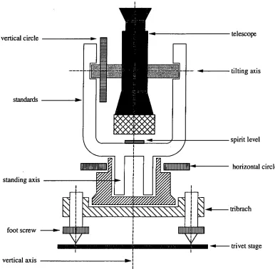
The theodolite consists of the following main parts: referring to Fig.1.1, a fixed base with

tribrach, a movable upper part and telescope. The base, with the tribrach, is attached to

the tripod head and is levelled by adjusting three foot screws. On the upper part (the

alidade), which is rotatable about the vertical axis and also contains the horizontal reading

circle and a spirit level (circular or cylindrical). The two standards for the tilting

(horizontal) axis are fixed, bearing the telescope with the sighting axis and vertical circle.

The vertical circle reads zero when the telescope is pointing to the vertical (zenith) and 90

degrees when sighting the horizon. The horizontal circle is resettable in any direction.

For approximate levelling of the base, a circular (bull's eye) spirit level is used to provide levelling in 2 planes directly; for more accurate levelling however, a tubular level is used

which provides levelling in one plane only, thus to level in both planes with the tubular

foot screw

vertical axis vertical circle

standards

standing axis

111111111111111111

111111111'111111111 iffi11111111 liii 111111111111111111

Chapter 1: Introduction P.1.8

The instrument is centred over the station point by means of a plumb-bob or a built in

optical plummet, and trivet stage (or stage plate) carrying the theodolite. The trivet stage

can be moved laterally on the tripod head until the plumb-bob lies over the ground mark.

Fig 1.1 below illustrates the components of a basic theodolite.

telescope

tilting axis

spirit level

horizontal circle

tribrach

trivet stage

Fig. 1.1 Basic theodolite construction

(a) Levelling and Alignment

Traditionally, consisting of spirit levels or tubular levels. Currently however, electronic

levels utilize inverted pendulum techniques, and laser collimation techniques to achieve

higher accuracy are being used, fig.1.2a below shows the construction of a standard

Tubular spirit level, consisting of a cylindrical glass tube filled with a low viscosity liquid

such as alcohol or ether.

Fig 1.2b below also shows the construction of a circular (Bull's eye) level, allows

alignment in both planes, sensitivity is generally not better than 8 seconds of arc, used for

quick-approximate levelling of a plane.

Chapter 1: Introduction P.1.9

bubble

housing

ether

glass tube

bubble

housing

ether

glass cylinder N

ei

Fig. 1.2a Fig.1 2b

Fig. 1.2 Tubular and bull's eye spirit levels.

Sensitivity for high precision levels is about several seconds of arc. Levels for surveying

instruments generally have nominal sensitivities of 10, 15, 20, 60, 120 arc sec.

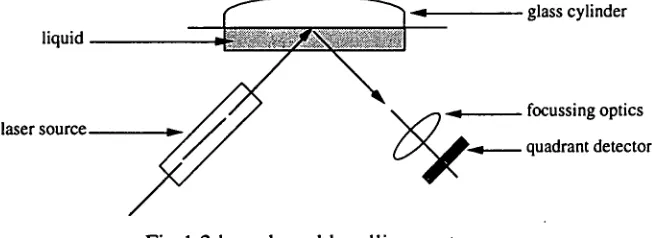
Electronic levels currently use a laser/liquid levelling system. The liquid is illuminated

with a laser source, the reflected beam is focussed on to a four quadrant detector, thus the

ratiometric output of the quadrant detector is directly proportional to the angle of

inclination. The quadrant detector is described further in section 1.2.

Accuracy with this method is better than 0.2 seconds of arc, and generally used in first

order geodetic levelling. Fig 1.3 below illustrates this technique:

glass cylinder

focussing optics

quadrant detector liquid

laser source

Fig. 1.3 laser based levelling system

(b) Angular Measurements:

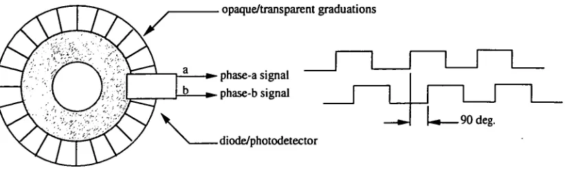
Modern electronic theodolites incorporate an electronic circle reading system. This

consists of a photolithographically coded circle on a glass plate on which a series of

opaque/transparent sections have been etched, with photoelectric detector and photodiode.

Two square wave outputs are provided phased 90 degrees apart which determine the

opaque/transparent graduations

phase-a signal phase-b signal

I

rotating glass circle

a signal

diode/photodetector

displacement: 0 = n.(1) + 64)

Fig. 1.5 Electronic circle scanning measuring system

b-signal

diode/photodetector

Chapter 1: Introduction P.1.10

Fig. 1.4 Electronic circle measuring system

More advanced theodolites use a moire' fringe pattern, this gives coarse and fine

measurements, similar to Fig. 1.4 above with sinuousoid rather than rectangular wave

outputs.

The coarse component is obtained by squaring the sinuoid outputs from the encoder and

feeding directly into a digital counter, this gives resolution to about 30 seconds of arc.

The fine measurement is obtained by interpolation ie: measuring the phase angle of the

moire' signal to improve the resolution to 1% of the moire' period ie: about 0.3 seconds

of arc.

Yet another method currently used is based on a dynamic circle scanning technique. The

circle is divided into N opaque/transparent segments. A drive motor rotates the glass

circle past two photodiode/photodetectors, one set is fixed (A), the other (B) rotates on a

separate plate where the theodolite is mounted. Refer to Fig. 1.5.

The angle can be computed from measurements of fine and coarse data from the phase

difference of the two signals. This is one of the most commonly used methods for the

more accurate measuring theodolites.

The displacement (8) is the integer count n multiplied by the line separation plus the phase

difference between the two detectors providing the coarse measurement. Accuracy is about 0.5 arc seconds.

The method we have adopted for azimuth/elevation measurements is yet different from the

others described above, (refer to section 2.5 on the method we used for fine positioning

measurement).

(c) Distance Measurement:

Traditionally, distance measurement (DME) has been based on time-of-flight microwave

radar techniques (tellurometers). Current methods are generally electro-optic based on

either:

(a) phase difference techniques. (b) time of flight (or pulse echo).

Microwave based distance measurement equipment (DME) requires an active transponder

to provide a return signal. Advantages of microwave include increased range and

operation over all weather conditions.

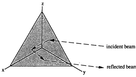
Laser based (LIDAR) DME equipment requires the use of a retro-reflector prism (corner

cube reflector) or acrylic retro-reflector which return the incident beam along the same

path. The main disadvantages of laser based DME systems is the dependence upon good

atmospheric visibility and optical alignment with the reflector.

Phase Difference Method: This method uses an intensity modulated laser source.

The return signal is phase compared to the transmitted signal, the distance is an integer

number of wavelenghts n plus a fraction of wavelenght obtained from phase comparison:

2D=n.+AX. 1 1

By taking a set of measurements, and switching wavelenghts, then both ni and A may be

estimated. Modern instruments selectively scan through different modulation frequencies and then solve for A and ni by least squares. Range is generally up to 51(m, accuracy is

of the order of +1-5mm.

— incident beam

— reflected beam

Chapter 1: Introduction P.1.12

Pulse Method: The return echo of a short high energy pulse is used in time-of-flight measurement, the distance is given by the equation:

2D = C.At (1.2)

where C=speed of light, dependent upon atmospheric conditions. This technique works

well over long distances. Fig. 1.6 below shows a typical corner cube reflector required by

most electro-optic DME equipment:

Fig. 1.6 corner cube reflector

[1.2] Optical Tracking Systems:

Optical laser tracking systems measure the position of a retro-reflective target placed

within the instrument's field of view with respect to its optical centre of field. This

information is then fed back into a control system driving azimuth and elevation

servo-motors, hence enabling the tracking system to re-centre itself on the target. One

advantage of laser tracking systems is that they can be designed to be small, portable,

compact and relatively lightweight.

Ample literature exists on this subject (see references 1.1, 1.3, 1.5 and 1.7 in the

appendix 7.2A). One example is the star tracker on spacecraft systems, star trackers are

passive instruments (rather than using active laser systems) in that they only detect the

position of a point light source such as a bright stellar object. Tracking systems usually

operate in two basic modes:

(a) target search mode.

(b) tracking mode.

In search mode, the instrument scans a prescribed space sector looking for a target, if the

target is detected, then it is continuously tracked.

telescope mirror

retro-reflector

centre of field

laser transmitter

detector

mirror

Normally angle tracking is required, although sometimes range tracking is also needed.

Angle tracking implies continuous estimation of the target angle coordinates, this is

typically achieved by the means of a mosaic sensor (eg: CCD or four-quadrant detector)

which is described below.

(a) Target Position Estimation:

The optical tracker senses the target position with respect to its optical centre of field by

focussing the target's image onto a sensor located on the focal plane. The two most

common detectors are: the CCD array and the four quadrant detector.

Fig. 1.7 below illustrates the basic principle. A laser beam is transmitted along the optical

centre of the instrument, the return signal is focussed by a parabolic mirror onto a detector

(either type), depending on the position of the retro-reflector will directly determine where

on the detector the return laser signal is focussed.

Fig. 1.7 optical layout of typical tracking system

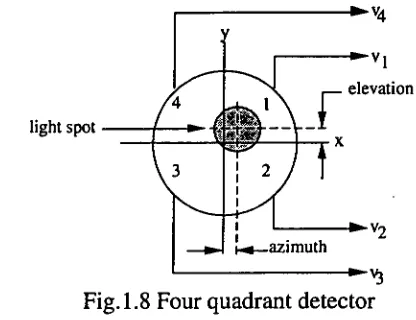
Four Quadrant Detector:

This being the simplest, the detector is of the type shown in Fig.! .8 below. It consists of

four separate photo-sensitive detectors placed on a circular substrate. The ratiometric

values between outputs of the four sensors determines the position of the retro reflector in

azimuth and elevation planes. Accuracy with this system is about 20 seconds of arc.

Equations 1.3A and 1.3B below give the relationship between position of the target as a

elevation

light spot

v3 Fig. 1.8 Four quadrant detector

Chapter 1: Introduction P.1.14

Azimuth and elevation are given by: (where v1,v2,v3,v4 are the individual output

voltages of each quadrant)

(V

1 + v2 ) (v3 + v4 )

AZIMUTH oc ₄

E

'

(1.3A)

ELEVATION oc (vi ₊

v4) (v2 + v3 ) 4

E

(1.3B)

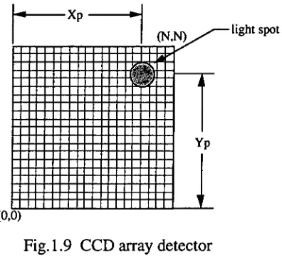
CCD array:

Another common technique is to use a CCD array on the focal plane. The intensity

distribution formed is usually a gaussian function over the two dimensional image plane,

figure 1.9 below illustrates the technique. Equations 1.4A and 1.4B give the relationship

between individual element output and azimuth/elevation.

N N

E E

j=i xp - N N

i.1 J.1

N N

E E

Yp N N

E

(1.4A)

(1.4B)

Typical CCD detector array is shown in Fig. 1.9, where xp and yp are the centroid of the light spot with respect to the lower left hand (datum) point (0,0), vij are the individual

output voltages from each element of the array with the lower left hand corner (0,0) element voltage being voo and N is the number of elements ie: NxN array.

Chapter 1: Introduction P.1.15

This method is generally more accurate than the four quadrant photodetector system:

h-XP

111•111•••••11111111111111111111111

•••••••••

Yp

(0,0)

Fig. 1.9 CCD array detector

Atmospheric disturbance such as scintillation caused by refractive index gradients,

atmospheric scatter, vibrations in the optics, and measurement errors all contribute to

apparent target jitter. For a moving target, velocity can be estimated in the presence of

jitter by correlation or Kalman filter techniques.

Once the target position is estimated, the tracking system computer applies a correction

signal to the servo motors. The correction signal rotates the instrument such that the

centre of field of view is directly on to the target. Displacement is then measured by the

main optical rotary encoders on the servo motors. This technique provides accuracy to

only +/-1 step count on the rotary encoder.

An alternative method would be to rotate the servo motors by an exact integer number of

steps and then measuring the position of the target with respect to the instrument's centre

of field. The accuracy of this technique would then be dependent on the optical

measurement system rather than the servo-motor encoders. The target's position is then

given by:

x = n.(1) + x (1.5A)

y = n.(I) + yp (1.5B)

where x and y are the overall displacement, n=number of integer steps, 4)=step size, and

(xp,yp) is the centre of the target given by Eqn.1.4A and 1.4B. This is the method which

Y 1 1

horizontal beam

elevation

1411P` azimuth

measurement zenith

Y

1

Chapter 1: Introduction P.1.16

[1.3] Anglescan: Principle of Operation:

The anglescan system is different from any of the conventional techniques described in

the previous section. Fig.1.10 below illustrates the overall simplified system including

the co-ordinates used:

Fig.1.10 overall anglescan system

Referring to Fig.1.10, the instrument operates by projecting a cross, the two orthogonal

lines forming the cross are labelled: vertical beam and horizontal beam. The instrument

then rotates this cross in a circular path with a radius of 0.5 degrees, note that the vertical

beam remains vertical always, and the horizontal beam remains horizontal always.

To detect and locate a target, it must be placed within the field of view of the instrument

which is defined by the extent of the circle. Both the horizontal and vertical axes span at

twice the diameter of the circle, that is 2 degrees. The cross rotates at 30 times per

second.

Target position is measured each time the cross completes one full rotation, that is at a rate

of 30 times per second. The target position data is subsequently used to generate a

control error signal to the servo-motors such as to re-orient the instrument's centre of field

directly on to the target. A detailed overview of the hardware is presented in chapter 2.

The instrument has a maximum range of about 800 meters, the range is determined by the

size of the reflecting target.

(a) Target Position Estimation:

The target position is measured by projecting a set of othogonal laser beams (diagram

1.11A, 1.11B, 1.11C, 1.11D below). The laser beams form a cross, the horizontal

beam is labelled Hbeam, and the vertical beam is labelled: Vbeam, also refer to fig. 1.10

above. The cross is then made to rotate along a circular path of radius equal to the field of

view of the instrument. The laser source used is a 3mW HeNe visible (red) laser.

Referring to Fig.1.11A to 1.11D, two orthogonally projected beams forming a cross

rotate along a circular path clockwise. Assume that an index pulse is generated by the

rotary encoder (refer to fig.2.1) each time the centre of the cross passes through the top

dead centre of the circle. The index pulse acts as a zero reference for the angular measurements of a 1,a2,a3,04.

Fig.1.11A: Initially the vertical beam (designated: Vbeam) intersects the target mirror

from the left hand side, a return pulse is detected, the first measurement of al is obtained from the optical rotary encoder.

Fig.!.! 1B: Next, the Horizontal beam (designated: Hbeam) intersects the target from above, producing an angular measurement of a2 from the rotary optical

encoder.

Fig.1.11C: Again, the vertical beam again intersects the target from the right hand side producing an angular measurement of a3.

Fig.1.11D: Finally, the horizontal beam again intersects the target from below producing the last angular measurement of a4.

The cross rotates 30 times per second, this value can be adjusted by varying the voltage

on the motor. The sampling rate and position determination is set to 33 msec, also the

loop time for closed loop control system analysis is 33 msec.

Measurements of ai and a3 determine the target azimuth:

1 = R. sin (a1) (1.6A)

X

3 = R. sin (a3) (1.6B)

AZIMUTH = —₂ (X_I + X

Chapter 1: Introduction P.1.18

Measurements of a2 and a4 determine the target elevation:

Y₂ = R. cos (a2) (1.7A)

Y₄ = R. cos (a4) (1.7B)

1

ELEVATION = —₂ (Y₂ + Y₄) (1.7C)

equations 1.6C and 1.7C give geometric centre of target. Thus positioning accuracy is

determined irrespective of the size of the target.

The method described above provides positioning accuracy to about +/-1 arc second. It

has some inherent problems however, which are discussed in section 1.4.

H beam

azimuth

Fig.1.11A First intersection of target

V beam

Top dead centre

y

Pix2Y2)

+

azimuth

r

H beam

: elevation

x

Hbeam Chapter 1: Introduction P.1.20

Fig.1.11C Third intersection of target

Top dead centre

Vbeam

H beam

P(XY) _{4 4 4}

\

elevation X R

.16-1.- azimuth

Fig.1.1 1D Fouth intersection of target

[1.4] Sources of Errors:

One of the advantages of this technique is the accuracy and simplicity in optical design, it

has a number of pitfalls however including target positioning ambiguity, beam

orthogonality, location of index pulse, and relative motion of target with respect to the

tracker. Most of these problems can be resolved with calibration (refer to chapter 5) or

from simple geometric tests in the anglescan software.

(a) Target Positioning Ambiguity:

Target positioning ambiguity can result when the target is placed in either quadrant 3 or 4

of the circle, Refer to Fig. 1.12 below:

Vbeam

H beam

Fig.1.12 target ambiguity condition

When the target is located in either one of quadrant 3 or 4, then the first time the beam

intersects the target is when the horizontal beam passes through from above giving the first measurement of oci. The data sequence is then HVHV as opposed to the previous

description (see Fig. 1.11A) where the vertical beam strikes first producing the data

sequence of VHVH.

When the condition demonstrated by Fig. 1.12 occurs, the computation of azimuth and

H beam

h

horizontal beam error

(1) v vertical beam error

Chapter 1: Introduction P.1.22

x = [ sin (a2) + sin (ad ] (1.8A)

y = [ cos (a 1) + cos (a3) ] (1.8B)

Despite this problem, position ambiguity can be easily resolved by a simple geometric

test conducted by the software.

(b) Beam Orthogonality:

The projected horizontal and vertical beams cannot be guaranteed to be truly othogonal.

Additionally the horizontal beam cannot be assumed to be truly horizontal (ie: parallel to

the horizon), and the vertical beam cannot be assumed to be truly vertical.

Fig. 1.13 below illustrates the problem, the errors are caused by optical and mechanical alignment. Generally the values of Ov and Oti are to within +1-5 degrees. To maintain

constistent instrument accuracy, we shall determine the horizontal and vertical beam error

during the calibration stage (discussed further in chapter-5).

Vbeam

Fig. 1.13 Horizontal and vertical beam errors

For applications requiring alignment or levelling, this error condition should be resolved

accurately.

V beam

index Ip

target

(c) Index Pulse:

So far, the assumption has been that the reference (zero index pulse) occurs at the exact

top dead centre of the circle. This is however not the case as the index pulse can occur

anywhere within the 360 degrees depending on the mechanical assembly of the optical

rotary encoder. Although the position of the index pulse remains constant (mechanically

fixed) it is an unDvn parameter which needs to be determined from instrument

calibration. As the index pulse is non zero, equations (1.8A) and (1.8B) are subsequently modified to accommodate for this condition. Referring to(_79:6 ations 1.9A and B below,

we define Ip as the angular position of the index pulse with respect to the top dead centre:

x = [ sin (a2 - I p ) + sin (a4- I p )] (1.9A)

y = —2-- [ cos (a 1 - I p ) + cos (a3- I p )] (1.9B)

Fig. 1.14 illustrates the condition where the index pulse occours in the fogi quadrant.

Fig.1.14 index pulse offset

H beam

(d) Relative Motion of Target:

The relative motion of the target with respect to the instrument introduces positioning calculation errors at the end of the sampling instance. The end of the sampling occurs on

Chapter 1: Introduction P.1.24

Refering to Fig. 1.15 below, and considering only motion effects on the azimuth position

calculation: when the target is at

a

By the time the beam intersects the target at P3, the target would have moved to point b.

Finally, when the beam reaches the top dead centre to complete the sampling cycle, all

four measurement are available, the target may have moved to point

c.

As the calculation of azimuth is a geometric average between measurements obtained at

P1 and P3, the tracking computer will thus estimate the target azimuth to be the midway between P1 and P3 ie: target AZJNIUTH=(x +x3)/2. This error is by far the most important

while tracking a moving target and can introduce instability in the closed loop control

system.

Vbeam

top

PI

H beam

target motion

X \ 1

,..._____ ,x,1 x 3

P3

N

N

Fig. 1.15 apparent target motion within fov

In section 4.3 we introduce the effects of apparent target motion into the control system

model and show that the system's overall margin of stability is actually reduced due to

this measurement process. Intuitively however, we can see that the control loop can

overcompensate when the target is actually closer to the centre than the calculation

indicates, or undercompensate when the target is actually further from the centre than the

calculations indicate.

[1.5] Chapter Summary:

In this chapter we presented some of the basic concepts behind the construction of an

electronic theodolite including the three main uses of a theodolite: (1) Levelling, (2)

Angular measurement, and (3) Distance measurement. We have shown the method by

which the theodolite is able to achieve each of these objectives.

We also discussed the basic construction of an optical tracking system, and the means of

determining the angular position of a target placed within the field of view of the

instrument.

We have finally introduced the anglescan system and the principle behind the

measurement technique. The anglescan system essentially comprises of a combination of

the two instruments described above but with a totally different technique for the

determination of the target position.

Such instruments currently do exist as commercially available theodolites with target

tracking capabilities, however the anglescan system is the only one with this kind of

measurement technique and subsequently most of the work on the instrument would be new and innovative.

In the following chapters we will discuss the different aspects of the anglescan system and

Chapter 2: Hardware and Software Design P.2.1

Chapter-2

Hardware and Software Design:

[2.0] General Overview:

Fig.2.0 below shows a detailed assembly of the main components of the anglescan

tracking system. The system consists of two parts: (a) the Anglescan optical and

mechanical system, generally mounted on a tripod and (b) the Anglescan electronic and

software system. The electronic system consists of 6 boards interconnected via a

dedicated backplane bus, and power supply. There is also a front panel LCD display and

keyboard.

target reflector

photodetector , filter __-_-_-:--- field stop::.--

dove prism

laser source beam expander

beam splitter pentaprism dc motor

rotary encoder

rotating wedge prism

worm drive

fresnel lens

reflector

pivoting axis

worm drive

elevation motor

azimuth motor

front panel display card microprocessor card azimuth interface card

elevation interface card analog signal processor card target measurement card #1 target measurement card #2

alluminium base power supply

Chapter 2: Hardware and Software Design P.2.3

(a) Optical System

Referring to fig.2.0, a 3 mW HeNe laser source is used, the output of the laser is

reflected by a dove prism into a beam expander. The laser beam is thus expanded from a

single point into a line. The output of the beam expander is fed into a beam splitter a

pentaprism and a rotating wedge prism. This has the overall effect of projecting a rotating

cross (refer to fig.2.1).

When the laser cross strikes a target retro-reflector, a return pulse is produced. The return

pulse is reflected into a fresnel focussing lens, a field stop and interference filter, and

photodetector placed on the focal plane. The output from the photodetector is fed into the

analog signal processing card.

Servomotors are mounted on the azimuth and elevation axis. Each servomotor consists of

a 24V DC motor and worm drive assembly, it also includes an optical rotary encoder for

positioning measurements.

(b) Electronics System:

There is a separate power supply for the HeNe laser which generates about 7KV nominal

output voltage mounted near the laser. The laser output power is typically 3mW. The

existing laser will eventually be replaced by a semiconductor infrared laser which operates

at much lower voltages (3Vdc). Figure 2.2b illustrates the second part of the anglescan

system which is the electronic system and interface to the optical and servo-system. The

electronic system consists of the following cards:

(1) Front panel keypad and LCD display card.

(2) Z80 microprocessor card with 32K RAM, 32K EPROM, and dual UART.

(3) Azimuth servomotor interface card with azimuth encoder positioning measurement. (4) Elevation servomotor interface card with elevation encoder positioning measurement. (5) Analog signal processor card for detecting and processing return pulses.

(6) Return pulse measurement card #1. (7) Return pulse measurement card #2.

(c) Power Supply:

The power supply consists of two separate mains step down transformers with one

supplying +12V to the high voltage inverter used by the HeNe laser. The second

transformer supplies +/-18V unregulated to all the individual cards via the backplane bus,

each board has its separate voltage regulators typically +5V and +/-12V for CMOS and

analog supplies.

dove prism

HeNe laser

mirror

projected cross

beam splitter

pentaprism

shaft encoder

Counter Index

dc motor

rotating wedge prism

[2.1] Optical Transmission System:

The optical transmission system is shown in Fig.2.1. It consists of a 3mW HeNe visible

red laser and a dove prism reflecting the beam into a beam expander. The purpose of the

dove prism is to allow the laser and beam expander to be mounted side by side thus

reducing the overall physical size of the instrument.

The point beam passes through a collimator and beam expander thus producing a fanned

beam with a divergence of 2.0 degrees along one plane, the output of which is then

separated into two equal intensity beams via a beam splitter. The first half forms the

vertical component of the projected cross, whereas the second half is rotated by 90

degrees with a pentaprism and is then projected to form the horizontal component of the

cross.

The rotating wedge prism is a circular disk made of optical glass attached concentrically to

a dc motor. When the wedge prism is rotating, the projected cross rotates along a circular

path, the radius of which is a function of the refractive index and geometry of the wedge

prism. Currently the prism causes a deflection angle R of 0.5 degrees radius.

Fig.2.1 Anglescan optical system

The motor and gearbox combination rotates the wedge prism at a fixed rate of 30 Hz. The

Chapter 2: Hardware and Software Design P.2.5

The shaft encoder measures the position of the cross along the circle with a resolution of

10,000 counts per revolution, it also generates a reference index pulse once per

revolution. This index pulse is used as a sampling reference to reset and then restart the four counters which measure the values of a 1 ,a2,a3,a4 . Refer to section 2.4. and

fig .1.11A,B ,C,D.

signal processor

hybrid photodetector

field stop

interference filter

hood

fresnel lens

return signal

projected cross

index

L

dc motor/gearbox

rotary optical encoder

[2.2] Photo-Detector Optics:

The detector optics consists of a large mirror (reflector), a Fresnell focussing lens, a field

stop and a narrowband interference filter with the passband centre at the laser wavelenght.

This effectively removes a high proportion of ambient background light. The raw signal

is detected by a hybrid photodetector-amplifier which provides low noise and low output

impedance.

Fig.2.2 Photodetector optics

This signal is then fed to an analog signal processor board (described in section 2.6).

Fig. 2.2 illustrates the design of the detector optics.

The photodetector signal is nominally 5 mV peak to peak amplitude at a maximum range

of about 800 metres. The noise level has approximately the same peak amplitude. This is

the limiting factor in determining the maximum range and signal detection at this range is

front panel display card

microprocessor card azimuth interface card

elevation interface card

analog signal processor card

target measurement card #1

target measurement card #2

bus backplane

RS232 azimuth moto

elevation motor

detector optics

alluminium base

power supply

Chapter 2: Hardware and Software Design P.2.7

[2.3] Block Diagram of Electronic System:

The hardware is configured around a dedicated backplane bus and microprocessor to

which custom boards have been interfaced. Figures.2.2b and 2.3 show the overall

simplified schematic diagram of the electronic system.

Fig.2.2b Anglescan Electronic System - Mechanical Assembly

The electronic system consists of six identical size boards connected via a bus backplane

which uses ribbon cable and 40 pin-IDC connectors, a front paned keypad and display

card. The dual power supply comprises of +12V and +/-18V (2A) unregulated outputs.

The order of the placement of the boards is not important. The microprocessor board is

placed leftmost to allow easy removal and insertion of EPROMS during software testing

and development. The front panel card is not used because it is simpler to use the RS232

available on the microprocessor card to communicate directly to a serial terminal. The purpose of the front panel card is to allow the instrument to be fully portable for field

testing.

Schematic circuit diagrams and PCB artwork were all done with PROTEL AU'TOTRAX

PCB and PROTEL SCHMATIC schematic editor. Detailed copies of circuit diagrams,

bus wiring diagrams and component overlays is given in the appendix 7.5. The function

and purpose of each of the above boards is briefly outlined below.

(a) Z80 Microprocessor board:

The microprocessor card contains 32K RAM and 32K EPROM memory. It implements

the closed loop control system tracking algorithms, target search and acquisition routines,

calibration routines, debugging/monitor routines and host terminal interface. The

software is developed in HITECH-C. The source code is about 100 pages of high level C

and utilizes the full 32K EPROM memory. The software listing is not included in the

thesis because of its size, but a brief description is given in sections 2.9 and 2.10. The

user menu interface is described in appendix 7.7A. The microprocessor card has a dual

UART for serial communications to a host terminal.

(b) Analog Signal Processor:

The analog signal conditioning board is used for processing laser return signals. It

includes a software controlled AGC stage (range tracking), signal strength detection,

second order active filters, software programmable threshold detector, and ambient

background light level detector, and digital de-glitching filters. The input return laser

pulses are received from the photodetector and subsequently fed into the analog signal

processor board. The output is a

in,

(c) Target Measurement Card #1:

The target measurement card measures the four parameters: al, a2, a3, ag, refer to figure

1.11A,B,C,D. This board measures from the index pulse to the leading edge of each

return pulse. The laser return pulses are fed from the output of the signal processor card

Chapter 2: Hardware and Software Design P.2.9

(d) Target Measurement Card #2:

The second board measures from the index pulse to the trailing edge of each return pulse,

this way, the precise centre of the return pulses can be calculated in software. It provides

the four measurements:

_{3i

(e) Elevation Servo Interface Card:

Open loop servo motor driver board using Pulse Width Modulation. It includes a 16-bit

quadrature counter for coarse elevation positioning measurements obtained from the

rotary positioning encoder on the servomotor output shaft. A detailed description is given

in section 2.5. The board also includes fine positioning measurement logic to determine

elevation angles with greater precision than the available measurements from the optical

rotary encoder. The board is fully programmable under software control.

(f) Azimuth Servo Interface Card:

Open loop servo motor driver for the azimuth servo. Identical to the elevation interface

board with different I10 port addresses. Also refer to section 2.5. The purpose for

developing the azimuth and elevation boards separately is because of the complexity of

each board.

(g) Front Panel Card:

This card contains the front panel keypad, LCD display, and PCB mounted front panel

DB25 connectors for serial communications to the microprocessor card.

Additionally, the system incorporates a joystick control to enable the instrument to be

manually rotated in both azimuth and elevation. Fig.2.3 on the following page illustrates

the general interconnection and wiring of the anglescan optical system and the various

hardware components of the anglescan electronic system.

w are and S of tware D ev el o pm ent of th e A n gl escan T ra cki n g S yst e m Ch apt er 2 : H ard w are and S of tw are D esi

RS232 to host terminal a photodetector ee horizon rotating wedge prism motor a z80 cpu analog signal processor elevation servomotor

d'e.5•7"-Ovr-k Target

measurement

counter#1 _{azimuth servomotor}

anglescan optical system Target measurement counter#2 elevation servo interface

id

title: _{Anglescan Electronic System} backplane bus

Chapter 2: Hardware and Software Design P.2.11

[2.4] Target Measurement Card:

The Target measurement cards (refer to Fig.2.3) denoted as: TARGET MEASUREMENT

COUNTER#1 and TARGET MEASUREMENT COUNTER#2 measure the location of the target

within the field of view of the instrument by providing the four pairs of angular measurements: (al, a2, a3, a41 and {131, 132, 113, 04}. Refering to Fig.2.4a and b, the

output from the return laser signal processor card generates four rectangular pulses per

rotation, each rotation is referenced by an index pulse. Originally, a software counter was

used, but it was found to require excessive amounts of CPU time, it was consequently

fully hardware implemented in discrete logic to operate independently of the

microprocessor.

Two separate counter boards are required: COUNTER#1 and COUNTER#2. The first

counter board measures from the start of the index pulse to the leading edge of each of the

four return pulses as shown in Fig.2.4a. The second counter board measures from the

start of the index pulse to the trailing edge of each of the four return pulses respectively.

Each counter board contains four 16 bit binary counters (see fig.2.5).

Description:

The output from the rotary encoder on the rotating wedge prism generates 10,000 pulses

per revolution and an index pulse. The rising edge of the index pulse latches the previous

counter measurements into octal tristate latches. The falling edge of the index pulse resets

and restarts all the four counters on each board simultaneoulsy.

one rotation 10 000 pulses

index pulse

laser return pulses

U₄

Fig.2.4a Position Measurement Counter #1 Board

The use of two counter boards enables consistent positioning accuracy to be obtained

regardless of the distance of the target (and hence the width of the return pulse).

Similarily, the target measurement COUNTER#2 board measures the number of pulses between the occourence of the index pulse and the trailing edges of each of the return

pulses as show in Fig.2.4b below:

one rotation 10 000 pulses

index pulse

laser return pulses

04 ■••••

Fig.2.4b Position Measurement Counter #2 Board

The two boards COUNTER#1 and COUNTER#2 are identical in design, except for the

edge triggering. The principle of operation of the measurement boards is illustrated by

figure.2.5.

Refering to figure.2.5, the rising edge of the index pulse serves to latch the four 16-bit

binary counters. The falling edge of the index pulse clears all four 16-bit binary counters,

the counters are incremented from the rotary encoder output which is a quadrature signal

(Phase-A and Phase-B), each time a return pulse is detected, counters are progressively

disabled (gated off) from counting.

The leading edge of the index pulse is used to store the contents of the four binary

counters into four 16-bit tri-state latches, data is available to the computer at any time

excluding the period in which data is being transfered from the counters to the output

latches.

If more than four return pulses have been detected (eg: due to stray light from some

reflective object in the field of view), the CPU will detect an OVERCOUNT condition and

discard all four measurements. Conversly, if less than four measurements are available

(due to a weak return signal or the beam has been inadvertently interrupted) then the CPU

will detect an UNDERCOUNT condition and discard all the four measurements. During

target tracking, such conditions can be ignored and the computer may use previous data or

a predictive algorithm.

store

latch

store

latch

store

latch

41-

411 cpu

Chapter 2: Hardware and Software Design P.2.13

Figure 2.5 illustrates the basic components of the target measurement cards, figure 2.5a

shows a more detailed block diagram.

detector

fresnel lens

return beam rotating wedge prism

dc motor laser source (cross)

rotary encoder —/ mirror

gating control

logic 321

index

counter phase A,B

16 bit counter

store II

latch

gate clear

a clock

1

ct2 clock •

gate clear .

clock .6—•

gate clear

clock

Fig.2.5 Target measurement board.

If the retroreflective target is moving further away, then the width of each return pulse becomes narrower. The width is approximately proportional to the ratio or Rm/d, where Rm=mirror radius and d=range.

Circuit Diagram:

A copy of the circuit diagram is provided in appendix 7.5B. Each of the four-16 bit

counters consists of two cascaded 8 bit binary counters (8 x 74HC590) which have

internal octal latches and tri-state bus drivers.

Interface to the backplane bus is via a 40 pin DC connector marked J1 shown on the right

of the diagram. Address decoding logic and selection of each counter is with a decoder

(74HC154). Gating control logic is with a 8 bit serial-in parallel-out shift register

(74HC164). Overcount and undercount conditions are detected and stored as bit flags by

a separate octal buffer (74HC245).

H ard war e and S of twa re D e v el o pment of th e A n gl esca n T ra cki n g S yst em C h apt er 2 : H ard w a re and S of tw are D esi gn P .2 .15

I I I I

1 2 3 4 5

laser OD A

c

^

title: _{Fig.2.5A Target Measurement Card}

I

4 5

I

I 3

2 b I gating control logic index IM B encoder pulses IM C - - store store I6-bit latch OE store I6-bit latch OE OE=output enable bus

_ cpu

C

size: A4 rev:

file: sheet ot: date: drn by:

Index Pulse

Target

CPU PWM BOARD

G(z) position

counter

Chapter 2: Hardware and Software Design P.2.17

[2.5] Azimuth and Elevation Interface Cards:

These cards directly interface between the microprocessor and the azimuth and elevation

servo-motors. Both motors are rated at 24V and 500mA at maximum torque.

The interface performs the following tasks: (1) To generate PWM signals to actuate the

motors, (2) Coarse positioning counters from the rotary encoders on the

servo-motors giving a positioning resolution of 0.01 degrees per step, (3) Fine positioning

counters giving a positioning resolution of 0.001 degrees per step.

Due to the complexity, the servomotor interface boards have being separated into two

identical boards, one for the azimuth and the other for the elevation servomotor. Each

board has different jumpers to give a different I10 address map for selection by the

microprocessor, chapter 7.7B has the full I10 address map.

The design is open loop (refer to figure.2.6A) with the microprocessor closing the control

loop making different controller implementations possible in software. To implement a control system, the microprocessor loads a 16 bit binary number into the PWM registers

which determines the duty cycle. To obtain positioning information, the microprocessor

reads a 16 bit number from the positioning counter which is the displacement of the

output shaft (ie: the gearbox output).

microprocessor board motor interface board azimuth or elevation motor

Fig.2.6A Azimuth and Elevation Servosystem

• In the next chapter, system identification techniques will be used to determine the transfer

function of the above system: Y(z)/U(z) for both the azimuth and elevation servosystems.

The system transfer function will later be used for the design of an appropriate control

system. The original design consisted of a dedicated off the shelf motion controller IC,

the LM628 which had all the internal circuitry to fully implement a digital PID controller.

We found this design to be unsuitable for our application and consequently redesigned the

azimuth and elevation boards with discrete logic. In the next section we briefly discuss

why the LM628 design was unsatisfactory for this application.

system dynamics r

LM628

CPU

G(z)

R(z) U(z) PID

b 12-1-1- b2 .12

1 - ar i l- a2 .z-2

quadrature counter -

L

The LM628 Digital PID Controller:

The LM628 motion controller IC (manufactured by National Semiconductors) is a

dedicated controller which fully implements a 32 bit digital HD compensator using integer

arithmetic, it also has internal 32 bit quadrature counters for interfacing to positioning

rotary encoders. Additionally, it has an internal trapezoidal velocity profile generator and

and antiwindup integration limiter. Figure.2.6 shows the block diagram

The LM628 internal registers are fully under microprocessor control. The control

registers set up the velocity profile, slew rate, displacement, and HD filter coefficients.

The microprocessor can also read the LM628 internal 32 bit quadrature counters for

positioning measurements.

The general cascaded inclusion of the LM628 into a control loop is illustrated in fig 2.6A

below:

Fig.2.6B LM628 PD controller

Y(z)

The intergrator antiwindup limiter prevents the integration term from building up to

excessively large values which causes actuator saturation. The output of the LM628 is a

DC voltage which drives a power amplifier and the servomotor.

Furthermore, the LM628 is fully microprocessor compatible, and interfaces to a

microprocessor data and address bus easily. The circuit diagram of the LM628 design is

shown in appendix 7.5E.

Initially we designed and constructed a prototype azimuth and interface motor controller

using this IC, but it was found to be too restrictive in implemention (PID only) and not

therefore suitable for implementing more appropriate controller structures for tracking

Chapter 2: Hardware and Software Design P.2.19

Advantages of PID control:

[a] Zero steady state error due to a pole located at the origin (integral action).

[b] Can operate at lower gains resulting in more stable systems.

[c] The PlD controller has been found to be a reliable and robust industrial controller.

The transfer function of a MD controller in the s domain has the structure:

G

PID(s) = KP + — K

+ K .s

s d (2.2)

K =proportional gain term, Ki=integration term, and Kd=difference term. A PID

controller is also more commonly known as a 3 term controller. The DC drive method

shown in Fig.2.6 was found to have two distinct disadvantages which make the design

impractical for our application:

[1] Servomotor systems driven with a DC voltage across the armature have higher inherent stiction and deadband compared with PWM systems.

[2] The system shown in Fig.2.6 has two feedback loops, the combination of the two

loops places the closed loop poles of the system in the left hand side of the z plane

within the unit circle creating an undersampling condition. Finally, the PID structure show in Fig.2.6 is fixed, does not allow the design of a controller structure Oc (z)

which best suits the plant, the internal loop is very fast (300 usec) compared to the

slower outer loop to the processor (30 msec).

This design is unsuitable for our application requiring the tracking of moving targets, its

best application is found in static positioning, for example: XY plotters, NC drilling and

milling machines.

The original controller was based on the LM628 design. A copy of the circuit diagram is

included in the appendix section 7.5E. Notice that the design incorporates both the

azimuth and the elevation drivers on the same board. One of the advantages of this design

was extreme simplicity because the LM628 contained all the internal control and counter

logic to directly interface to a servomotor and to the microprocessor circuit.

The main disadvantage however was the complexity in the software required to setup and

control the LM628 with all the internal registers and configuration options available. This

makes the interface program cumbersome and difficult to properly test.

Furthermore, the controller structure and different sampling rate made the control system design and simulation complicated.

It was decided to adopt a PWM design, this was fully implemented in discrete logic. The

concept of this design is that the microprocessor simply loads a 16 bit binary number into

the interface card. This number represents the duty cycle of the applied PWM signal to the motor, denoted by uk. A 16 bit binary counter is used as feedback to measure the

actual displacement., refer to figure.2.7. The PWM drive system is further described

below.

The PWM Drive System:

The schematic diagram of a Pulse Width Modulation (PWM drive) system is shown in

figure.2.7. The microprocessor loads a 2 byte word which determines the length of the

pulse. Only the lower 12 bits are used, this gives the pulse width a duty cycle adjustable

from 1/4096 to 4095/4096. Bit 15 is used to determine the direction of rotation, (b15=0:

forward, b15=1: reverse). Bits b12,b13,b14 remain unused.

This procedure provides a control signal to the motor in the range of -4095 to +4095 in

steps of 1.

Refering to Fig.2.7: the heavy shaded lines indicate the bus backplane connections. The

microprocessor writes a 16 bit word to a 16 bit data latch. A digital comparator compares

the output of a 12 stage binary counter with the stored valued on the data latch providing a

high pulse when input (A) is greater than the counter (B).

The decoding logic stage selects either one of two inputs: (1) CPU; or (2) MANUAL.

This enables both automatic tracking under microprocessor control or manual positioning

control respectively. Manual positioning control uses a joystick interface to initially

position the tracking system on the desired target. The decoding logic selects one pair of

inputs consisting of a PWM duty cycle and PWM direction and generates four

outputs to drive a four quadrant chopper ie: four FET transistors in an H configuration, a

standard off the shelf IC: L293E manufactured by SOS-Thompson Microelectronics is

used as an H driver, this has the required current and voltage ratings to directly drive the

servomotor.

One of the advantages of using a four quadrant chopper driver is in efficiency, the

transistors are either fully on or fully off. In either case the power dissipation by the