University of New Orleans University of New Orleans
ScholarWorks@UNO
ScholarWorks@UNO
University of New Orleans Theses and
Dissertations Dissertations and Theses
Fall 12-20-2017
An Application of M-matrices to Preserve Bounded Positive
An Application of M-matrices to Preserve Bounded Positive
Solutions to the Evolution Equations of Biofilm Models
Solutions to the Evolution Equations of Biofilm Models
Richard S. Landry Jr.
University of New Orleans, [email protected]
Follow this and additional works at: https://scholarworks.uno.edu/td
Part of the Biological and Chemical Physics Commons, Biological Engineering Commons, Catalysis and Reaction Engineering Commons, Computational Engineering Commons, Engineering Physics
Commons, Numerical Analysis and Computation Commons, Partial Differential Equations Commons, and the Water Resource Management Commons
Recommended Citation Recommended Citation
Landry, Richard S. Jr., "An Application of M-matrices to Preserve Bounded Positive Solutions to the Evolution Equations of Biofilm Models" (2017). University of New Orleans Theses and Dissertations. 2418.
https://scholarworks.uno.edu/td/2418
This Dissertation-Restricted is protected by copyright and/or related rights. It has been brought to you by ScholarWorks@UNO with permission from the rights-holder(s). You are free to use this Dissertation-Restricted in any way that is permitted by the copyright and related rights legislation that applies to your use. For other uses you need to obtain permission from the rights-holder(s) directly, unless additional rights are indicated by a Creative Commons license in the record and/or on the work itself.
An Application of M-matrices to Preserve Bounded Positive Solutions to the Evolution Equations of Biofilm Models
A Dissertation
Submitted to the Graduate Faculty of the University of New Orleans
in partial fulfillment of the requirements for the degree of
Doctor of Philosophy in
Engineering and Applied Science
by
Richard Spencer Landry, Jr.
B.S.E. Tulane School of Engineering, 2002 M.S University of New Orleans, 2005
Contents
List of Figures . . . iii
List of Symbols . . . v
1 Abstract . . . vii
2 Introduction . . . 1
3 Background . . . 9
1 Model Development . . . 9
2 Analytical Results . . . 13
4 Computational Models Investigated . . . 15
1 Basic Definitions . . . 15
2 Finite Difference Operators . . . 16
3 Construction of Finite Difference Equations . . . 19
4 Assembly of M-matrices . . . 26
5 Criteria to Ensure M-matrices . . . 38
5 Numerical Implementation . . . 63
6 Illustrative Results . . . 67
1 Results forE1 . . . 67
2 Results forE2 . . . 75
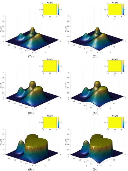
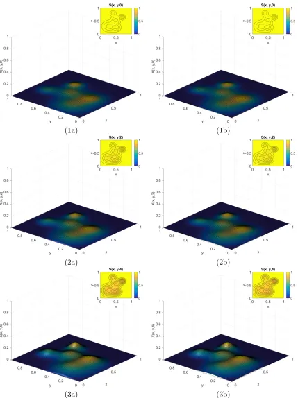
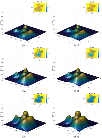
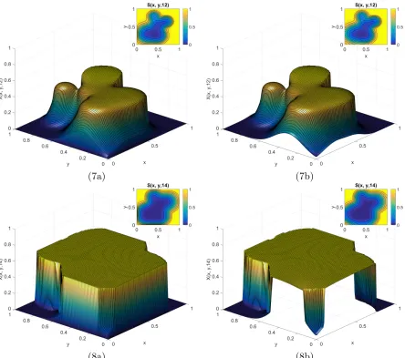
3 Results forE3 . . . 83
7 Concluding Remarks . . . 99
8 Appendix . . . 108
1 Matlab Code . . . 108
List of Figures
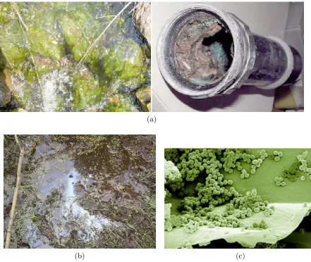
2.1 (a) Biofilm growth on rocks in a stream (USGS) and within a kitchen pipe (MSU Center for Biofilm Engineering). (b) Biofilm phenomena can be caused by bacteria such asThiobacillus ferrooxidans(Iron Bacteria). Bacterial biofilm create oil-like films when they attach themselves to the water surface. Sun-light bounces off the films, giving them an oily appearance. (c) An image from an electron scanning microscope of aStaphylococcus aureus biofilm on a
vascular prosthesis[1]. . . 3
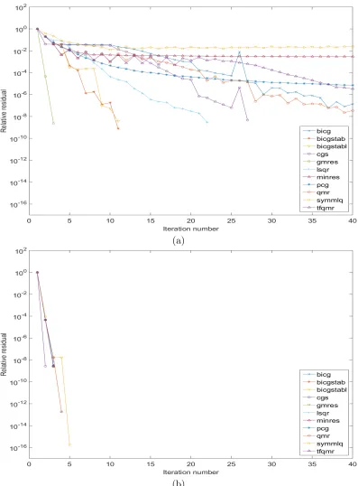
5.1 Plot of residuals vs. iterations of 11 iterative schemes for one time step of E3 (a) without and (b) with preconditioning LU matrix. . . 65
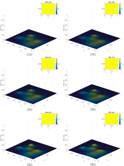
6.1 Time course of E1 for Example 1.1 when t = {0,1,2} with (a) homogeneous Dirichlet and (b) homogeneous Neumann conditions. . . 69
6.2 Continued time course ofE1 for Example 1.1 when t ={3,4,5}. . . 70
6.3 Continued time course ofE1 for Example 1.1 when t ={6,7,8}. . . 71
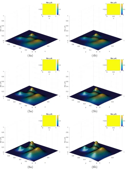
6.4 Time course of E1 for Example 1.2 when t = {0,2,4} with (a) homogeneous Dirichlet and (b) homogeneous Neumann conditions. . . 72
6.5 Continued time course ofE1 for Example 1.2 when t ={6,8,10}. . . 73
6.6 Continued time course ofE1 for Example 1.2 when t ={12,14}. . . 74
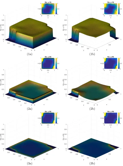
6.7 Time course ofE1 for Example 1.3 when t ={15,20,30}. . . 76
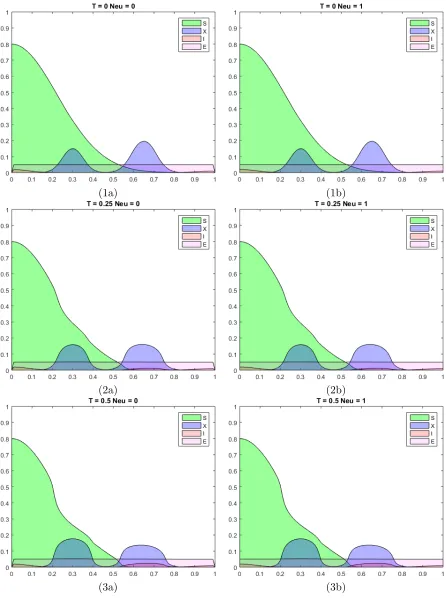
6.8 Time course ofE2 for Example 2.1 when t ={0,0.25,0.5}. . . 78
6.9 Continued course ofE2 for Example 2.1 when t ={0.75,1,1.5}. . . 79
6.10 Continued course of E2 for Example 2.1 when t ={2,5,10}. . . 80
6.11 Time course of E2 for Example 2.2 when t ={0,0.5,1}. . . 84
6.12 Continued course of E2 for Example 2.2 when t ={2,5,10}. . . 85
6.13 Continued course of E2 for Example 2.2 when t ={14,18,22}. . . 86
6.14 Continued course of E2 for Example 2.2 when t ={26,30,40}. . . 87
6.15 Continued course of E2 for Example 2.2 when t ={60,80,100}. . . 88
6.16 Time course of E3 for Example 3.1 when t ={0,0.1,0.2,0.3,0.5,0.7}. . . 90
6.17 Continued course of E3 for Example 3.1 when t ={0.9,1,1.5,2,2.5,3}. . . 91
6.18 Continued course of E3 for Example 3.1 when t ={4,5,6,7,8,9}. . . 92
6.19 Continued course of E3 for Example 3.1 when t ={10,15,20,25,30,35}. . . . 93
6.20 Time course of E3 for Example 3.2 when t ={0,3,6,9,12,15}. . . 95
6.21 Continued course of E3 for Example 3.2 when t ={18,21,24,27,30,33}. . . . 96
List of Symbols
Ω the spatial boundary domain
Ω the closure of the boundary domain Ω
N the set of natural numbers
Z the set of integers
R the set of Euclidean real numbers
R+ the positive reals
Rp p-dimensional Euclidean numbers
x∈Ω x belongs to the set Ω
D: [0,1)→R the function D mapping the interval [0,1) to the reals
× the outer product operator
∪ the set union operator
∇ the gradient operator
∇2 the Laplacian operator
∂
∂t the partial differentiation operator with respect to t Ej biofilm model experiment j ∈ {1,2,3}
LEj length of vectors in experiment Ej. LE1 = 2(M + 1)(N + 1),
LE2 = 4(M + 1), LE3 = 4(M + 1)(N + 1)
aEj the vector a in boldface of lengthLEj
ai the vector element of a where i∈ {1,2, . . . , LEj}
a<e the operators and relations{+,−, <,≤,=,≥, >}on vectors are componentwise so that ai < ei = 1 for alli∈ {1,2, . . . , LEj}
1A the identity (characteristic) function on the set A
Y =Y(x, t) the biofilm function of any state {s, u, S, X, I, E} referring to substrate and biomass forE1, or substrate, active biomass, inert
biomass, and extracellular polymeric substance for E2 and E3,
respectively
Y0
m, Ym,n0 , Ymk, Ym,nk the discrete form of continuous state variables Y(x, t) at node corresponding to Y(t=tk, x=xm, y =yn)
∆z the step size between nodes of z ∈ {x, y}
ψk,±
m,n,z an arbitrary constant at t = tk, x = xm, y = yn where ± indicates a shift by either +1 or−1 in thez ∈ {x, y}dimension (defined in the dissertation during construction of the functions as warranted)
N the set of function solutions that obey Neumann boundary con-ditions
I the identity block matrix
IN the modified identity block matrix defined as needed in the dissertation
Fk,±
m caligraphic capital letters correspond to block matrices of sizes defined in the dissertation. Superscript k represents time step,
±is either of + (−) case where the block matrix is shifted right (left) of the diagonal block in the main matrix, and m is the block row number of the spatial component it represents
YEk,Y
j any one of the diagonal block matrices Y
k ∈ {Ak E1,B
k E1,B
k,Y E3 },
where Y is defined as corresponding to any one of the biofilm state variables as before
Mk
Ej the M-matrix at time t=tk for experiment Ej
W = (Wi,j) an arbitrary matrix where indices are indicated as a subscript corresponding to the ith row and jth column
ρ(Ak) the spectral radius of Ak, defined as the absolute maximum eigenvalue
1
Abstract
In this work, we design a linear, two step implicit finite difference method to approximate the solutions of a biological system that describes the interaction between a microbial colony and a surrounding substrate. Three separate models are analyzed, all of which can be described as systems of partial differential equations (PDE)s with nonlinear diffusion and reaction, where the biological colony grows and decays based on the substrate bioavailability. The systems under investigation are all complex models describing the dynamics of biological films. In view of the difficulties to calculate analytical solutions of the models, we design here a nu-merical technique to consistently approximate the system evolution dynamics, guaranteeing that nonnegative initial conditions will evolve uniquely into new, nonnegative approxima-tions. This property of our technique is established using the theory of M-matrices, which are nonsingular matrices where all the entries of their inverses are positive numbers. We provide numerical simulations to evince the preservation of the nonnegative character of solutions under homogeneous Dirichlet and Neumann boundary conditions. The computational re-sults suggest that the method proposed in this work is stable, and that it also preserves the bounded character of the discrete solutions.
2
Introduction
A biofilm can be described abstractly as a system of prokaryotic and eukaryotic cells at-tached to a surface and embedded in an organic biological matrix. Some of these biofilms have positive effects and have widespread use in industry, environmental preservation, and biomedical applications. Other biofilms have serious detrimental consequences to the envi-ronment, the medical industry, and even efficiency of thermal reactors. In many cases the study of biofilms derives from learning the structure of the independent types of biofilms so as to promote their growth, or in the bad case, limiting or preventing them from forming on the host environment. To this end, both experimental studies and mathematical modeling based on the field results, or using models built through first principles are paramount in their investigation. In this study, we search for suitable mathematical models for simple biofilm structures and then harness the power of the M-matrix to ensure that the model obeys certain presupposed conditions.
biofilms present an emerging link to the disease pathogenesis of many chronic human infec-tions [4]. A higher incidence of biofilms in chronic rhinosinusitis patients suggests a role in its pathogenesis for example [3]. Bacteria are responsible for a range of human diseases that are difficult to clear for a variety of reasons. Research has shown that bacteria can seek pro-tected environments passively by avoiding deadly environments or actively by manipulating their phenotypic expression and gathering in structured biofilm communities [5].
Additionally, many nosocomial infections are assumed to be the result of the presence of pathogenic films in a wide range of medical devices, like catheters and probes used in different hospital services. Biofilms have a major role in implants or devices placed inside the human body, and pose a serious risk for organ transplants. Future researchers have to aim at identifying effective mechanisms for controlling biofilm formation and to develop antimicrobial agents against bacteria in biofilms [6]. As an example, Fungal keratitis is commonly caused by Fusarium species and less commonly by Candida species, the more recent outbreaks of which were associated with contact lens wear and with certain brands of contact lens care solutions where there were formations of biofilms [7]. Biofilms are found within the lungs of patients with chronic pulmonary infarctions and in particular within patients with cystic fibrosis and are the major cause of morbidity and mortality for these patients. Antimicrobial treatment demonstrates a biphasic killing rate, which indicates the presence of a persister population, and a ready supply of nutrient throughout its depth has fewer persister bacteria and hence may be easier to treat than one with less nutrient [8].
(a)
(b) (c)
devoted to the growth and behavior of the more beneficial biofilms [9]. Phototropic biofilms occur on surfaces exposed to light in a range of terrestrial and aquatic environments, and have widespread applications in wastewater treatment, bioremediation, fish feed production, biohydrogen production, and soil improvement [10].
There have been some promising measures to date that show that our knowledge base is increasing. Bacteria survive in nature by forming biofilms on surfaces and most bacteria and fungi are capable of forming them. Biofilms can be prevented in some cases by antibiotic prophylaxis or early aggressive antibiotic therapy and treated by chronic suppressive antibi-otic therapy. Promising strategies include the use of compounds which can easily dissolve the biofilm matrix and quorum sensing inhibitors, which increases biofilm susceptibility to antibiotics and phagocytosis [11]. Phenol is a byproduct of the industrial process of cork manufacturing, and a phenol degrading bacteria immobilized onto residual cork particles is proposed for the remediation of this industrial effluent, known as self-remediation [12]. The first study to observe the reversible redox conversion of cytochrome c552 in viable Geobac-ter sulfurreducens biofilms demonstrates that spectral changes were fully reversible in both positive and negative directions of the scanning potential [13].
Strategies for improving bioremediation efficiency involving genetic engineering to im-prove strains and chemotactic ability, the use of mixed population biofilms and optimization of physiochemical conditions have been studied [14]. Bacterial signal responsive regula-tory circuits have been employed as a platform to design and construct whole cell bacterial biosensors for reporting toxicity, bioremediation, and killing targeted cells [15]. Finally, a down-well aquifer microbial sampling system has been developed using glass wool or Biosep beads as a solid phase support matrix to monitor microbial community dynamics during field bioremediation experiments at Oak Ridge National Laboratory [16].
with polluted stream water and this biological contact oxidation ditch system augmented with the bacteria could be a viable alternative for treating polluted stream water to achieve improved nitrogen removal [17]. Polluted surface water was remediated in a bioreactor using biofilms on filamentous bamboo in batch and continuous flow models [18]. The responses of cultured phototropic biofilms to diverse phosphorus regimes were assessed using a semi continuous flow incubator, and consequently it is proposed that for efficient nutrient removal from wastewaters, biofilms should be regularly removed to continually maintain growth at the initial stages [19].
kinetics. Simpler mathematical forms of the model under investigation possess analytical results which guarantee the existence and uniqueness of positive solutions, and we reference and utilize such results within the current study. However, the exact resolution of such models for experimentally relevant initial conditions is a task which is practically impossible to accomplish.
is represented by an M-matrix, whose properties will be described in the following chapters. As a consequence of its properties, the matrix is nonsingular and the entries of its inverse are all positive numbers, whence the preservation of the positivity of the approximations readily follows.
In this dissertation our focus will be on the solution of the equations governing the spatiotemporal dynamics of three experimental biofilm representations. The choice of equa-tions will be built using first principles and some phenomenological models commonly found in the literature. Specifically, a system of continuous nonlinear diffusion reaction equations will be determined in the background chapter, as well as descriptions of the state variables, meaningful parameters, and simplifications assumed. In the next chapter, we describe the three biofilm systems analytically and move on to creating the finite difference schemes rel-evant to the equations. Once we dissect the three experimental models into their finite difference schemes, we move on to make sure certain criteria are met to establish solutions using M-matrices. The following chapters are devoted to providing the linear finite differ-ence discretization of our mathematical model, along with an equivalent algebraic form of it. Several remarks are stated in order to show that the vector form of our technique is represented by a square matrix which, under suitable conditions on the temporal step-size, is a nonsingular matrix for which all the entries of its inverse are positive numbers. Clearly, these conditions guarantee the preservation of the positivity of the approximations, and make our technique a useful tool in the computational investigation of complex biological films. Motivation for the general diffusion reaction equations and using M-matrices in other fields is also a significant factor in the development of the solution methods. As positivity preserving, bounded solutions are needed by other subjects, the M-matrix solution method is amenable to certain types of these mathematical models as well.
condi-tions possess the necessary property of maintaining strict diagonal dominance by construc-tion, but Neumann conditions require a much more careful treatment. In fact, given certain criteria, we would have to satisfy conditions of strict diagonal dominance which are no longer feasible on the corresponding boundary rows. Upon increasing the spatial dimension from one to two, we increase the number of boundary nodes where strict diagonal dominance cannot hold. The third chapter provides a method to resolve this problem in establishing a weakly chained diagonal dominance for the overall matrix, thereby ensuring that even under Neumann conditions we can still use this M-matrix method.
3
Background
1
Model Development
Starting in the 1970s, several mathematical models were developed to link substrate flux into the biofilm to the fundamental mechanisms of substrate utilization and mass transport. In the 1980s, models still maintained a one dimensional geometry but spatial patterns for several substrates and different types of biomass were added. Today new mathematical models are being developed to provide mechanistic representations for the factors controlling the formation of complex two and three dimensional biofilm morphologies. Features included in these mathematical models usually are motivated by observations made with powerful new tools for observing biofilms in experimental systems.
together into a mass balance equation that contains terms and parameters for each process. Because most biofilms are complex systems, a biofilm model that attempts to capture all the complexity would need to include mass balance equations for all processes occurring in all compartments, continuity and momentum equations for the fluid in all compartments, and defined conditions for all variables at all system boundaries [29]. Below is a general diagram for the system dynamics which we will be using for our analysis:
Net rate of accumulation
of mass of component in the system
= Mass flow of the component into the system − Mass flow of the component out of the system + Rate of production of the component by transformations − Rate of consumption of the component by transformations
Throughout this discussion, we employ the notation R+ to represent the closure of
R+ in the set of the real numbers with the standard topology. We begin with a simple model
that describes the interaction between an active biomass and its substrate. This model corresponds to Experiment 1 (orE1 throughout the discussion), and the case of homogeneous
Dirichlet conditions was published from our research in [30]. Letds and du be positive, real numbers, and let K1, K2, K3 and K4 be nonnegative numbers. Suppose that α and β are
real numbers such that α, β ≥ 1, and let p be a positive integer. Let Ω be a subset of Rp which is open, bounded and connected, and lets and u be real functions defined in Ω×R+
which are twice differentiable in the interior of their domains, and that satisfy the following system of PDEs, for every (x, t)∈Ω×R+:
∂s
∂t(x, t) = d
s∇2s(x, t)−K 1
s(x, t)u(x, t)
K4+s(x, t) ∂u
∂t(x, t) = d
u∇ ·(D(u(x, t))∇u(x, t))−K
2u+K3
s(x, t)u(x, t)
K4+s(x, t) .
Here, the spatial operators ∇ and ∇2 denote, respectively, the gradient/divergence and the
Laplacian operators; meanwhile, the function D: [0,1)→R is given by:
D(f) = f β
(1−f)α (3.1.2)
for every f ∈ [0,1). Appropriate initial/boundary conditions are required and for Dirichlet conditions we additionally impose:
s(x, t) = 1, u(x, t) = 0, ∀x∈∂Ω,∀t≥0,
s(x,0) =s0(x), u(x,0) =u0(x), ∀x∈Ω, (3.1.3)
for suitable functions s0, u0 : Ω→R. In the case of Neumann conditions we have:
ˆ
n· ∇s(x, t) = 0, ˆn· ∇u(x, t) = 0, ∀x∈∂Ω,∀t ≥0,
s(x,0) = s0(x), u(x,0) =u0(x), ∀x∈Ω, (3.1.4)
for suitable functions s0, u0 : Ω→ R.
In the context of the investigation of microbial biology, (3.1.1) describes the dynamics of interaction between a colony of bacteria whose biomass density at the pointx∈Ω and time
t is given by u(x, t), and the corresponding substrate concentration containing the nutrients that are beneficial to the colony which is given by s(x, t). In this case, the parameters
ds, du, K
1, K2, K3 and K4 represent, respectively, the substrate diffusion coefficient, the
Experiment 2 (E2) and Experiment 3 (E3) will focus on the following equations, where
we now subdivide the biomass into three separate components, namely the active biomass
X, inert biomass I, and extracellular polymeric matrix E, where the mass sum total of all biofilm components is U =X+I+E:
∂S
∂t(x, t) =d S∇ ·
(D(U(x, t)∇S(x, t))− µ
YH XS κS+S
+κLκSX
κS+S
+κEκSE
κS+S ∂X
∂t (x, t) =d U∇ ·
(D(U(x, t)∇X(x, t)) + µXS
κS+S
− κLκSX
κS+S
− κIκSX
κS+S ∂I
∂t(x, t) =d U∇ ·
(D(U(x, t)∇I(x, t)) + κIκSX
κS+S ∂E
∂t(x, t) =d U∇ ·
(D(U(x, t)∇E(x, t)) + YEµXS
κS+S
−κEκSE
κS+S
(3.1.5)
HereDis defined as in (3.1.2). With all parameters being defined as nonnegative constants, we takeY to refer to any one of our four state variables{S, X, I, E}, so thatdY refers to the diffusion coefficient for Y (in our description we only use dS anddU as will explained later),
κS is the Monod half saturation constant for the substrate,µis the maximum specific growth rate of active biomass, YH and YE the yield ratios of biomass grown to substrate consumed and EPS formed to substrate consumed, respectively, κL is the biomass decay rate, and κI and κE are the growth coefficients for inert biomass and EPS. We will once again impose Dirichlet boundary conditions such that:
Y(x, t) = 0, ∀x∈∂Ω,∀t ≥0
Y(x,0) =Y0(x) ∀x∈Ω (3.1.6)
and Neumann conditions where:
ˆ
n· ∇Y(x, t) = 0 ∀x∈∂Ω,∀t≥0,
This system of PDEs can be adapted to multiple spatial dimensions, but we will restrict the present study to the spatially one (E2) and two (E3) dimensional cases.
2
Analytical Results
LetF be the real function defined on [0,1) through the expression
F(u) =
Z u
0
vβ
(1−v)αdv. (3.2.8)
Our work is greatly motivated by the next result that establishes conditions under which nonnegative and bounded solutions of (3.1.1) with boundary conditions from (3.1.3) or (3.1.4) exist and are unique; its proof is a direct consequence of Theorems 2.1 and 2.2 of [21] (repeated below):
Proposition 2.1. Let s0 and u0 satisfy the following conditions:
(A) s0 ∈L∞(Ω)∩H1(Ω) and 0≤s0(x)≤1 for every x∈Ω, (B) u0 ∈L∞(Ω) and F ◦u0 ∈H1
0(Ω)
(C) u0(x)≥0 for every x∈Ω, and ku0k
L∞(Ω) <1.
Then, there exists a unique solution of the problem (3.1.1)satisfying the following properties: 1. s, u∈L∞(Ω×R+)∩C(L2(Ω),[0,∞)),
2. s, F ◦u∈L∞(H1(Ω),R+)∩C(L2(Ω),[0,∞)),
3. 0 ≤s(x, t), u(x, t)≤1 for every (x, t)∈Ω×R+, and kuk L∞(Ω×
R+) <1.
(A) the presence of a sharp front of biomass at the fluid/solid transition,
(B) the existence of a threshold of biomass density,
(C) the fact that the biomass spreading is significant only when the biomass concentration is close to the threshold,
(D) the application of reaction kinetics mechanisms in the production of biomass,
(E) the compatibility of the biomass spreading mechanism with hydrodynamics and with nutrient transfer/consumption models.
4
Computational Models Investigated
1
Basic Definitions
We begin with the following definitions in order to discretize the three experiments investi-gated, and will cover the numerical methods and procedures involved in all three experiments at the same time to avoid restatement. We establish the quantities{K, M, N} ∈Z+, our
spa-tial boundary Ωp ∈
Rp for p∈ {1,2}where Ω1 = [a, b] and Ω2 = [a, b]×[c, d],{a, b, c, d} ∈R,
a < b, and c < d. We fix uniform partitions of the intervals [a, b],[c, d] of the form:
a=x0 < x1 <· · ·< xm <· · ·< xM =b (4.1.1)
and
c=y0 < y1 <· · ·< yn <· · ·< yN =d (4.1.2)
for everym∈ {0,1, . . . , M}andn ∈ {0,1, . . . , N}. Let ∆xand ∆yrepresent the spatial step sizes in thexandydirections, respectively, where ∆x= (b−a)/M and ∆y= (d−c)/N. Fix the temporal period of length equal to T ∈R+, and take a uniform partition of the interval
0 =t0 < t1 <· · ·< tk <· · ·< tK =T (4.1.3)
for every k ∈ {0,1, . . . , K}, the norm being ∆t = T /K. The definitions for all three experiments will use these quantities with the restriction of E2 being in only the x spatial
dimension.
We adopt the typical convention for the biomass state variables for all three experi-ments: E1 modeling the interaction of substrate s and active biomass u in Ω2×R+ as skm,n, uk
m,n, E2 in Ω1 ×R+ but with the addition of inert biomass I and EPS E (through the
components Smk, Xmk, Imk, Emk) and E3 in Ω2 ×R+ with Sm,nk , Xm,nk , Im,nk , Em,nk to represent approximations to exact values of S, X, I, and E respectively at the point (xm, yn, tk) for each m ∈ {0,1, . . . , M}, n ∈ {0,1, . . . , N}, and k ∈ {0,1, . . . , K}. Uk
m for E2 is defined as
the sum of the constituent biomass state variables without substrate:
Umk =Xmk +Imk +Emk (4.1.4)
whereas in E3 we define the sum Um,nk as:
Um,nk =Xm,nk +Im,nk +Em,nk (4.1.5)
2
Finite Difference Operators
We make the following definitions to simplify the numerical finite difference method, where
δ+t Ymk = Y k+1 m −Ymk
∆tk
(4.2.6)
The above equation (4.2.6) is a standard forward difference in time operator.
δx±Ymk = Y k
m±1 −Ymk
∆x (4.2.7)
Similarly, (4.2.7) corresponds to the standard forward (backward) difference in space oper-ators.
µ±xYmk = Y k
m±1+Ymk
2 (4.2.8)
(4.2.8) Acts as an averaging operator on the state variables.
±xYmk =D(µ±xUmk)δx±Ymk+1 (4.2.9)
xYmk =
+xYmk +−xYmk
∆x (4.2.10)
Definitions eqs. (4.2.8)–(4.2.10) are operators somewhat more specific to the problem that greatly simplify the finite difference equations.
The definitions for the finite difference operators change only slightly for E1 and
E3, and are included below, with Ym,nk representing any one of {u, s, S, X, I, E} for m ∈
δt+Ym,nk = Y k+1
m,n −Ym,nk ∆tk
(4.2.11)
δx±Ym,nk = Y k
m±1,n−Ym,nk
∆x (4.2.12)
δy±Ym,nk = Y k
m,n±1−Ym,nk
∆y (4.2.13)
µ±xYm,nk = Y k
m±1,n+Ym,nk
2 , µ
± yY
k m,n =
Ym,nk ±1+Ym,nk
2 (4.2.14)
±zYm,nk =D(µ±zUm,nk )δz±Ym,nk+1 (4.2.15)
zYm,nk = +
zYm,nk + − zYm,nk
∆z (4.2.16)
It should be understood that operator eqs. (4.2.11)–(4.2.16) are just eqs. (4.2.6)–(4.2.10) in two spatial dimensions operating on those dimensions separately. Finally we define the second order operators (4.2.17) and (4.2.18):
δx2Ym,nk = Y k
m+1,n−2Ym,nk +Ymk−1,n
δy2Ym,nk = Y k
m,n+1−2Ym,nk +Ym,nk −1
(∆y)2 (4.2.18)
3
Construction of Finite Difference Equations
The fully discretized system of eq. (3.1.1) in E1 now reads as:
δt+skm,n =ds(δx2+δy2)skm,n+1−K1
ukm,nskm,n+1
K4+skm,n
δ+t ukm,n =du(x+y)ukm,n−K2Xm,nk+1+K3
skm,nukm,n+1
K4+skm,n
(4.3.19)
Experiments E2 and E3 corresponding to eq. (3.1.5), which are similar in structure, are both
shown below. For E2 we have:
δt+Smk =dSxSmk −a1
XmkSmk+1 κS+Smk
+a2 Xmk κS+Smk
+a3 Emk κS+Smk
δt+Xmk =dUxXmk +µ
XmkSmk+1 κS+Smk
−a4
Xmk+1 κS+Smk
δt+Imk =dUxImk +a4
Xmk+1 κS+Smk
δt+Emk =dUxEmk +a5
XmkSmk+1 κS+Smk
−a3
Emk+1 κS+Smk
, (4.3.20)
δ+t Sm,nk =dS(x+y)Sm,nk −a1
Xm,nk Sm,nk+1
κS+Sm,nk +a2
Xm,nk
κS+Sm,nk +a3
Em,nk
κS+Sm,nk
δt+Xm,nk =dU(x+y)Xm,nk +µ
Xm,nk Sm,nk+1
κS+Sm,nk
−a4
Xm,nk+1
κS+Sm,nk
δ+t Im,nk =dU(x+y)Im,nk +a4
Xm,nk+1
κS+Sm,nk
δ+t Em,nk =dU(x+y)Em,nk +a5
Xm,nk Sm,nk+1
κS+Sm,nk
−a3
Em,nk+1
κS+Sm,nk
, (4.3.21)
where the nonnegative constants above are simplified as:
a1 = µ YH a2 =κLκS, a3 =κEκS,
a4 =κLκS+κIκS, a5 =YEµ
(4.3.22)
Establishing initial and boundary conditions for all three experiments for simply Dirichlet conditions is relatively easy, and will be used in our initial construction of all the experimental M-matrices. The discrete form of the continuous Dirichlet boundary conditions in eq. (3.1.3), which hold for E1 and E3 with m ∈ {0,1, . . . , M}, n∈ {0,1, . . . , N}, k ∈ {0,1, . . . , K}, and
with Y ∈ {s, u, S, X, I, E}are:
Ym,k0 =Ym,Nk =Y0k,n =YM,nk = 0 (4.3.23)
Equivalently, eq. (3.1.6) of E2 yields the similar conditions:
Neumann boundary conditions will require that the normal derivative to the boundary is 0, so we need to make a suitable approximation. E2 is one dimensional so the approximate
derivative to eq. (3.1.7) in x gives us the conditions for all k∈ {0,1, . . . , K}:
∂Y ∂x
x∈∂Ω
= 0 =⇒ ∂Y
∂x ≈ Yk
1 −Y0k
∆x = 0 =⇒ Y k 1 −Y
k 0 = 0, ∂Y
∂x
x∈∂Ω
= 0 =⇒ ∂Y
∂x ≈
YMk −YMk−1
∆x = 0 =⇒ Y k M −Y
k
M−1 = 0
(4.3.25)
For the two dimensional Neumann boundaries in E1 and E3 for eq. (3.1.7) we have similar
conditions, but we need to take linear combinations of endpoints at the corners:
Ym,k0−Ym,k1 = 0, Ym,Nk −Ym,Nk −1 = 0 ∀m∈ {1,2, . . . , M −1}, Y1k,n−Y0k,n= 0, YM,nk −YMk−1,n = 0 ∀n∈ {1,2. . . , N−1}, and
2Y0k,0−Y0k,1−Y1k,0 = 0,
2Y0k,N −Y0k,N−1−Y1k,N = 0,
2YM,k0−YMk−1,0 −YM,k1 = 0,
2YM,Nk −YMk−1,N−YM,Nk −1 = 0
(4.3.26)
We also require that for all m∈ {0,1, . . . , M} and n ∈ {0,1, . . . , N}, we have the following for E1, E2, and E3:
0≤s0m,n ≤1, 0≤u0m,n <1 (4.3.27)
0≤Sm0 ≤1, 0≤Xm0 <1, 0≤Im0 <1, 0≤Em0 <1,
0≤Sm,n0 ≤1, 0≤Xm,n0 <1, 0≤Im,n0 <1, 0≤Em,n0 <1
Um,n0 =Xm,n0 +Im,n0 +Em,n0 <1 (4.3.29)
This ensures that the nonlinear diffusion mechanism does not attain its infinite discontinuity.
Our overall system will be composed of the iterative solution to a 2(M + 1)(N + 1)× 2(M + 1)(N + 1) M-matrix in E1, a 4(M + 1)× 4(M + 1) M-matrix in E2, and a
4(M + 1)(N + 1)×4(M + 1)(N + 1) M-matrix in E3. After defining the term for each k ∈ {0,1, . . . , K −1}
Rk,Yz =dY ∆tk
(∆z)2, z ∈ {x, y}, Y ∈ {s, u, S, U} (4.3.30)
we can begin to examine the constituent equations row-wise for each state variable in all experiments. We first define the discrete form of the state variables for s(x, y, t) =skm,n and
u(x, y, t) = ukm,n of E1. After some algebraic manipulations, we have:
−Rk,sx skm+1−1,n−Ryk,sskm,n+1−1+φkm,nsm,nk+1−Rk,sy skm,n+1+1−Rk,sx skm+1+1,n =skm,n (4.3.31)
ψm,n,xk,− ukm+1−1,n+ψm,n,yk,− ukm,n+1−1+χkm,num,nk+1+ψm,n,yk,+ ukm,n+1+1+ψm,n,xk,+ ukm+1+1,n =ukm,n (4.3.32)
Here the sets of equations run through allm={1,2, . . . , M−1},n ={1,2, . . . , N−1}, and
φkm,n = 1 + 2Rk,sx + 2Rk,sy +K1∆tk uk
m,n K4 +skm,n
(4.3.33)
ψk,m,n,z± =−Rk,uz D(µ±zukm,n), (4.3.34)
χkm,n = 1−ψk,m,n,x− −ψm,n,yk,− −ψm,n,yk,+ −ψk,m,n,x+ +K2∆tk−K3∆tk
skm,n K4+skm,n
(4.3.35)
Remark 3.1. By inspection, it is easy to see that:
1. Every φkm,n is positive.
2. Every −Rk,s
z and ψk, ±
m,n,z are negative.
3. If we ensure that K3∆tk<1 +K2∆tk, then we have:
χkm,n ≥1 +K2∆tk−K3∆tk sk
m,n K4+skm,n
≥1 +K2∆tk−K3∆tk >0, (4.3.36)
Therefore every χkm,n is positive.
In turn we examine the constituent equations row-wise for the each state variable in E2.
After some algebraic manipulations, we have:
αk,m−Smk+1−1+β k,S m S
k+1 m +α
k,+ m S
k+1 m+1+ζ
k,1 m X
k+1 m +η
k mE
k+1
m =S
k
m (4.3.37)
αmk,−Xmk+1−1+βmk,XXmk+1+αmk,+Xmk+1+1+γmk,1Smk+1 =Xmk (4.3.38)
αmk,−Imk+1−1+βmk,IImk+1+αmk,+Imk+1+1+ζmk,2Xmk+1 =Imk (4.3.39)
αmk,−Emk+1−1+βmk,EEmk+1+αmk,+Emk+1+1+γmk,2Xmk+1 =Emk (4.3.40)
αmk,± =−Rk,Yx D(µ±xUmk) (4.3.41)
βmk,S = 1−αmk,−−αmk,++a1
∆tkXmk κS +Smk
(4.3.42)
βmk,X = 1−αk,m−−αmk,++ a4∆tk
κS+Smk
(4.3.43)
βmk,I = 1−αk,m−−αmk,+ (4.3.44)
βmk,E = 1−αk,m−−αmk,++ a3∆tk
κS+Smk
(4.3.45)
ζmk,1 =− a2∆tk
κS+Smk
(4.3.46)
ηkm =− a3∆tk
κS+Smk
(4.3.47)
γmk,1 =−µ∆tkX
k m κS+Smk
(4.3.48)
ζmk,2 =− a4∆tk
κS+Smk
(4.3.49)
γmk,2 =−a5∆tkX
k m κS+Smk
(4.3.50)
Remark 3.2. By inspection, it is easy to see that:
1. Every αk,±
m is negative.
2. Every ζmk,j, γmk,j, and ηmk are negative.
3. Every βk,Y
m is positive.
Finally, for E3 and just an expansion in spatial dimensions of E2, we have:
αk,m,n,x− Smk+1−1,n+αk,m,n,y− Sm,nk+1−1+βm,nk,SSm,nk+1+αk,m,n,y+ Sm,nk+1+1
+αk,m,n,x+ Smk+1+1,n+ζm,nk,1Xm,nk+1+ηm,nk Em,nk+1 =Sm,nk (4.3.51)
αk,m,n,x− Xmk+1−1,n+α k,− m,n,yX
k+1 m,n−1+β
k,X m,nX
k+1 m,n +α
k,+ m,n,yX
k+1 m,n+1
αk,m,n,x− Imk+1−1,n+α k,− m,n,yI
k+1 m,n−1+β
k,I m,nI
k+1 m,n +α
k,+ m,n,yI
k+1 m,n+1
+αk,m,n,x+ Imk+1+1,n+ζm,nk,2 Xm,nk+1 =Im,nk (4.3.53)
αk,m,n,x− Emk+1−1,n+αk,m,n,y− Em,nk+1−1+βm,nk,EEm,nk+1+αk,m,n,y+ Em,nk+1+1
+αk,m,n,x+ Emk+1+1,n+γm,nk,2 Xm,nk+1 =Em,nk (4.3.54)
Constants are defined below.
αk,m,n,z± =−Rk,Yz D(µ±zUm,nk ) (4.3.55)
βm,nk,S = 1−αk,m,n,x− −αm,n,xk,+ −αk,m,n,y− −αk,m,n,y+ +a1
∆tkXm,nk κS+Sm,nk
(4.3.56)
βm,nk,X = 1−αk,m,n,x− −αk,m,n,x+ −αk,m,n,y− −αk,m,n,y+ + a4∆tk
κS+Sm,nk
(4.3.57)
βm,nk,I = 1−αk,m,n,x− −αm,n,xk,+ −αk,m,n,y− −αk,m,n,y+ (4.3.58)
βm,nk,E = 1−αk,m,n,x− −αk,m,n,x+ −αk,m,n,y− −αk,m,n,y+ + a3∆tk
κS+Sm,nk
(4.3.59)
ζm,nk,1 =− a2∆tk
κS+Sm,nk
(4.3.60)
ηm,nk =− a3∆tk
κS+Sm,nk
(4.3.61)
γm,nk,1 =−µ∆tkX
k m,n κS+Sm,nk
(4.3.62)
ζm,nk,2 =− a4∆tk
κS+Sm,nk
(4.3.63)
γm,nk,2 =−a5∆tkX
k m,n κS+Sm,nk
(4.3.64)
Remark 3.3. By inspection, it is easy to see that:
1. Every αk,±
m,n,z is negative.
2. Every ζk,j
m,n, γm,nk,j , and ηm,nk are negative.
4
Assembly of M-matrices
Now that we have established the equations corresponding to each of our experiments, we are ready to assemble the matrices which will in turn be used to progress the evolution of the biofilm complexes forward in time. Up to this point we have assembled the main coefficients out of the finite difference equations, but have not indicated the functional dependence of them on the previous state of the model. The definitions below serve to describe the ordering of the nodal points as vectors, and in our matrix definitions and vector approximations it should be implicitly understood that there is a functional dependence on the preceding state vector. This is only for notational convenience. As before we start with E1. Let k be an
element of {0,1, . . . , K}, and let sk
E1 and u
k
E1 be the ordered vector approximations of the
state variables at time tk, defined as:
skE
1 = (s
k 0,0, s
k
0,1, . . . , s k 0,N, s
k 1,0, s
k
1,1, . . . , s k
1,N, . . . , s k M,0, s
k
M,1, . . . , s k
M,N) (4.4.65) ukE1 = (uk0,0, uk0,1, . . . , uk0,N, uk1,0, uk1,1, . . . , uk1,N, . . . , uM,k 0, ukM,1, . . . , ukM,N) (4.4.66)
Letvk E1 = (s
k E1|u
k E1)
t, and further let s0
E1 and u
0
E1 be defined as:
s0E
1 = (0,0, . . . ,0 | {z }
N+1 entries
,0, s01,1, . . . , s01,N−1,0
| {z }
N+1 entries
, . . . ,
. . . ,0, s0M−1,1, . . . , s0M−1,N−1,0
| {z }
N+1 entries
,0,0, . . . ,0
| {z }
N+1 entries
u0E1 = (0,0, . . . ,0
| {z }
N+1 entries
,0, u01,1, . . . , u01,N−1,0
| {z }
N+1 entries
, . . . ,
. . . ,0, u0M−1,1, . . . , u0M−1,N−1,0
| {z }
N+1 entries
,0,0, . . . ,0
| {z }
N+1 entries
) (4.4.68)
Finally we let v0 E1 = (s
0 E1|u
0 E1)
t. By construction it should be noted that bothvk
E1 andv
0 E1 are
length 2(M+ 1)(N+ 1) vectors. Each matrix and submatrix will be assigned its own unique capital letter and given a reference number for the proofs to follow. As we will be defining block matrices based on not only eqs. (4.3.31) and (4.3.32), we must include the boundary conditions on the values corresponding to indices not contained in the interior of the domain as indicated in (4.3.26). We will use the indicator function defined as follows to denote the difference in the matrix if it is used for the Dirichlet or the Neumann conditions, where N refers to the set of functions whose closed boundary obeys Neumann conditions, and if not they obey Dirichlet conditions:
1N(∂Ω) :=
(
1 if ∂Ω∈N ,
0 if ∂Ω∈/ N . (4.4.69)
Additionally, we letI represent the identity matrix of size (N+1)×(N+1) andIN represent the modified identity matrix of size (N + 1)×(N + 1) defined below:
IN =
1 +1N(∂Ω) −1N(∂Ω) 0 · · · 0 0 0
0 1 0 · · · 0 0 0
0 0 1 · · · 0 0 0
..
. ... ... . .. ... ... ...
0 0 0 · · · 1 0 0
0 0 0 · · · 0 1 0
0 0 0 · · · 0 −1N(∂Ω) 1 +1N(∂Ω)
For every m ∈ {1,2, . . . , M −1} and every k ∈ {0,1, . . . , K}, let Ck and Dk
m be the diagonal and tridiagonal matrices of size (N+ 1)×(N + 1) given by
Ck=
0 0 0 0 · · · 0 0 0
0 −Rk,sx 0 0 · · · 0 0 0
0 0 −Rk,s
x 0 · · · 0 0 0
0 0 0 −Rk,s
x · · · 0 0 0
..
. ... ... ... . .. ... ... ...
0 0 0 0 · · · −Rk,sx 0 0
0 0 0 0 · · · 0 −Rk,s
x 0
0 0 0 0 · · · 0 0 0
(4.4.71) and
Dmk =
1 −1N(∂Ω) 0 0 · · · 0 0 0
−Rk,sy φkm,1 −Rk,sy 0 · · · 0 0 0
0 −Rk,sy φkm,2 −Rk,sy · · · 0 0 0
0 0 −Rk,sy φkm,3 · · · 0 0 0
..
. ... ... ... . .. ... ... ...
0 0 0 0 · · · φkm,N−2 −Ryk,s 0
0 0 0 0 · · · −Ryk,s φkm,N−1 −Rk,sy
0 0 0 0 · · · 0 −1N(∂Ω) 1
(4.4.72)
Now we define the square matrix Ak
E1 as the block matrix of size (M + 1)(N + 1)×(M +
Ak E1 =
IN −1N(∂Ω)I 0 0 · · · 0 0 0
Ck Dk
1 Ck 0 · · · 0 0 0
0 Ck Dk
2 Ck · · · 0 0 0
0 0 Ck Dk
3 · · · 0 0 0
..
. ... ... ... . .. ... ... ...
0 0 0 0 · · · Dk
M−2 Ck 0
0 0 0 0 · · · Ck Dk
M−1 Ck
0 0 0 0 · · · 0 −1N(∂Ω)I IN
(4.4.73)
In that same fashion, we create the submatrices Fk,±
m and Gmk of size (N + 1)×(N + 1)
Fmk,± =
0 0 0 0 · · · 0 0 0
0 ψm,k,±1,x 0 0 · · · 0 0 0
0 0 ψm,k,±2,x 0 · · · 0 0 0
0 0 0 ψm,k,±3,x · · · 0 0 0
..
. ... ... ... . .. ... ... ...
0 0 0 0 · · · ψm,Nk,±−2,x 0 0
0 0 0 0 · · · 0 ψm,Nk,±−1,x 0
0 0 0 0 · · · 0 0 0
(4.4.74) and Gk m =
1 −1N(∂Ω) 0 · · · 0 0 0
ψm,k,−1,y χk
m,1 ψ k,+
m,1,y · · · 0 0 0
0 ψk,m,−2,y χk
m,2 · · · 0 0 0
..
. ... ... . .. ... ... ... 0 0 0 · · · χkm,N−2 ψk,m,N+−2,y 0 0 0 0 · · · ψm,Nk,−−1,y χkm,N−1 ψm,Nk,+−1,y
0 0 0 · · · 0 −1N(∂Ω) 1
(4.4.75)
Once again, we define the square matrix Bk
E1 as the block matrix of size (M + 1)(N + 1)×
BEk1 =
IN −1N(∂Ω)I 0 0 · · · 0 0 0
F1k,− Gk
1 F
k,+
1 0 · · · 0 0 0
0 F2k,− Gk
2 F
k,+
2 · · · 0 0 0
0 0 F3k,− Gk
3 · · · 0 0 0
..
. ... ... ... . .. ... ... ...
0 0 0 0 · · · Gk
M−2 F k,+
M−2 0
0 0 0 0 · · · FMk,−−1 Gk
M−1 F
k,+ M−1
0 0 0 0 · · · 0 −1N(∂Ω)I IN
(4.4.76)
Now, for everyk ∈ {0,1, . . . , K −1}, we define the block matrix Mk
E1 of size 2(M+ 1)(N+
1)×2(M+ 1)(N+ 1) where zero entries are matrices of size (M+ 1)(N+ 1)×(M+ 1)(N+ 1):
Mk E1 =
Ak E1 0
0 Bk E1
(4.4.77)
With this nomenclature for E1 we can write our continuous eq. (3.1.1) as a finite difference
approximation in eq. (4.3.19) using a matrix equation with Mk
E1 and v
k
E1, keeping in mind
our first step would use v0
E1 on the right hand side (and making sure this initial condition
vector’s elements are all indeed positive and bounded by one):
MkE1vkE+1
1 =v
k
E1 (4.4.78)
To reiterate what was said on the matrix equation, we assume that we have a linear mapping (Mk
E1)
−1 : vk E1 → v
k+1
E1 As the inverse M-matrix only depends on the values of v
k
E1 and we
prove that we do indeed have an M-matrix throughout the dissertation, we are ensured that the solution exists whence we have a valid vk
E1.
its corresponding inverse on the previous state vector supplied. For E2, let YEk2 be any
of {Sk E2, X
k E2, I
k E2, E
k
E2} the ordered vector approximations of the state variables at time tk,
defined as:
SkE2 = (S0k, S1k, . . . , SMk ) (4.4.79)
XkE2 = (X0k, X1k, . . . , XMk ) (4.4.80)
IkE
2 = (I
k 0, I
k 1, . . . , I
k
M) (4.4.81)
EkE2 = (E0k, E1k, . . . , EMk ) (4.4.82)
Letvk E2 = (S
k E2|X
k E2|I
k E2|E
k E2)
t, and further let S0 E2, X
0 E2, I
0
E2 and E
0
E2 be defined as:
S0E
2 = (0, S
0
1, . . . , S 0 M−1,0
| {z }
M+1 entries
) (4.4.83)
X0E2 = (0, X10, . . . , XM0 −1,0
| {z }
M+1 entries
) (4.4.84)
I0E2 = (0, I10, . . . , IM0 −1,0
| {z }
M+1 entries
) (4.4.85)
E0E
2 = (0, E
0
1, . . . , E 0 M−1,0
| {z }
M+1 entries
) (4.4.86)
Finally we let v0
E2 = (S
0 E2|X
0 E2|I
0 E2|E
0 E2)
t. By construction it should be noted that both vk E2
The case of assembling the matrices for E2 is slightly easier. Defining a collection of
matrices of size (M + 1)×(M + 1) for each k ∈ {0,1, . . . , K −1}, and letting Y represent any of the functions S, X, I, E, we define the tridiagonal matrix
BEk,Y
2 =
1 −1N(∂Ω) 0 0 · · · 0 0 0
αk,1− β1k,Y α1k,+ 0 · · · 0 0 0
0 αk,2− β2k,Y αk,2+ · · · 0 0 0
0 0 α3k,− β3k,Y · · · 0 0 0
..
. ... ... ... . .. ... ... ... 0 0 0 0 · · · βMk,Y−2 αk,M+−2 0 0 0 0 0 · · · αk,M−−1 βMk,Y−1 αk,M+−1
0 0 0 0 · · · 0 −1N(∂Ω) 1
(4.4.87)
We define also the diagonal matrices with the same size as Bk,YE
2 forj ∈ {1,2},
Hk E2 =
0 0 0 · · · 0 0
0 η1k 0 · · · 0 0 0 0 ηk
2 · · · 0 0
..
. ... ... . .. ... ... 0 0 0 · · · ηk
M−1 0
0 0 0 · · · 0 0
, (4.4.88) and
ZEk,j
2 =
0 0 0 · · · 0 0
0 ζ1k,j 0 · · · 0 0 0 0 ζ2k,j · · · 0 0
..
. ... ... . .. ... ... 0 0 0 · · · ζMk,j−1 0
0 0 0 · · · 0 0
, Γk,jE
2 =
0 0 0 · · · 0 0
0 γ1k,j 0 · · · 0 0 0 0 γ2k,j · · · 0 0
..
. ... ... . .. ... ... 0 0 0 · · · γk,jM−1 0
0 0 0 · · · 0 0
Now, for every k ∈ {0,1, . . . , K −1}, we define the block matrix Mk
E2 of size 4(M + 1)×
4(M+ 1) where zero entries are matrices of size (M + 1)×(M + 1):
Mk E2 =
Bk,SE
2 Z
k,1
E2 0 H
k E2
Γk,E1
2 B
k,X
E2 0 0
0 ZEk,22 BEk,I2 0 Γk,E2
2 0 0 B
k,E E2 (4.4.90)
Once again we can representE2 from the continuous to discrete eqs. (3.1.5) and (4.3.20) as a
matrix evolution equation identical in form to eq. (4.4.78) ofE1 but with matrix and vectors
defined to reflect eqs. (3.1.5) and (4.3.20):
Mk E2v
k+1 E2 =v
k
E2 (4.4.91)
E3 uses the same ideas from both of these methods in the sense that it derives the
construction from E1 but the number of state variables from E2. Let k be an element of {0,1, . . . , K}, and let Sk
E3, X
k E3, I
k
E3, and E
k
E3 be the ordered vector approximations of the
state variables at time tk, defined as:
SkE
3 = (S
k 0,0, S
k
0,1, . . . , S k 0,N, S
k 1,0, S
k
1,1, . . . , S k
1,N, . . . , S k M,0, S
k
M,1, . . . , S k
M,N) (4.4.92) XEk3 = (X0k,0, X0k,1, . . . , X0k,N, X1k,0, X1k,1, . . . , X1k,N, . . . , XM,k 0, XM,k 1, . . . , XM,Nk ) (4.4.93)
IEk3 = (I0k,0, I0k,1, . . . , I0k,N, I1k,0, I1k,1, . . . , I1k,N, . . . , IM,k 0, IM,k 1, . . . , IM,Nk ) (4.4.94)
EkE
3 = (E
k 0,0, E
k
0,1, . . . , E k 0,N, E
k 1,0, E
k
1,1, . . . , E k
1,N, . . . , E k M,0, E
k
M,1, . . . , E k
M,N) (4.4.95)
S0E3 = (0,0, . . . ,0
| {z }
N+1 entries
,0, S10,1, . . . , S10,N−1,0
| {z }
N+1 entries
, . . . ,
. . . ,0, SM0 −1,1, . . . , SM0 −1,N−1,0
| {z }
N+1 entries
,0,0, . . . ,0
| {z }
N+1 entries
) (4.4.96)
X0E3 = (0,0, . . . ,0
| {z }
N+1 entries
,0, X10,1, . . . , X10,N−1,0
| {z }
N+1 entries
, . . . ,
. . . ,0, XM0 −1,1, . . . , XM0 −1,N−1,0
| {z }
N+1 entries
,0,0, . . . ,0
| {z }
N+1 entries
) (4.4.97)
I0E3 = (0,0, . . . ,0
| {z }
N+1 entries
,0, I10,1, . . . , I10,N−1,0
| {z }
N+1 entries
, . . . ,
. . . ,0, IM0 −1,1, . . . , IM0 −1,N−1,0
| {z }
N+1 entries
,0,0, . . . ,0
| {z }
N+1 entries
) (4.4.98)
E0E3 = (0,0, . . . ,0
| {z }
N+1 entries
,0, E10,1, . . . , E10,N−1,0
| {z }
N+1 entries
, . . . ,
. . . ,0, EM0 −1,1, . . . , EM0 −1,N−1,0
| {z }
N+1 entries
,0,0, . . . ,0
| {z }
N+1 entries
) (4.4.99)
Finally we let v0
E3 = (S
0 E3|X
0 E3|I
0 E3|E
0 E3)
t. By construction it should be noted that both vk E3
To create the M-matrix corresponding to eq. (4.3.21) for E3 we start by observing
that a grouping of (N+ 1)×(N+ 1) submatrices will correspond to the discretized y index
n. For every m ∈ {1, . . . , M −1}, every k ∈ {0,1, . . . , K}, z = {x, y}, and Y representing any of the functions S, X, I, E, we define Fk,±
m and Gmk,Y as:
Fk,±
m =
0 0 0 0 · · · 0 0 0
0 αm,k,±1,x 0 0 · · · 0 0 0
0 0 αk,m,±2,x 0 · · · 0 0 0
0 0 0 αk,m,±3,x · · · 0 0 0
..
. ... ... ... . .. ... ... ...
0 0 0 0 · · · αk,m,N±−2,x 0 0
0 0 0 0 · · · 0 αk,m,N±−1,x 0
0 0 0 0 · · · 0 0 0
, (4.4.100) and Gk,Y m =
1 −1N(∂Ω) 0 · · · 0 0 0
αk,m,−1,y βm,k,Y1 αm,k,+1,y · · · 0 0 0 0 αk,m,−2,y βm,k,Y2 · · · 0 0 0
..
. ... ... . .. ... ... ... 0 0 0 · · · βm,Nk,Y −2 αk,m,N+−2,y 0 0 0 0 · · · αk,m,N− −1,y βm,Nk,Y −1 αk,m,N+ −1,y
0 0 0 · · · 0 −1N(∂Ω) 1
(4.4.101)
Next we construct the block matricesBEk,Y
3 of size (M + 1)(N + 1)×(M + 1)(N + 1), where
Bk,YE 3 =
IN −1N(∂Ω)I 0 0 · · · 0 0 0
F1k,− G1k,Y F1k,+ 0 · · · 0 0 0
0 F2k,− G2k,Y F2k,+ · · · 0 0 0
0 0 F3k,− G3k,Y · · · 0 0 0
..
. ... ... ... . .. ... ... ...
0 0 0 0 · · · GMk,Y−2 FMk,+−2 0
0 0 0 0 · · · FMk,−−1 GMk,Y−1 FMk,+−1
0 0 0 0 · · · 0 −1N(∂Ω)I IN
(4.4.102)
In this same fashion, for every m∈ {1, . . . , M −1}, and every k ∈ {0,1, . . . , K}, we construct the (N + 1)×(N + 1) diagonal matrices Pk,j
m ,Qk,jm , and Tmk for j ∈ {1,2}:
Pk,j m =
0 0 0 0 · · · 0 0 0
0 ζm,k,j1 0 0 · · · 0 0 0
0 0 ζm,k,j2 0 · · · 0 0 0
0 0 0 ζm,k,j3 · · · 0 0 0
..
. ... ... ... . .. ... ... ... 0 0 0 0 · · · ζm,Nk,j −2 0 0 0 0 0 0 · · · 0 ζm,Nk,j −1 0
0 0 0 0 · · · 0 0 0
, (4.4.103) Qk,j m =
0 0 0 0 · · · 0 0 0
0 γm,k,j1 0 0 · · · 0 0 0
0 0 γm,k,j2 0 · · · 0 0 0
0 0 0 γm,k,j3 · · · 0 0 0
..
. ... ... ... . .. ... ... ... 0 0 0 0 · · · γm,Nk,j −2 0 0 0 0 0 0 · · · 0 γm,Nk,j −1 0
0 0 0 0 · · · 0 0 0
Tk m =
0 0 0 0 · · · 0 0 0
0 ηk
m,1 0 0 · · · 0 0 0
0 0 ηk
m,2 0 · · · 0 0 0
0 0 0 ηk
m,3 · · · 0 0 0
..
. ... ... ... . .. ... ... ...
0 0 0 0 · · · ηk
m,N−2 0 0
0 0 0 0 · · · 0 ηk
m,N−1 0
0 0 0 0 · · · 0 0 0
. (4.4.105)
Similarly we create the (M+ 1)(N+ 1)×(M+ 1)(N+ 1) block matricesZEk,j
3 , Γ
k,j
E3, andH
k E3
where the zero entries below are all (N + 1)×(N + 1) submatrices:
ZEk,j
3 =
0 0 0 0 · · · 0 0 0
0 P1k,j 0 0 · · · 0 0 0
0 0 P2k,j 0 · · · 0 0 0
0 0 0 P3k,j · · · 0 0 0
..
. ... ... ... . .. ... ... ...
0 0 0 0 · · · PMk,j−2 0 0
0 0 0 0 · · · 0 PMk,j−1 0
0 0 0 0 · · · 0 0 0
, (4.4.106)
Γk,jE
3 =
0 0 0 0 · · · 0 0 0
0 Qk,j1 0 0 · · · 0 0 0
0 0 Qk,j2 0 · · · 0 0 0
0 0 0 Qk,j3 · · · 0 0 0
..
. ... ... ... . .. ... ... ...
0 0 0 0 · · · Qk,jM−2 0 0
0 0 0 0 · · · 0 Qk,jM−1 0
0 0 0 0 · · · 0 0 0
Hk E3 =
0 0 0 0 · · · 0 0 0
0 Tk
1 0 0 · · · 0 0 0
0 0 Tk
2 0 · · · 0 0 0
0 0 0 Tk
3 · · · 0 0 0
..
. ... ... ... . .. ... ... ...
0 0 0 0 · · · Tk
M−2 0 0
0 0 0 0 · · · 0 Tk
M−1 0
0 0 0 0 · · · 0 0 0
. (4.4.108)
Finally we construct the entire 4(M + 1)(N + 1)×4(M + 1)(N + 1) block matrix
Mk
E3 where zero entries are matrices of size (M + 1)(N + 1)×(M+ 1)(N+ 1):
Mk E3 =
Bk,SE
3 Z
k,1
E3 0 H
k E3
Γk,E1
3 B
k,X
E3 0 0
0 ZEk,2
3 B
k,I
E3 0
Γk,E2
3 0 0 B
k,E E3 (4.4.109)
We can now write our finite difference method as before in eqs. (4.4.78) and (4.4.91):
MkE3vkE+1
3 =v
k
E3 (4.4.110)
5
Criteria to Ensure M-matrices
Up until this point, despite a few remarks, we have not spent any time establishing the requirements for there to be viable solutions to the finite difference systems previously men-tioned for experiments E1 through E3. This section will be devoted to the task of ensuring
Lemma 5.1. [Fujimoto and Ranade (2004)] Every M-matrix is invertible, and the entries of its inverse are all positive real numbers. The necessary requirements for an M-matrix are:
(A) All entries on the diagonal must be positive.
(B) All off-diagonal entries must be nonpositive.
(C) The matrix must be strictly diagonally dominant.
In light of Lemma 5.1, we need to show that each matrix Mk E1,M
k E2,M
k
E3 described
in eqs. (4.4.77), (4.4.90) and (4.4.109) satisfies the requirements (A) (B), and (C) above. The conditions (A) and (B) are easy to show and will be described below in a series of remarks combined with ones made previously. Condition (C) however, the requirement of strict diagonal dominance, cannot be shown for any matrix with Neumann conditions. However, there is a weaker requirement for a square matrix to be an M-matrix which we will prove in the following section. The requirement is due to properties shared with the so called weakly chained diagonally dominant (WCDD) matrices for which strictly diagonally dominant matrices are a subclass [32, 33]. Essentially (and to be described completely further down), an L-matrix which possesses the property of WCDD is an M-matrix. The requirement for an L-matrix is that (A) and (B) are satisfied.
We begin with establishing (A) and (B) for all experiments. We see that for the first and last (N + 1) rows corresponding to the block matrices Ak
E1, B
k
E1, and B
k,Y
E3 , we have one
or two on the diagonal which is obviously positive. Every other off diagonal entry on the top and bottom (N + 1) rows for each of Ak
E1, B
k
E1, and B
k,Y
E3 are -1 (if there are Neumann
conditions) or 0, corresponding to Dirichlet conditions.
Remark 5.2. Recall that the common convention for labeling indexes of matrices uses the
natural numbers. By inspection, it is easy to see that for all boundary conditions we have