What Elasticity of the Matching Function
is consistent with U.S. Aggregate Labor Market Data?
Bj¨orn Br¨
ugemann
∗July 2008
Abstract
The elasticity of the matching function is a key parameter of the search and matching model. There is disagreement which value of this elasticity is appropriate in the context of studying the cyclical behavior of the U.S. labor market. Shimer (2005) obtains an estimate of 0.28 by regressing the job finding probability on the vacancy-unemployment ratio. Mortensen and Nagyp´al (2007) infer a value of 0.54 from the slope of the Beveridge curve. Both approaches rely on assumptions that are problematic. After addressing these problems, both approaches yield estimates between 0.37 and 0.46.
Keywords:
The elasticity of the matching function is a key parameter of the search and matching
model. There is disagreement which value of this elasticity is appropriate in the context
of studying the cyclical behavior of the U.S. labor market. Shimer (2005) obtains an
estimate of 0.28 by regressing the job finding probability on the vacancy-unemployment
ratio. Mortensen and Nagyp´al (2007) infer a value of 0.54 from the slope of the Beveridge
curve. Both approaches rely on assumptions that are problematic. After addressing these
problems, both approaches yield estimates between 0.37 and 0.46.
1
Environment
Time is continuous. There is a unit mass of ex ante identical infinitely lived workers
participating in the labor market. At a point in time one of these workers is either employed
or unemployed. There are no transitions between participation and non-participation.
The process by which unemployed workers find jobs is modeled as a matching technology.
Specifically, the flow of newly employed workers is given bym(u, v) whereu is the number
of unemployed workers, v is the number of vacancies, and m is a constant returns to scale
matching function. Throughout it is assumed that the functional form of the matching
function is Cobb-Douglas
m(u, v) = µu1−ηvη.
Define the vacancy-unemployment ratioθ ≡ vu. The arrival rate of jobs from the perspective
of a worker is m(u,vu ) and can be written as a function of the v-uratio θ:
f(θ)≡m(1, θ) =µθη. (1)
This arrival rate is referred to as the job finding rate.
Employed workers exit from employment into unemployment with time varying arrival
rate xt. This arrival rate is referred to as theemployment exit rate. There is no on-the-job
Table 1: Standard Deviations and Correlations
˜
u e˜ v˜ ˜θ f˜ F˜ x˜ X˜
St. dev. 0.190 0.014 0.202 0.382 0.162 0.118 0.075 0.076
˜
u 1 −0.735 −0.894 −0.972 −0.954 −0.949 0.709 0.709
˜
e 1 0.800 0.789 0.775 0.784 −0.397 −00.397
˜
v 1 0.975 0.893 0.897 −0.684 −0.684
Corr. ˜θ 1 0.948 0.948 −0.715 −0.715
˜
f 1 0.999 −0.584 −0.584
˜
F 1 −0.574 −0.574
˜
x 1 1
˜
X 1
2
U.S. Aggregate Labor Market Data
In this section I briefly summarize the data used by Shimer. Mortensen and Nagyp´al
rely on the same data. The raw data consists of four monthly time series from January
1951 to January 2004. The first three are constructed by the BLS from the CPS: the
level of unemployment ut, the level of civilian employment et, and the number of workers
unemployed for 0 to 4 weeksust. The fourth is the Conference Board help-wanted advertising
index vt, used as a proxy for vacancies.
Define the job finding probability Ft as the probability that a worker unemployed at
time t does not remain unemployed throughout until time t+ 1. If the job finding rate is
constant atft betweentand t+ 1, then under the assumptions of Section 1 the job finding
probability is given by Ft = 1−e−ft. Similarly, define the employment exit probability Xt
as the probability of a worker employed at timetexiting into unemployment between tand
t+ 1. Again, if the employment exit rate is constant at xt during this time interval, then
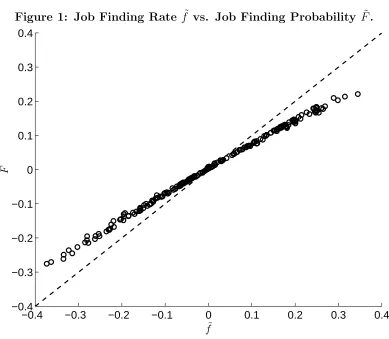
Figure 1: Job Finding Rate f˜vs. Job Finding Probability F˜.
−0.4 −0.3 −0.2 −0.1 0 0.1 0.2 0.3 0.4
−0.4 −0.3 −0.2 −0.1 0 0.1 0.2 0.3 0.4
˜
f ˜F
while the employment exit probability is very well approximated by
Xt=
us t+1 et 1− 12Ft
.
Having measured the two probabilities, measures of the corresponding rates are obtained
through the relationships ft=−log(1−Ft) and xt=−log(1−Xt).
For the following analysis all time series are transformed as follows. First, quarterly
series are constructed as averages of monthly values. Second, logarithms are taken.
Fi-nally, the series are detrendend using a Hodrick-Prescott filter with smoothing parameter
105. If y is the original monthly series, let ˜y denote the time series resulting from these
Table 2: Shimer’s approach
(1) (2)
left hand side F˜ f˜
right hand side ˜θ ˜θ
direct regression 0.292 (0.007) 0.401 (0.009)
reverse regression 0.325 (0.008) 0.447 (0.010)
R2 0.899 0.898
NOTE.– Standard errors in parentheses.
3
Shimer’s (2005) approach.
Equation (1) implies1
˜
ft =η˜θt.
Shimer’s approach is to estimate η from this relationship. He implements this approach
using ˜Ft as a proxy for ˜ft, and obtains an estimate of 0.28. Replicating this regression,
I obtain the estimate 0.29. Using ˜Ft as a proxy for ˜ft is not innocuous, however. Figure
1 plots ˜F against ˜f. The relationship is approximately linear over the relevant range, so
the correlation is near one. Importantly, the relative standard deviation is 0.73. Another
way to see that F is less variable than f is to compute the elasticity of F with respect
to f, given by e−ff
1−e−f. Evaluating this expression at the mean of f, which is 0.61, this
computation also yields 0.73. Intuitively, at low levels of the job finding rate f, doubling
this rate also roughly doubles the probability of finding a job. But if the level of f is high,
then the worker is already very likely to find a job, so doubling the job finding rate can no
longer double the job finding probability.
This discussion implies that regressing ˜ftonθtwill yield a coefficient of 00..2973 = 0.4 where
0.29 is the coefficient from regressing ˜F on ˜θ, and 0.73 is the relative standard deviation of
˜
Figure 2: Time Series of f˜and x˜+ ˜e−u˜.
1955 1960 1965 1970 1975 1980 1985 1990 1995 2000 −0.5 −0.4 −0.3 −0.2 −0.1 0 0.1 0.2 0.3 0.4 0.5 t ˜ f ˜
s+ ˜e−u˜
reverse regression of ˜θ on ˜f, so in Table 2 I report both. For the corrected version of the
approach, direct and reverse regression together suggest the range [0.4,0.45] for η.
4
Mortensen and Nagyp´
al’s approach
If the job finding rate and the employment exit rate remain constant atfandx, respectively,
then the unemployment rate u
u+e will converge to x
x+f. Mortensen and Nagyp´al’s approach
is based on the following observation made by Shimer (2007): due to the large empirical
values off andx, adjustment to x
x+f is very rapid, with the consequence that x
x+f provides
an excellent approximation of u
u+e. Taking this relationship with equality u u+e =
x x+f and
substituting the matching function yields
u u+e =
x
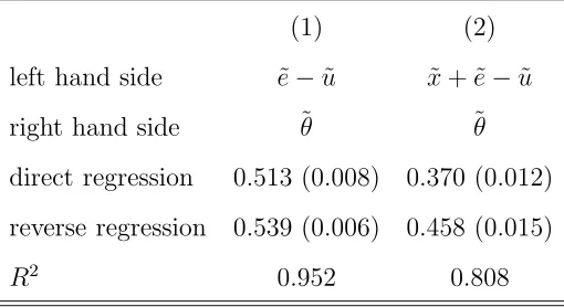
Table 3: Mortensen and Nagyp´al Approach
(1) (2)
left hand side e˜−u˜ x˜+ ˜e−u˜
right hand side ˜θ ˜θ
direct regression 0.513 (0.008) 0.370 (0.012)
reverse regression 0.539 (0.006) 0.458 (0.015)
R2 0.952 0.808
NOTE.– Standard errors in parentheses.
This formula suggests that η can be estimated using data on u, e, v and x. Moreover,
Mortensen and Nagyp´al discuss estimation of the matching function elasticity in the context
of a model with a constant employment exit rate. Under the restriction of a constant
employment exit rate, equation (2) permits estimation of η using data onu, eand v alone.
Proceeding in this way, they arrive at an estimate of 0.544.
Notice that this approach requires stronger assumptions than Shimer’s approach.
Specif-ically, Shimer’s approach is valid whether or not the employment exit rate is constant, and
it does not rely on adjustment to be sufficiently fast. If both of these assumptions are
correct, then one would expect both approaches to yield the same answer. The fact that
they yield different answers suggests that one of these assumptions must be violated. I will
now show that the difference in estimates is due to variation in the employment exit rate.
To clarify the connection between the two approaches, notice that u u+e =
x
x+f can be
rewritten as f =xeu or in terms of transformed variables
˜
f = ˜x+ ˜e−u.˜ (3)
One way of thinking about Mortensen and Nagyp´al’s approach is that they follow Shimer’s
approach, but using a different measure of the job finding rate. Equation (3) suggests
˜
Figure 3: Time Series of f˜and e˜−u˜.
1955 1960 1965 1970 1975 1980 1985 1990 1995 2000 −0.5
−0.4 −0.3 −0.2 −0.1 0 0.1 0.2 0.3 0.4 0.5
t
˜ f ˜
e−u˜
and Nagyp´al use, however, since they also impose a constant employment exit rate. So
implicitly they use ˜e−u˜. Figure 3 compares the time paths of ˜f and ˜e−u˜. If the latter
is interpreted as a proxy of the job finding rate, then it overstates the increase in this
rate in booms, since the entire decrease in unemployment is attributed to an increase in
the job finding rate and none to a decline in the employment exit rate. Column (1) of
Table 3 repeats the regressions of Table 2, but with ˜e−u˜ in place of ˜f. Mortensen and
Nagyp´al implicitly run the reverse regression, and my replication of this regression yields
0.539 compared to their estimate of 0.544. The corresponding direct regression yields 0.513.
Ignoring fluctuations in the employment exit rate is not innocuous, however, as is clear from
contrasting Figures 2 and 3. Column (2) of Table 3 shows how the regression results change
if fluctuations in the employment exit rate are taken into account, that is if ˜x+ ˜e−u˜rather
than ˜e−u˜is used. The results are similar to those obtained in Column (2) of Table 2 from
the corrected version of Shimer’s approach, although with [0.37,0.46] the range implied by
results once their respective problems have been addressed.
References
Mortensen, D. T. and Nagyp´al, ´E. (2007). ‘More on Unemployment and Vacancy
Fluctu-ations.’ Review of Economic Dynamics, vol. 10, pp. 327–347.
Shimer, R. (2005). ‘The Cyclical Behavior of Equilibrium Unemployment and Vacancies.’
American Economic Review, vol. 95(1), pp. 25–49.
Shimer, R. (2007). ‘Reassessing the Ins and Outs of Unemployment.’ NBER Working