SLAM for Dummies

SLAM for Dummies

A Tutorial Approach to Simultaneous Localization and Mapping

By the ‘dummies’

1.

Table of contents

1. TABLE OF CONTENTS...2

2. INTRODUCTION ...4

3. ABOUT SLAM ...6

4. THE HARDWARE...7

THE ROBOT...7

THE RANGE MEASUREMENT DEVICE...8

5. THE SLAM PROCESS ...10

6. LASER DATA ...14

7. ODOMETRY DATA ...15

8. LANDMARKS...16

9. LANDMARK EXTRACTION ...19

SPIKE LANDMARKS...19

RANSAC...20

MULTIPLE STRATEGIES...24

10. DATA ASSOCIATION...25

11. THE EKF ...28

OVERVIEW OF THE PROCESS...28

THE MATRICES...29

The system state: X ...29

The covariance matrix: P...30

The Kalman gain: K...31

The Jacobian of the measurement model: H ...31

The Jacobian of the prediction model: A ...33

The SLAM specific Jacobians: Jxr and Jz...34

The process noise: Q and W...35

13. REFERENCES: ...42

14. APPENDIX A: COORDINATE CONVERSION...43

15. APPENDIX B: SICK LMS 200 INTERFACE CODE...44

16. APPENDIX C: ER1 INTERFACE CODE ...52

2.

Introduction

The goal of this document is to give a tutorial introduction to the field of SLAM

(Simultaneous Localization And Mapping) for mobile robots. There are numerous

papers on the subject but for someone new in the field it will require many hours of

research to understand many of the intricacies involved in implementing SLAM. The

hope is thus to present the subject in a clear and concise manner while keeping the

prerequisites required to understand the document to a minimum. It should actually

be possible to sit down and implement basic SLAM after having read this paper.

SLAM can be implemented in many ways. First of all there is a huge amount of

different hardware that can be used. Secondly SLAM is more like a concept than a

single algorithm. There are many steps involved in SLAM and these different steps

can be implemented using a number of different algorithms. In most cases we explain

a single approach to these different steps but hint at other possible ways to do them

for the purpose of further reading.

The motivation behind writing this paper is primarily to help ourselves understand

SLAM better. One will always get a better knowledge of a subject by teaching it.

Second of all most of the existing SLAM papers are very theoretic and primarily

focus on innovations in small areas of SLAM, which of course is their purpose. The

purpose of this paper is to be very practical and focus on a simple, basic SLAM

algorithm that can be used as a starting point to get to know SLAM better. For people

with some background knowledge in SLAM we here present a complete solution for

SLAM using EKF (Extended Kalman Filter). By complete we do not mean perfect.

What we mean is that we cover all the basic steps required to get an implementation

up and running. It must also be noted that SLAM as such has not been completely

C# and the code will compile in the .Net Framework v. 1.1. Most of the code is very

straightforward and can be read almost as pseudo-code, so porting to other languages

3.

About SLAM

The term SLAM is as stated an acronym for Simultaneous Localization And

Mapping. It was originally developed by Hugh Durrant-Whyte and John J. Leonard

[7] based on earlier work by Smith, Self and Cheeseman [6]. Durrant-Whyte and

Leonard originally termed it SMAL but it was later changed to give a better impact.

SLAM is concerned with the problem of building a map of an unknown environment

by a mobile robot while at the same time navigating the environment using the map.

SLAM consists of multiple parts; Landmark extraction, data association, state

estimation, state update and landmark update. There are many ways to solve each of

the smaller parts. We will be showing examples for each part. This also means that

some of the parts can be replaced by a new way of doing this. As an example we will

solve the landmark extraction problem in two different ways and comment on the

methods. The idea is that you can use our implementation and extend it by using your

own novel approach to these algorithms. We have decided to focus on a mobile robot

in an indoor environment. You may choose to change some of these algorithms so

that it can be for example used in a different environment.

SLAM is applicable for both 2D and 3D motion. We will only be considering 2D

motion.

It is helpful if the reader is already familiar with the general concepts of SLAM on an

introductory level, e.g. through a university level course on the subject. There are lots

of great introductions to this field of research including [6][4]. Also it is helpful to

know a little about the Extended Kalman Filter (EKF); sources of introduction are

[3][5]. Background information is always helpful as it will allow you to more easily

4.

The Hardware

The hardware of the robot is quite important. To do SLAM there is the need for a

mobile robot and a range measurement device. The mobile robots we consider are

wheeled indoor robots. This documents focus is mainly on software implementation

of SLAM and does not explore robots with complicated motion models (models of

how the robot moves) such as humanoid robots, autonomous underwater vehicles,

autonomous planes, robots with weird wheel configurations etc.

We here present some basic measurement devices commonly used for SLAM on

mobile robots.

The robot

Important parameters to consider are ease of use, odometry performance and price.

The odometry performance measures how well the robot can estimate its own

position, just from the rotation of the wheels. The robot should not have an error of

more than 2 cm per meter moved and 2° per 45° degrees turned. Typical robot drivers

allow the robot to report its (x,y) position in some Cartesian coordinate system and

also to report the robots current bearing/heading.

There is the choice to build the robot from scratch. This can be very time consuming,

but also a learning experience. It is also possible to buy robots ready to use, like Real

World Interface or the Evolution Robotics ER1 robot [10]. The RW1 is not sold

anymore, though, but it is usually available in many computer science labs around the

world. The RW1 robot has notoriously bad odometry, though. This adds to the

problem of estimating the current position and makes SLAM considerably harder.

ER1 is the one we are using. It is small and very cheap. It can be bought for only

200USD for academic use and 300USD for private use. It comes with a camera and a

robot control system. We have provided very basic drivers in the appendix and on the

The range measurement device

The range measurement device used is usually a laser scanner nowadays. They are

very precise, efficient and the output does not require much computation to process.

On the downside they are also very expensive. A SICK scanner costs about

5000USD. Problems with laser scanners are looking at certain surfaces including

glass, where they can give very bad readings (data output). Also laser scanners cannot

be used underwater since the water disrupts the light and the range is drastically

reduced.

Second there is the option of sonar. Sonar was used intensively some years ago. They

are very cheap compared to laser scanners. Their measurements are not very good

compared to laser scanners and they often give bad readings. Where laser scanners

have a single straight line of measurement emitted from the scanner with a width of as

little as 0.25 degrees a sonar can easily have beams up to 30 degrees in width.

Underwater, though, they are the best choice and resemble the way dolphins navigate.

The type used is often a Polaroid sonar. It was originally developed to measure the

distance when taking pictures in Polaroid cameras. Sonar has been successfully used

in [7].

The third option is to use vision. Traditionally it has been very computationally

intensive to use vision and also error prone due to changes in light. Given a room

without light a vision system will most certainly not work. In the recent years, though,

there have been some interesting advances within this field. Often the systems use a

stereo or triclops system to measure the distance. Using vision resembles the way

humans look at the world and thus may be more intuitively appealing than laser or

sonar. Also there is a lot more information in a picture compared to laser and sonar

scans. This used to be the bottleneck, since all this data needed to be processed, but

with advances in algorithms and computation power this is becoming less of a

problem. Vision based range measurement has been successfully used in [8].

smaller. The newest laser scanners from SICK have measurement errors down to +- 5

5.

The SLAM Process

The SLAM process consists of a number of steps. The goal of the process is to use the

environment to update the position of the robot. Since the odometry of the robot

(which gives the robots position) is often erroneous we cannot rely directly on the

odometry. We can use laser scans of the environment to correct the position of the

robot. This is accomplished by extracting features from the environment and

re-observing when the robot moves around. An EKF (Extended Kalman Filter) is the

heart of the SLAM process. It is responsible for updating where the robot thinks it is

based on these features. These features are commonly called landmarks and will be

explained along with the EKF in the next couple of chapters. The EKF keeps track of

an estimate of the uncertainty in the robots position and also the uncertainty in these

landmarks it has seen in the environment.

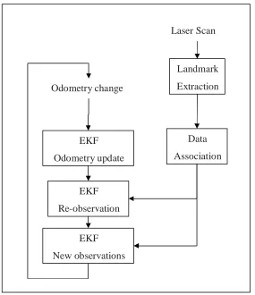
An outline of the SLAM process is given below.

Landmark

Extraction

Data

Association

EKF

Re-observation

EKF

Odometry update

EKF

New observations

Laser Scan

When the odometry changes because the robot moves the uncertainty pertaining to the

robots new position is updated in the EKF using Odometry update. Landmarks are

then extracted from the environment from the robots new position. The robot then

attempts to associate these landmarks to observations of landmarks it previously has

seen. Re-observed landmarks are then used to update the robots position in the EKF.

Landmarks which have not previously been seen are added to the EKF as new

observations so they can be re-observed later. All these steps will be explained in the

next chapters in a very practical fashion relative to how our ER1 robot was

implemented. It should be noted that at any point in these steps the EKF will have an

estimate of the robots current position.

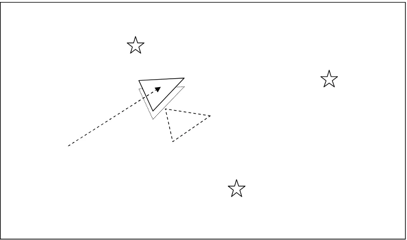
The diagrams below will try to explain this process in more detail:

Figure 3 The robot moves so it now thinks it is here. The distance moved is given by the robots odometry.

Figure 5 As the robot believes more its sensors than its odometry it now uses the information gained about where the landmarks actually are to determine where it is (the location the robot originally thought it was at is illustrated by the dashed triangle).

6.

Laser Data

The first step in the SLAM process is to obtain data about the surroundings of the

robot. As we have chosen to use a laser scanner we get laser data. The SICK laser

scanner we are using can output range measurements from an angle of 100° or 180°.

It has a vertical resolution of 0.25°, 0.5° or 1.0°, meaning that the width of the area

the laser beams measure is 0.25°, 0.5° or 1.0° wide. A typical laser scanner output

will look like this:

2.98, 2.99, 3.00, 3.01, 3.00, 3.49, 3.50, ...., 2.20, 8.17, 2.21

The output from the laser scanner tells the ranges from right to left in terms of meters.

If the laser scanner for some reason cannot tell the exact length for a specific angle it

will return a high value, we are using 8.1 as the threshold to tell if the value is an

error. Some laser scanners can be configured to have ranges longer than 8.1 meters.

Lastly it should be noted that laser scanners are very fast. Using a serial port they can

be queried at around 11 Hz.

The code to interface with the laser scanner can be seen in Appendix B: SICK LMS

7.

Odometry Data

An important aspect of SLAM is the odometry data. The goal of the odometry data is

to provide an approximate position of the robot as measured by the movement of the

wheels of the robot, to serve as the initial guess of where the robot might be in the

EKF. Obtaining odometry data from an ER1 robot is quite easy using the built-in

telnet server. One can just send a text string to the telnet server on a specific port and

the server will return the answer.

The difficult part about the odometry data and the laser data is to get the timing

right. The laser data at some time t will be outdated if the odometry data is retrieved

later. To make sure they are valid at the same time one can extrapolate the data. It is

easiest to extrapolate the odometry data since the controls are known. It can be really

hard to predict how the laser scanner measurements will be. If one has control of

when the measurements are returned it is easiest to ask for both the laser scanner

values and the odometry data at the same time. The code to interface with the ER1

8.

Landmarks

Landmarks are features which can easily be re-observed and distinguished from the

environment. These are used by the robot to find out where it is (to localize itself).

One way to imagine how this works for the robot is to picture yourself blindfolded. If

you move around blindfolded in a house you may reach out and touch objects or hug

walls so that you don’t get lost. Characteristic things such as that felt by touching a

doorframe may help you in establishing an estimate of where you are. Sonars and

laser scanners are a robots feeling of touch.

Below are examples of good landmarks from different environments:

Figure 8 The wooden pillars at a dock may be good landmarks for an underwater vehicle.

As you can see the type of landmarks a robot uses will often depend on the

environment in which the robot is operating.

Landmarks should be re-observable by allowing them for example to be viewed

(detected) from different positions and thus from different angles.

Landmarks should be unique enough so that they can be easily identified from one

time-step to another without mixing them up. In other words if you re-observe two

landmarks at a later point in time it should be easy to determine which of the

landmarks is which of the landmarks we have previously seen. If two landmarks are

very close to each other this may be hard.

Landmarks you decide a robot should recognize should not be so few in the

environment that the robot may have to spend extended time without enough visible

landmarks as the robot may then get lost.

If you decide on something being a landmark it should be stationary. Using a person

as a landmark is as such a bad idea. The reason for this criterion is fairly

straightforward. If the landmark is not always in the same place how can the robot

know given this landmark in which place it is.

9.

Landmark Extraction

Once we have decided on what landmarks a robot should utilize we need to be able to

somehow reliable extract them from the robots sensory inputs.

As mentioned in the introduction there are multiple ways to do landmark extraction

and it depends largely on what types of landmarks are attempted extracted as well as

what sensors are used.

We will present basic landmark extraction algorithms using a laser scanner. They will

use two landmark extraction algorithm called Spikes and RANSAC.

Spike landmarks

The spike landmark extraction uses extrema to find landmarks. They are identified

by finding values in the range of a laser scan where two values differ by more than a

certain amount, e.g. 0.5 meters. This will find big changes in the laser scan from e.g.

when some of the laser scanner beams reflect from a wall and some of the laser

scanner beams do not hit this wall, but are reflected from some things further behind

the wall.

This method is better for finding spikes as it will find actual spikes and not just

permanent changes in range.

Spike landmarks rely on the landscape changing a lot between two laser beams. This

means that the algorithm will fail in smooth environments.

RANSAC

RANSAC (Random Sampling Consensus) is a method which can be used to extract

lines from a laser scan. These lines can in turn be used as landmarks. In indoor

environments straight lines are often observed by laser scans as these are

characteristic of straight walls which usually are common.

RANSAC finds these line landmarks by randomly taking a sample of the laser

readings and then using a least squares approximation to find the best fit line that runs

through these readings. Once this is done RANSAC checks how many laser readings

lie close to this best fit line. If the number is above some threshold we can safely

assume that we have seen a line (and thus seen a wall segment). This threshold is

called the consensus.

The below algorithm outlines the line landmark extraction process for a laser scanner

with a 180° field of view and one range measurement per degree. The algorithm

assumes that the laser data readings are converted to a Cartesian coordinate system –

see Appendix A. Initially all laser readings are assumed to be unassociated to any

lines. In the algorithm we only sample laser data readings from unassociated

readings.

While

• there are still unassociated laser readings,

• and the number of readings is larger than the consensus,

• and we have done less than N trials. do

- Randomly sample S data readings within D degrees of this laser data reading (for example, choose 5 sample readings that lie within 10 degrees of the randomly selected laser data reading).

- Using these S samples and the original reading calculate a least squares best fit line.

- Determine how many laser data readings lie within X centimeters of this best fit line.

- If the number of laser data readings on the line is above some consensus C do the following:

o calculate new least squares best fit line based on all the laser readings determined to lie on the old best fit line.

o Add this best fit line to the lines we have extracted. o Remove the number of readings lying on the line from the

total set of unassociated readings. od

This algorithm can thus be tuned based on the following parameters:

N – Max number of times to attempt to find lines.

S – Number of samples to compute initial line.

D – Degrees from initial reading to sample from.

X – Max distance a reading may be from line to get associated to line.

C – Number of points that must lie on a line for it to be taken as a line.

The EKF implementation assumes that landmarks come in as a range and bearing

from the robots position. One can easily translate a line into a fixed point by taking

another fixed point in the world coordinates and calculating the point on the line

closest to this fixed point. Using the robots position and the position of this fixed

Figure 11 Illustration of how to get an extracted line landmark as a point.

(0,0)

Extracted

point

landmark

Extracted line

landmark

Line

orthogonal to

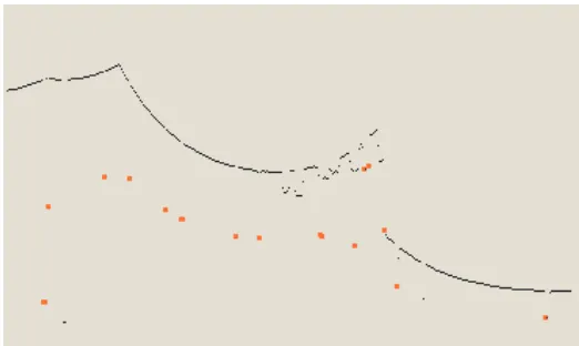
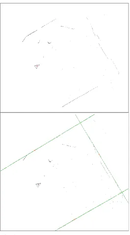
Figure 12 The RANSAC algorithm finds the main lines in a laser scan. The green lines are the best fit lines representing the landmarks. The red dots represent the landmarks approximated to

points. By changing the RANSAC parameters you could also extract the small wall segments. They are not considered very reliable landmarks so were not used. Lastly just above the robot is

a person. RANSAC is robust against people in the laser scan.

Multiple strategies

We have presented two different approaches to landmark extraction. Both extract

different types of landmarks and are suitable for indoor environments. Spikes

however is fairly simple and is not robust against environments with people. The

reason for this is that Spikes picks up people as spikes as they theoretically are good

landmarks (they stand out from the environment).

As RANSAC uses line extraction it will not pick up people as landmarks as they do

not individually have the characteristic shape of a line.

A third method which we will not explore is called scan-matching where you attempt

match two successive laser scans. We name it here for people interested in other

approaches.

Code for landmark extraction algorithms can be found in Appendix D: Landmark

10. Data Association

The problem of data association is that of matching observed landmarks from

different (laser) scans with each other. We have also referred to this as re-observing

landmarks.

To illustrate what is meant by this we will give an example:

For us humans we may consider a chair a landmark. Let us say we are in a room and

see a specific chair. Now we leave the room and then at some later point

subsequently return to the room. If we then see a chair in the room and say that it is

the same chair we previously saw then we have associated this chair to the old chair.

This may seem simple but data association is hard to do well. Say the room had two

chairs that looked practically identical. When we subsequently return to the room we

might not be able to distinguish accurately which of the chairs were which of the

chairs we originally saw (as they all look the same). Our best bet is to say that the

one to the left must be the one we previously saw to the left, and the one to the right

must be the one we previously saw on the right.

In practice the following problems can arise in data association:

-

You might not re-observe landmarks every time step.

-

You might observe something as being a landmark but fail to ever see it again.

-

You might wrongly associate a landmark to a previously seen landmark.

As stated in the landmarks chapter it should be easy to re-observe landmarks. As such

the first two cases above are not acceptable for a landmark. In other words they are

bad landmarks. Even if you have a very good landmark extraction algorithm you may

run into these so it is best to define a suitable data-association policy to minimize this.

We will now define a data-association policy that deals with these issues. We assume

that a database is set up to store landmarks we have previously seen. The database is

usually initially empty. The first rule we set up is that we don’t actually consider a

landmark worthwhile to be used in SLAM unless we have seen it N times. This

eliminates the cases where we extract a bad landmark. The below-mentioned

validation gate is explained further down in the text.

1. When you get a new laser scan use landmark extraction to extract all visible landmarks.

2. Associate each extracted landmark to the closest landmark we have seen more than N times in the database.

3. Pass each of these pairs of associations (extracted landmark, landmark in database) through a validation gate.

a. If the pair passes the validation gate it must be the same landmark we have re-observed so increment the number of times we have seen it in the database.

b. If the pair fails the validation gate add this landmark as a new landmark in the database and set the number of times we have seen it to 1.

This technique is called the nearest-neighbor approach as you associate a landmark

with the nearest landmark in the database.

The simplest way to calculate the nearest landmark is to calculate the Euclidean

distance.

Other methods include calculating the Mahalanobis distance which is

better but more complicated. This was not used in our approach as RANSAC

landmarks usually are far apart which makes using the Euclidean distance suitable.

The validation gate uses the fact that our EKF implementation gives a bound on the

uncertainty of an observation of a landmark. Thus we can determine if an observed

landmark is a landmark in the database by checking if the landmark lies within the

area of uncertainty. This area can actually be drawn graphically and is known as an

error ellipse.

By setting a constant

λ

an observed landmark is associated to a landmark if the

Where vi is the innovation and Si is the innovation covariance defined in the EKF

11. The EKF

The Extended Kalman Filter is used to estimate the state (position) of the robot from

odometry data and landmark observations. The EKF is usually described in terms of

state estimation alone (the robot is given a perfect map). That is, it does not have the

map update which is needed when using EKF for SLAM. In SLAM vs. a state

estimation EKF especially the matrices are changed and can be hard to figure out how

to implement, since it is almost never mentioned anywhere. We will go through each

of these. Most of the EKF is standard, as a normal EKF, once the matrices are set up,

it is basically just a set of equations.

Overview of the process

As soon as the landmark extraction and the data association is in place the SLAM

process can be considered as three steps:

1.

Update the current state estimate using the odometry data

2.

Update the estimated state from re-observing landmarks.

3.

Add new landmarks to the current state.

The first step is very easy. It is just an addition of the controls of the robot to the old

state estimate. E.g. the robot is at point (x, y) with rotation theta and the controls are

(dx, dy) and change in rotation is dtheta. The result of the first step is the new state of

the robot (x+dx, y+dy) with rotation theta+dtheta.

In the second step the re-observed landmarks are considered. Using the estimate of the

current position it is possible to estimate where the landmark should be. There is

usually some difference, this is called the innovation. So the innovation is basically

the difference between the estimated robot position and the actual robot position,

the uncertainty of the current landmark position is very little. Re-observing a

landmark from this position with low uncertainty will increase the landmark certainty,

i.e. the variance of the landmark with respect to the current position of the robot.

In the third step new landmarks are added to the state, the robot map of the world.

This is done using information about the current position and adding information

about the relation between the new landmark and the old landmarks.

The matrices

It should be noted that there is a lot of different notions for the same variables in the

different papers. We use some fairly common notions.

The system state: X

X is probably one of the most important matrices in the system along with the

covariance matrix. It contains the position of the robot, x, y and theta.

Furthermore it contains the x and y position of each landmark. The matrix can

be seen to the right. It is important to have the matrix as a vertical matrix to

make sure that all the equations will work. The size of X is 1 column wide

and 3+2*n rows high, where n is the number of landmarks. Usually the values

saved will be in either meters or millimeters for the ranges. Which one is used does

not matter, it is just important, of course, to use the same notion everywhere. The

bearing is saved in either degrees or radians. Again it is a question of using the same

notion everywhere.

xr

yr

thetar

The covariance matrix: P

Quick math recap:

The covariance of two variates provides a measure of how strongly correlated these

two variables are. Correlation is a concept used to measure the degree of linear

dependence between variables.

The covariance matrix P is a very central matrix in the system. It contains the

covariance on the robot position, the covariance on the landmarks, the covariance

between robot position and landmarks and

finally it contains the covariance between

the landmarks. The figure on the right

shows the content of the covariance

matrix P. The first cell, A contains the

covariance on the robot position. It is a 3

by 3 matrix (x, y and theta). B is the

covariance on the first landmark. It is a 2 by 2 matrix, since the landmark does not

have an orientation, theta. This continues down to C, which is the covariance for the

last landmark. The cell D contains the covariance between the robot state and the first

landmark. The cell E contains the covariance between the first landmark and the robot

state. E can be deduced from D by transposing the sub-matrix D. F contains the

covariance between the last landmark and the first landmark, while G contains the

covariance between the first landmark and the last landmark, which again can be

deduced by transposing F. So even though the covariance matrix may seem

complicated it is actually built up very systematically. Initially as the robot has not

seen any landmarks the covariance matrix P only includes the matrix A. The

covariance matrix must be initialized using some default values for the diagonal. This

reflects uncertainty in the initial position. Depending on the actual implementation

there will often be a singular error if the initial uncertainty is not included in some of

the calculations, so it is a good idea to include some initial error even though there is

reason to believe that the initial robot position is exact.

... ...

... ...

A

E

... ...

... ...

D

B

... ...

G

...

...

...

... ... ... ... ... ...

...

...

...

... ... ... ... ... ...

... ...

F

The Kalman gain: K

The Kalman gain K is computed to find out how much we will trust the observed

landmarks and as such how much we want to gain from the new knowledge they

provide. If we can see that the robot should be moved 10 cm to the right, according to

the landmarks we use the Kalman Gain to find out how much we actually correct the

position, this may only be 5 cm because we do not trust the landmarks

completely, but rather find a compromise between the odometry and the

landmark correction. This is done using the uncertainty of the observed

landmarks along with a measure of the quality of the range measurement

device and the odometry performance of the robot. If the range

measurement device is really bad compared to the odometry performance

of the robot, we of course do not trust it very much, so the Kalman gain

will be low. On the contrary, if the range measurement device is very good compared

to the odometry performance of the robot the Kalman gain will be high. The matrix

can be seen to the right. The first row shows how much should be gained from the

innovation for the first row of the state X. The first column in the first row describes

how much should be gained from the innovation in terms of range, the second column

in the first row describes how much should be gained from the innovation in terms of

the bearing. Again both are for the first row in the state, which is the x value of the

robot position. The matrix continues like down through the robot position; the first

three rows, and the landmarks; each two new rows. The size of the matrix is 2

columns and 3+2*n rows, where n is the number of landmarks.

The Jacobian of the measurement model: H

The Jacobian of the measurement model is closely related to the measurement model,

of course, so let’s go through the measurement model first. The measurement model

defines how to compute an expected range and bearing of the measurements

(observed landmark positions). It is done using the following formula, which is

denoted h:

Where lambda x is the x position of the landmark, x is the current estimated robot x

position, lambda y is the y position of the landmark and y is the current estimated

robot y position. Theta is the robot rotation. This will give us the predicted

measurement of the range and bearing to the landmark. The Jacobian of this matrix

with respect to x, y and theta, H, is:

H shows us how much the range and bearing changes as x, y and theta changes. The

first element in the first row is the change in range with respect to the change in the x

axis. The second element is with respect to the change in the y axis. The last element

is with respect to the change in theta, the robot rotation. Of course this value is zero as

the range does not change as the robot rotates. The second row gives the same

information, except that this is the change in bearing for the landmark. This is the

contents of the usual H for regular EKF state estimation. When doing SLAM we need

some additional values for the landmarks:

When using the matrix H e.g. for landmark number two we will be using the matrix

above. The upper row is for information purposes only; it is not part of the matrix.

Xr

Yr

Tr

X1

Y1

X2

Y2

X3

Y3

A

B

C

0

0

-A

-B

0

0

This means that the first 3 columns are the regular H, as for regular EKF state

estimation. For each landmark we add two columns. When using the H matrix for

landmark two as above we fill it out like above with X2 set to –A and –D and Y2 set

to –B and -E. The columns for the rest of the landmarks are 0. are the same as the first

two columns of the original H, just negated. We only use two terms, X2 and Y2,

because the landmarks do not have any rotation.

The Jacobian of the prediction model: A

Like H, the Jacobian of the prediction model is closely related to the prediction

model, of course, so let’s go through the prediction model first. The prediction model

defines how to compute an expected position of the robot given the old position and

the control input. It is done using the following formula, which is denoted f:

f =

Where x and y is the robot position, theta the robot rotation, t is the change in thrust

and q is the error term. We are using the change in position directly from the

odometry input from the ER1 system, so we use x, y, theta and x, y and theta

directly and the process noise, described later:

x + x + x * q

y + y + y * q

theta + theta + theta * q

The calculations are the same as for the H matrix, except that we now have one more

row for the robot rotation. Since it is only used for robot position prediction it will

also not be extended for the rest of the landmarks. As can be seen from the first

matrix, the prediction model, the term – t * sin theta is the same as - y in our case

and – t * cos theta is the same as x. So we can just use our control terms, yielding:

1

0

- y

0

1

x

0

0

1

The SLAM specific Jacobians: J

and J

When doing SLAM there are some Jacobians which are only used in SLAM. This is

of course in the integration of new features, which is the only step that differs from

regular state estimation using EKF. The first is Jxr. It is basically the same as the

jacobian of the prediction model, except that we start out without the rotation term. It

is the jacobian of the prediction of the landmarks, which does not include prediction

of theta, with respect to the robot state [x, y, theta] from X:

J

=

The jacobian Jz is also the jacobian of the prediction model for the landmarks, but this

time with respect to [range, bearing]. This in turn yields:

J

=

The process noise: Q and W

The process is assumed to have a gaussian.noise proportional to the controls, x, y

and t. The noise is denoted Q, which is a 3 by 3 matrix. It

is usually calculated by multiplying some gaussian sample

C with W and W transposed:

Q = WCW

C is be a representation of how exact the odometry is. The value should be set

according to the robot odometry performance and is usually easiest to set by

experiments and tuning the value.

In most papers the process noise is either denoted Q alone or as WQW

. The notion C

is basically never used, but is needed here to show the two approaches.

The measurement noise: R and V

The range measurement device is also assumed to have gaussian noise proportional to

the range and bearing. It is calculated as VRV

. V is just a 2 by 2 identity matrix. R is

also a 2 by 2 matrix with numbers only in the diagonal. In the upper left

corner we have the range, r, multiplied by some constants c and d. The

constants should represent the accuracy of the measurement device. If for example the

range error has 1 cm variance it should, c should be a gaussian with variance 0.01. If

the bearing error is always 1 degree bd should be replaced with the number 1,

presuming that degrees are used for measurements. Usually it will not make sense to

make the error on the angle proportional with the size of the angle.

c x

c y

c t

Step 1: Update current state using the odometry data

This step, called the prediction step we update the current state using the odometry

data. That is we use the controls given to the robot to calculate an estimate of the new

position of the robot. To update the current state we use the following equation:

In our simple odometry model we can simply just add the controls as noted in a

previous chapter:

x + x

y + y

theta + theta

This should be updated in the first three spaces in the state vector, X. We also need to

update the A matrix, the jacobian of the prediction model, every iteration:

1

0

- y

0

1

x

0

0

1

Also Q should be updated to reflect the control terms, x, y and t:

Finally we can calculate the new covariance for the robot position. Since the

covariance for the robot position is just the top left 3 by 3 matrix of P we will only

update this:

P

= A P

A + Q

Where the symbol P

is the top left 3 by 3 matrix of P.

c x

c x y c x t

cc y x c y

c y t

Now we have updated the robot position estimate and the covariance for this position

estimate. We also need to update the robot to feature cross correlations. This is the top

3 rows of the covariance matrix:

P

= A P

Step 2: Update state from re-observed landmarks

The estimate we obtained for the robot position is not completely exact due to the

odometry errors from the robot. We want to compensate for these errors. This is done

using landmarks. The landmarks have already been discussed including how to

observe them and how to associate them to already known landmarks. Using the

associated landmarks we can now calculate the displacement of the robot compared to

what we think the robot position is. Using the displacement we can update the robot

position. This is what we want to do in step 2. This step is run for each re-observed

landmark. Landmarks that are new are not dealt with until step 3. Delaying the

incorporation of new landmarks until the next step will decrease the computation cost

needed for this step, since the covariance matrix, P, and the system state, X, are

smaller.

We will try to predict where the landmark is using the current estimated robot position

(x, y) and the saved landmark position (

λ

x,

λ

y). With the following formula:

We get the range and bearing to the landmark, h, also seen when calculating the

jacobian H. This can be compared to the range and bearing for the landmark we get

As previously stated the values are calculated as follows:

Again, remember that only the first three columns and the columns valid for the

current landmark should be filled out.

The error matrix R should also be updated to reflect the range and bearing in the

current measurements. A good starting value for rc is the range value

multiplied with 0.01, meaning there is 1 % error in the range. A good error

for the bd value is 1, meaning there is 1 degree error in the measurements. This error

should not be proportional with the size of the angle; this would not make sense, of

course.

Now we can compute the Kalman gain. It is calculated using the following formula:

K = P * H

* (H * P * H

+ V * R * V

)

The Kalman now contains a set of numbers indicating how much each of the

landmark positions and the robot position should be updated according to the

re-observed landmark. The term (H * P * H

+ V * R * V

) is called the innovation

covariance, S, it is also used in the Data Association chapter when calculating the

validation gate for the landmark.

Finally we can compute a new state vector using the Kalman gain:

Xr

Yr

Tr

X1

Y1

X2

Y2

X3

Y3

A

B

C

0

0

-A

-B

0

0

D

E

F

0

0

-D

-E

0

0

X = X + K * (z – h)

This operation will update the robot position along with all the landmark positions,

given the term (z-h) does not result in (0, 0). Note that (z-h) yields a result of two

numbers which is the displacement in range and bearing, denoted v.

This process is repeated for each matched landmark.

Step 3: Add new landmarks to the current state

In this step we want to update the state vector X and the covariance matrix P with new

landmarks. The purpose is to have more landmarks that can be matched, so the robot

has more landmarks that can be matched.

First we add the new landmark to the state vector X

X = [X xN yN]

Also we need to add a new row and column to the covariance matrix, shown in the

figure below as the grey area. First we add the covariance for the new landmark in the

cell C, also called P

, since it is the

covariance for the N+1 landmark:

P

= Jxr P Jxr

+ JzRJz

After this we add the robot – landmark

covariance for the new landmark. This

corresponds to the upper left corner of the

covariance matrix. It is computed as follows:

P

= P

J

... ...

... ...

A

E

... ...

... ...

D

B

... ...

G

...

...

...

... ... ... ... ... ...

...

...

...

... ... ... ... ... ...

... ...

F

Finally the landmark – landmark covariance needs to be added (the lowest row):

P

= Jxr (P

)

Again the landmark – landmark covariance on the other side of the diagonal matrix is

the transposed value:

P

= (P

)

This completes the last step of the SLAM process. The robot is now ready to move

again, observe landmarks, associate landmarks, update the system state using

odometry, update the system state using re-observed landmarks and finally add new

12. Final remarks

The SLAM presented here is a very basic SLAM. There is much room for

improvement, and there are areas that have not even been touched. For example there

is the problem of closing the loop. This problem is concerned with the robot returning

to a place it has seen before. The robot should recognize this and use the new found

information to update the position. Furthermore the robot should update the

landmarks found before the robot returned to a known place, propagating the

correction back along the path. A system such as ATLAS [2] is concerned with this.

It is also possible to combine this SLAM with an occupation grid, mapping the world

in a human-readable format. Besides the obvious use for an occupation grid as a

human-readable map, occupation grids can also be used for path planning. A* and D*

13. References:

1. Koenig, Likhachev: Incremental A* (D*)

2. Bosse, Newman, Leonard, Soika, Feiten, Teller: An ATLAS framework

3. Roy: Foundations of state estimation (lecture):

4. Zunino: SLAM in realistic environments:

http://www.nada.kth.se/utbildning/forsk.utb/avhandlingar/lic/020220.pdf

5. Welch, Bishop: An introduction to the Kalman Filter:

6. Smith, Self, Cheesman: Estimating uncertain spatial relationships in robotics 7. Leonard, Durrant-Whyte: Mobile robot localization by tracking geometric beacons:

8. Se, Lowe, Little: Mobile Robot Localization and Mapping using Scale-Invariant Visual Landmarks:

http://www.cs.ubc.ca/~se/papers/ijrr02.pdf

9. SICK, industrial sensors:

http://www.sick.de

10. Evolution Robotics

14. Appendix A: Coordinate conversion

Conversion from range and bearing to Cartesian coordinates:

)

(

*

Cos

range

x

=

θ

)

(

*

Sin

range

y

=

−

θ

Converts an observation from the robots sensors to Cartesian coordinates. Where

θ

is the angle the observation is viewed at and range is the distance to the measurement.

To get the coordinates with respect to a world map you must also add the robots angle

r

θ

relative to the world map:

)

(

*

Cos

range

x

=

θ +

θ

)

(

*

Sin

range

15. Appendix B: SICK LMS 200 interface code

LMS Interface code:

using System;

using SerialPorts;

namespace APULMS

{

/// <summary>

/// Summary description for LMS200.

/// </summary>

public class LMS200

{

private Threader th;

public SerialPort Port;

private WithEvents Func;

private int PortIndex;

private static byte[] GET_MEASUREMENTS = {0x02, 0x00, 0x02, 0x00, 0x30, 0x01, 0x31, 0x18};

private static byte[] PCLMS_B9600 = {0x02,0x00,0x02,0x00,0x20,0x42,0x52,0x08};

private static byte[] PCLMS_B19200 = {0x02,0x00,0x02,0x00,0x20,0x41,0x51,0x08};

private static byte[] PCLMS_B38400 = {0x02,0x00,0x02,0x00,0x20,0x40,0x50,0x08};

public LMS200(Threader t, int PortIndex)

{

this.th = t;

this.PortIndex = PortIndex;

// Instantiate base class event handlers.

this.Func = new WithEvents();

this.Func.Error = new StrnFunc(this.OnError);

this.Func.RxChar = new ByteFunc(this.OnRecvI);

this.Func.CtsSig = new BoolFunc(this.OnCts);

this.Func.DsrSig = new BoolFunc(this.OnDsr);

this.Func.RingSig = new BoolFunc(this.OnRing);

// Instantiate the terminal port.

this.Port = new SerialPort(this.Func);

this.Port.Cnfg.BaudRate = SerialPorts.LineSpeed.Baud_9600;

this.Port.Cnfg.Parity = SerialPorts.Parity.None;

PortControl(); }

/// <summary>

/// Gives one round of measurements

/// </summary>

public void getMeasurements()

{

SendBuf(GET_MEASUREMENTS); }

public void setBaud(bool fast)

{

if (fast) {

SendBuf(PCLMS_B38400);

Port.Cnfg.BaudRate = SerialPorts.LineSpeed.Baud_38400; }

else

{

SendBuf(PCLMS_B19200);

Port.Cnfg.BaudRate = SerialPorts.LineSpeed.Baud_19200; }

}

public void ClosePorts()

{

{

if(this.Port.IsOpen == false) {

if(this.Port.Open(PortIndex) == false) { // ERROR return; } else { // OK } } else {

if(this.Port.IsOpen) {

this.Port.Close(); }

// OK

this.Port.Signals(); }

return;

}

/// <summary>

/// Handles error events.

/// </summary>

internal void OnError(string fault)

{

//this.Status.Text = fault; PortControl();

}

/// <summary>

/// </summary>

internal void OnRecvI(byte[] b)

{ }

/// <summary>

/// Set the modem state displays.

/// </summary>

internal void OnCts(bool cts)

{

System.Threading.Thread.Sleep(1); }

/// <summary>

/// Set the modem state displays.

/// </summary>

internal void OnDsr(bool dsr)

{

System.Threading.Thread.Sleep(1); Color.Red;

}

/// <summary>

/// Set the modem state displays.

/// </summary>

internal void OnRlsd(bool rlsd)

{

System.Threading.Thread.Sleep(1); }

/// <summary>

/// Set the modem state displays.

/// </summary>

}

/// <summary>

/// Transmit a buffer.

/// </summary>

private uint SendBuf(byte[] b)

{

uint nSent=0;

if(b.Length > 0) {

nSent = this.Port.Send(b);

if(nSent != b.Length) {

// ERROR }

}

return nSent;

}

Thread for retrieving the data:

using System;

using SerialPorts;

using System.Threading;

namespace APULMS

{

/// <summary>

/// Summary description for Threader.

/// </summary>

public class Threader

{

public byte[] buffer;

public int bufferSize;

public int bufferWritePointer;

public int bufferReadPointer;

public SerialPort p;

public bool cont = true;

public Threader(int BufferSize)

{

this.bufferSize = BufferSize;

buffer = new byte[this.bufferSize]; ResetBuffer();

}

public Threader()

{

this.bufferSize = 20000;

buffer = new byte[this.bufferSize]; ResetBuffer();

bufferWritePointer = 0; bufferReadPointer = 0;

for (int i = 0; i < this.bufferSize; i++) buffer[i] = 0x00;

}

private int pwrap(int p)

{

while (p >= bufferSize)

p -= bufferSize;

return (p);

}

public void getData()

{

byte[] b;

uint nBytes;

int count = 0;

while (true)

{

// Get number of bytes nBytes = this.p.Recv(out b);

if(nBytes > 0) {

int i = 0;

for (; i < nBytes && i < b.Length; i++)

buffer[pwrap(bufferWritePointer+i)] = b[i]; bufferWritePointer = pwrap(bufferWritePointer + i); // restart no data counter

count = 0; }

else

{

// no data, count up count++;

if (count > 100) {

// Wait until told to resume Monitor.Wait(this);

// Reset counter after wait count = 0;

} }

} }

16. Appendix C: ER1 interface code

ER1 interface code, ApplicationSettings.cs:

//--- // <autogenerated>

// This code was generated_u98 ?y a tool. // Runtime Version: 1.0.3705.0

//

// Changes to this file may cause incorrect behavior and will be lost if // the code is regenerated.

// </autogenerated>

//---

namespace ER1 {

using System;

using System.Data;

using System.Xml;

using System.Runtime.Serialization;

[Serializable()]

[System.ComponentModel.DesignerCategoryAttribute("code")] [System.Diagnostics.DebuggerStepThrough()]

[System.ComponentModel.ToolboxItem(true)]

public class ApplicationSettings : DataSet_u123 ?

private ER1DataTable tableER1;

public ApplicationSettings()_u123 ? this.InitClass();

System.ComponentModel.CollectionChangeEventHandler schemaChangedHandler = new

}

protected ApplicationSettings(SerializationInfo info, StreamingContext context) { string strSchema = ((string)(info.GetValue("XmlSchema", typeof(string)))); if ((strSchema != null)) {

DataSet ds = new DataSet();

ds.ReadXmlSchema(new XmlTextReader(new System.IO.StringReader(strSchema))); if ((ds.Tables["ER1"] != null)) {

this.Tables.Add(new ER1DataTable(ds.Tables["ER1"])); }

this.DataSetName = ds.DataSetName; this.Prefix = ds.Prefix;

this.Namespace = ds.Namespace; this.Locale = ds.Locale;

this.CaseSensitive = ds.CaseSensitive;

this.EnforceConstraints = ds.EnforceConstraints;

this.Merge(ds, false, System.Data.MissingSchemaAction.Add); this.InitVars();

} else {

this.InitClass(); }

this.GetSerializationData(info, context);

System.ComponentModel.CollectionChangeEventHandler schemaChangedHandler = new

System.ComponentModel.CollectionChangeEventHandler(this.SchemaChanged); this.Tables.CollectionChanged += schemaChangedHandler; this.Relations.CollectionChanged += schemaChangedHandler; }

[System.ComponentModel.Browsable(false)]

[System.ComponentModel.DesignerSerializationVisibilityAttribute(System.ComponentModel.DesignerSerializationVisibilit y.Content)]

} }

public override DataSet Clone() {

ApplicationSettings cln = ((ApplicationSettings)(base.Clone())); cln.InitVars();

return cln; }

protected override bool ShouldSerializeTables() { return false;

}

protected override bool ShouldSerializeRelations() { return false;

}

protected override void ReadXmlSerializable(XmlReader reader) { this.Reset();

DataSet ds = new DataSet(); ds.ReadXml(reader);

if ((ds.Tables["ER1"] != null)) {

this.Tables.Add(new ER1DataTable(ds.Tables["ER1"])); }

this.DataSetName = ds.DataSetName; this.Prefix = ds.Prefix;

this.Namespace = ds.Namespace; this.Locale = ds.Locale;

this.CaseSensitive = ds.CaseSensitive;

this.EnforceConstraints = ds.EnforceConstraints;

this.Merge(ds, false, System.Data.MissingSchemaAction.Add); this.InitVars();

}

this.WriteXmlSchema(new XmlTextWriter(stream, null)); stream.Position = 0;

return System.Xml.Schema.XmlSchema.Read(new XmlTextReader(stream), null); }

internal void InitVars() {

this.tableER1 = ((ER1DataTable)(this.Tables["ER1"])); if ((this.tableER1 != null)) {

this.tableER1.InitVars(); }

}

private void InitClass() {

this.DataSetName = "ApplicationSettings"; this.Prefix = "";

this.Namespace = "http://tempuri.org/ApplicationSettings.xsd"; this.Locale = new System.Globalization.CultureInfo("en-US"); this.CaseSensitive = false;

this.EnforceConstraints = true; this.tableER1 = new ER1DataTable(); this.Tables.Add(this.tableER1); }

private bool ShouldSerializeER1() { return false;

}

private void SchemaChanged(object sender, System.ComponentModel.CollectionChangeEventArgs e) { if ((e.Action == System.ComponentModel.CollectionChangeAction.Remove)) {

this.InitVars(); }

}

public class ER1DataTable : DataTable, System.Collections.IEnumerable {

private DataColumn columnIP;

private DataColumn columnPassword;

private DataColumn columnPort;

internal ER1DataTable() : base("ER1") { this.InitClass(); }

internal ER1DataTable(DataTable table) : base(table.TableName) {

if ((table.CaseSensitive != table.DataSet.CaseSensitive)) { this.CaseSensitive = table.CaseSensitive;

}

if ((table.Locale.ToString() != table.DataSet.Locale.ToString())) { this.Locale = table.Locale;

}

if ((table.Namespace != table.DataSet.Namespace)) { this.Namespace = table.Namespace;

}

this.Prefix = table.Prefix;

this.MinimumCapacity = table.MinimumCapacity; this.DisplayExpression = table.DisplayExpression; }

[System.ComponentModel.Browsable(false)] public int Count {

get {

return this.Rows.Count; }

internal DataColumn IPColumn { get {

return this.columnIP; }

}

internal DataColumn PasswordColumn { get {

return this.columnPassword; }

}

internal DataColumn PortColumn { get {

return this.columnPort; }

}

public ER1Row this[int index] { get {

return ((ER1Row)(this.Rows[index])); }

}

public event ER1RowChangeEventHandler ER1RowChanged;

public event ER1RowChangeEventHandler ER1RowChanging;

public event ER1RowChangeEventHandler ER1RowDeleted;

public event ER1RowChangeEventHandler ER1RowDeleting;

public ER1Row AddER1Row(string IP, string Password, int Port) { ER1Row rowER1Row = ((ER1Row)(this.NewRow()));

rowER1Row.ItemArray = new object[] { IP,

Password, Port};

this.Rows.Add(rowER1Row); return rowER1Row;

}

public System.Collections.IEnumerator GetEnumerator() { return this.Rows.GetEnumerator();

}

public override DataTable Clone() {

ER1DataTable cln = ((ER1DataTable)(base.Clone())); cln.InitVars();

return cln; }

protected override DataTable CreateInstance() { return new ER1DataTable();

}

internal void InitVars() {

this.columnIP = this.Columns["IP"];

this.columnPassword = this.Columns["Password"]; this.columnPort = this.Columns["Port"];

}

private void InitClass() {

this.columnIP = new DataColumn("IP", typeof(string), null, System.Data.MappingType.Element); this.Columns.Add(this.columnIP);

this.columnPassword = new DataColumn("Password", typeof(string), null, System.Data.MappingType.Element);

this.columnPort = new DataColumn("Port", typeof(int), null, System.Data.MappingType.Element); this.Columns.Add(this.columnPort);

}

public ER1Row NewER1Row() {

return ((ER1Row)(this.NewRow())); }

protected override DataRow NewRowFromBuilder(DataRowBuilder builder) { return new ER1Row(builder);

}

protected override System.Type GetRowType() { return typeof(ER1Row);

}

protected override void OnRowChanged(DataRowChangeEventArgs e) { base.OnRowChanged(e);

if ((this.ER1RowChanged != null)) {

this.ER1RowChanged(this, new ER1RowChangeEvent(((ER1Row)(e.Row)), e.Action)); }

}

protected override void OnRowChanging(DataRowChangeEventArgs e) { base.OnRowChanging(e);

if ((this.ER1RowChanging != null)) {

this.ER1RowChanging(this, new ER1RowChangeEvent(((ER1Row)(e.Row)), e.Action)); }

}

protected override void OnRowDeleted(DataRowChangeEventArgs e) { base.OnRowDeleted(e);

if ((this.ER1RowDeleted != null)) {