Issues
ISSN: 2146-4138
available at http: www.econjournals.com
International Journal of Economics and Financial Issues, 2016, 6(1), 7-12.
Does Poverty Influence Prevalence of Child Labor in Developing
Countries?
Idris Isyaku Abdullahi
1,2*, Zaleha Mohd Noor
1, Rusmawati Said
1, Ahmad Zubaidi Baharumshah
11Department of Economics, Faculty of Economics and Management, University Putra Malaysia, 43400 Serdang, Selangor, Malaysia, 2Department of Accounting and Finance Technology, Faculty of Management Technology, Abubakar Tafawa Balewa University,
Bauchi, Nigeria. *Email: [email protected]
ABSTRACT
The present article examined the impact of poverty on child labor prevalence across 42 developing countries based on system-generalize method of moment technique. The main result on the linkage between child labor prevalence and poverty deviated from the popular beliefs in majority of the existing literature that poverty caused child labor prevalence. The finding indicated that poverty is negatively related to child labor prevalence, in the sense that the higher the poverty the lower the child labor prevalence in the sample countries investigated, this finding therefore reconfirmed the wealth paradox of Bhalotra and Heady (2003).
Keywords: Poverty, Remittance, Child Labor Prevalence, System-Generalize Method of Moment, Wealth Paradox, Developing Countries JEL Classifications: P46, F24, Z22.
1. INTRODUCTION
The use of children in employment in developing economies constitutes one of the major problems bedeviling the societies. In recent times, there has been an increase in the global focus regarding the menace of child labor. This emanates to various studies conducted by researchers with a view to provide policy recommendations so as to bring the menace to its barest minimal and subsequent elimination. According to International Programme on the Elimination of Child labor, an estimated 168 million children were involved into various economic activities worldwide, which account for approximately 11% of the entire children population
as a whole (IPEC-ILO, 2013). Almost all of them are subjected
to working for a longer period of time in activities that relates to unhealthy environments, mostly shouldering responsibilities, bigger than their individual capabilities, sometimes with meager pay, less food, lack of access to education and above all with less attention medically. It is a common but not disputed perception that children participation in labor activities is propelled by parents. It is however, not clear whether increase in household income helps in eliminating child labor or instrumental factor was the introduction of relevant legislation. This is because increase in
aggregate income may not necessarily lead to an increase in the households’ income who is the suppliers of labor. An empirical
examination of whether child labor is influence by the poverty level
in the developing countries will be provided in the section below.
Figure 1 indicates the selected developing countries during
2009-2013, poverty is positively related to child labor, since an
increase in the rate of poverty results in a corresponding increase in the level of child labor. This is in support of the popular wisdom that poverty leads to an increase in child labor prevalence. However, the result of the study presented below, indicated a direct opposite of the trend that is a negative relationship as supported
by wealth paradox advanced by Bhalotra and Heady (2003).
2. LITERATURE REVIEW
The role poverty plays in influencing the participation of children
in labor activities draw an increasing attention in recent times. An
early empirical support regarding whether poverty is influencing
child labor or not in developing countries were provided by some
luxury axiom in an attempt to highlight the fact that poverty caused child labor. His attention was focused on parent preference in
which case parent value leisure of their children, though; when
they are poor they will not be able to afford it. More concisely, he considered the hypothesis that parents preference towards child leisure is such that they send them to work only when their income is below a subsistence consumption level.
In a similar vein, Blunch and Verner (2001), revisited the link between poverty and child labor in Ghana. The research finding reaffirmed that poverty is positively related to child labor as
against the postulation by the recent literature which question the existence of positive relationship between poverty and child labor.
Furthermore, Nkamleu (2006), postulated that recent researches in the field of economics, questioned the validity of the proposed
link between poverty and child labor which was traditionally established, suggesting that child labor is more noticeable in the
richest households (wealth paradox). His study revisited the link
between poverty and farm child labor in Africa, with the aim
of testing the paradoxical wealth effect. The research findings
indicated a mixed reaction, with the effect of different commonly used wealth proxies showing a negative effect on child labor participation, while the relevant and robust wealth proxies show a positive relationship between poverty and child labor.
Recent studies on poverty and child labor comprises of the work
by Dumas (2007) who explored that, often argued by various
researchers is the fact that the predominant factor leading to child labor is poverty. Though, majority of the children that partake into child laboring dwells from rural areas which are mostly
identified by substantial labor market imperfections. Using a
model of rural households’ labor supply which is developed to provide testable implication for the two contradicting hypotheses
on poverty which includes; that child labor occurs resulting from
subsistence constraint and that children leisure is a luxury good.
The research finding indicated that in rural Burkina Faso children
do not engage in child laboring in order to meet subsistence needs
of their families. Labor market imperfection is identified as the
main factor that motivates children’s engagement in child labor activities in Burkina Faso.
Basu et al. (2010) postulated that it was revealed by some studies
that greater possession of land wealth by households were responsible for higher participation of children in child labor, hence casting doubt on the hypothesis which says child labor is caused by poverty. Their paper developing a simple model which suggested the possibility of an inverted-U-relationship between land possession and child laboring using a data from northern India. It was found that after controlling for child, households and village characteristics, the turning point beyond which possession of more land results in a decrease of child labor happened around 4 acres of land per household. It could be deduced that additional land possession beyond 4 acres enable the families to experience decrease in their child labor participation rate, which means that the families with 1 acre that experience rise in land possession up to 4 acres tend to have increase in their child labor participation rate. This indicated existence of an inverted U relationship between land possession and child labor participation rate, with initial increase in child labor resulting from increase in land possession from 1 acre to 4 acres and a subsequent fall in child labor participation rate resulting from land possession beyond 4 acres of land.
Furthermore, Bhalotra and Heady (2003) conducting a study on
Ghana and Pakistan found that child labor use mostly emerges
from the richest households. The study finding was based on the
observation that children in land rich households are more likely to work and attend school less compared to the children in land poor households. This phenomenon is referred to as wealth paradox. This results from the fact that greater majority of the children that engages in child labor activities in developing countries relates to agricultural sub-sector such as farms operated by families. That is
to say that land is the most significant store of wealth in agrarian
societies and its distribution is uneven. Therefore, families with greater possession of land has the highest possibility of having their children working than schooling in comparison to families
of the poor land possession which finds it extremely difficult to
send their children to work even if they wish doing so due to non-possession of land.
3. CONCEPTUAL FRAMEWORK
This study employed the use of the model of multiple equilibria
and government intervention advanced by (Basu and Van, 1998; Basu, 1998). The model examined the correlation between
child labor and poverty. This reiterated that in the labor market consisting of children as potential workers, there exists more than
one equilibrium. This is explained in Basu and Van model (1998) and Basu (1998) which discussed the relationship between child
labor, household poverty and adult unemployment.
3.1. Assumptions of the Model
1. Luxury axiom: No household will be willing to send it’s child to work so long as it’s level of income from non-child labor is reasonably high
Figure 1: Scattered plot of child labor and poverty in 42 developing countries 2009-2013
Source: Authors computation based on data from the United State Department of Labor and World Bank’s WDI (2014)
Argentina Armenia
Benin
Bhutan Bolivia
Brazil
Burkina Faso
Colombia CostaricaEcuador
Elsalvador Geogia
Guatemala
Honduras India Indonesia Kazakhstan
Malawi Mali
Moldova
Montenegro
Moroco
Mozambique
Nicaragua
Niger
Nigeria
Pakistan
Panama Paraguay Peru
Philippens
Senegal
Serbia
Srilanka Swaziland Tanzania
Togo
Turkey
uganda
Ukaraine
Uruguay Venezuela
0
20
40
60
pove
rty
0 20 40 60 80
Child labour
2. Substitution axiom: Adult laborer is assumed to be a perfect substitute for a child laborer. That is, what an adult labor can do will equally be done by a child laborer.
For simplistic exposition, the two basic assumptions are explained below.
1. For every given household i, there is a corresponding wage
wi so that household can allow its children to work only if the adult wage prevailing in the labor market is less than wi
2. Child and adult laborers are viewed as a perfect substitute as earlier buttressed by the axiom of the model. Both of these assumptions can be relaxed without hurting the models conclusion.
Supposing that child labor is equivalent to γ units of an adult labor, where 0 < γ < 1. In other word adults and child laborers
are perfect substitutes as highlighted by the model axiom. This indicated that production depends on the entire amount of labor committed to production. Each adult, working all through the day, produces 1 unit of labor, while each child, working all day,
produces γ units of labor.
In Figure 2, let y axis represent wage earn by adult laborer for working a full day and x axis represent labor supply for both adult and child laborers. Considering a competitive model where all agents are price takers, let A’A represent the aggregate adult labor supply curve in an economy. Furthermore, consider the total amount of effective labor that all children can supply, if x
children exist in an economy it will be equivalent of γx. Adding to the aggregate labor supply by the adult, the effective labor that can potentially be supplied in the economy will be represented by
T’T. Hence A’T’ is equal to γx, which represent the total amount of labor available from the children in the economy. More so, if there is legislation in the country that everyone should always have to supply labor, the aggregate labor supply curve will be represented by T’T.
It is easy to pinpoint the aggregate labor supply in the actual sense. If the market adult wage is below wl, the entire children are sent to work by parents who generally consider the wage earned from labor market inadequate to meet their ends. The aggregate labor supply is OT’. On the other hand, when the market wage rate exceeds
WH, no child is sent to work because parents are contented with their remuneration from the labor market, hence total labor supply is OA’. As wages rise from wL to wE1, household withdraws their children from labor force one after the other as a result of which the total labor supply keeps on decreasing as indicated by the curve CB. Thus, the aggregate supply of all kinds of labor, i.e., adult and child labor plotted against alternative adult wage gives us the curve A’BCT’, which is quite different from the normal upward sloping supply curve. Along A’B consist of pure adult labor. As we move from B to T’ it comprises of available labor in the economy. The likelihood of the existence of multiple equilibrium is glaring. When the adult wage is w, the corresponding child wage will be γw.
Suppose the aggregate demand curve for labor is given as DDL
which indicated the total effective labor demand by firms for every
possible adult wage w. If an economy is caught at point E2, the wage will be the lowest (wL for adults and γwL for children) and
children will be motivated to work. Similarly, the economy can, however, be at equilibrium at point E1, where wages are high and children do not work.
If the economy arrived equilibrium at point E2, there is room for
policy intervention which is described by Basu and Van (1998) as
“benign intervention.” Assuming the child labor is banned by the authority, the labor supply will be A’A. Therefore, if the condition remains unchanged, the economy will be at the only equilibrium position i.e., point E1. Interestingly, once equilibrium settles at point E1, the law that bans child labor will not be effective anymore, since the equilibrium position E1 was the original equilibrium of the economy. Where the demand curve intersect the supply curve only once on segment CT, then banning child labor will cause a decline in welfare of workers, child laborers inclusive. If the model
is fitted into the Walrasian description of the whole economy,
then each of the equilibrium positions E1 and E2 will be regarded as Pareto optimal. Hence, between E1 and E2 no equilibrium position that dominates the other. However, the preference of the households dominated by the working class will be for equilibrium position E1 i.e., they will be better off at E1.
The model by Basu and Van (1998) as described above, assumes
that engagement of children into labor activities results from parent poverty. This assumption is in fact on the parent preference that value leisure of their children, though if they are poor, may not
be able to afford it. More specifically, they offered two version of the poverty hypothesis. The first one which is described as
the “stronger” version indicated that parent preference towards child leisure is such that they send them to work if their income is below the subsistence threshold, in which case contribution
by children to income is just sufficient to reach the subsistence
consumption level.
The second form of the hypothesis which is described as the “weak” indicated that above the subsistence level, there exist a tradeoff between leisure of children and household consumption.
The two hypothesis above, enable Basu and Van (1998) to show
that in an economy where the labor market consist of children, there exist the possibility of multiple equilibrium as described earlier.
Figure 2: Multiple equilibria and government intervention model
Source: Basu and Van (1998), Basu (1998) W
In the high equilibrium, parent’s wage is sufficiently high which
consequently make parent avoid sending their children to work. If an economy is in the low equilibrium, ban on child labor could lead to an automatic switch to the higher equilibrium. This obviously relies on the poverty hypothesis. The poverty hypothesis
as described by the model by Basu and Van (1998) will be utilized
to test the axiom of the model which specify that no parent sent their children to work if the level of income they earn from non-child labor is high which invariably highlighted that poverty of parent is what motivated them to allow their children to work. From Figure 1, when wage rate is high (WE) few parents are
willing to send their children to work but when the WE is low many families to be prone to poverty, hence send their children to work to supplement their income.
This study intends to empirically test the luxury axiom to ascertain whether poverty of parent play an exerting effects on the incidence of child labor at the macro level for 42 selected developing countries.
4. DATA AND METHODOLOGY
Data for this study is obtained from the World Bank (World
Development Indicators) as well as United States Department of Labor data base. System-generalize method of moment (S-GMM)
will be employed to analyze the data. In most of the developing countries, parent allows their children into labor market at early age because of economic hardship. To augment the role of poverty into
this framework, the study will make use of empirical justification from Ebeke (2012). The purpose for augmenting poverty in to the
model is to ascertain whether the a priori expectation that parent send their children to work when they are poor upholds. Following
the work by Ebeke (2012), the augmented model which is intended
to be used so as to evaluate the effect of poverty on child labor in
developing countries is thus specified as follows:
1 1 2
3
β ϕ λ λ
λ β ε
−
= + + + +
′
+ + +
it it it it it it
it it i t it
CL CL POV RM RM FD
FD X n n (1)
Applying a dynamic model and logging the variable produces:
1 1
2 3
ln ln ln ln
ln ln
α β ϕ λ
λ λ ε
−
= + + + +
′
+ + + + +
it it it it
it it it it i t it
CL CL POV RM
RM FD FD X n n (2)
Where, CL represent the log child labor prevalence, POV is the log of poverty head count, RM refers to log of remittance as share of
gross domestic product (GDP), FD refers to the log of domestic
credit to private sector (% of GDP),
X
it′
is the other determinants of child labor at the macro level. ni is the country specific effect,nt is the time effect and εit random error term.
5. RESULTS AND DISCUSSIONS
Table 1 provided the descriptive statistics of the research, while
the result of the specified model as estimated using S-GMM is
presented in Table 2.
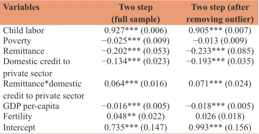
The estimated result indicated that poverty is negatively related to
child labor and is statistically significant at 1%. The sign doesn’t
change even after removing outliers, though not statistically
significant in the second instance, this invariably supported the
paradoxical wealth effect proposition as advanced by Bhalotra
and Heady (2003) which indicated that child labor use mostly
emerges from the richest households. That is to say those children in land rich households are more likely to work and attend school less compared to the children in land poor households. This phenomenon is referred to as wealth paradox. This may be accounted to the fact that greater majority of the children that engages in child labor activities in developing countries relates to agricultural sub-sector such as farms operated by families. Other control variable such as GDP per-capita expressed expected sign of being negatively relating to child labor prevalence, which means increase in per-capita GDP tends to reduce child labor prevalence
in the sample countries. The over identification test (Sargan test)
failed to reject the hypothesis that instruments are not correlated with the error terms of the structural equations. Similarly there exist no second order serial autocorrelation in the model.
6. CONCLUSION AND POLICY
RECOMMENDATIONS
The present study empirically analyzed the impact of poverty on the prevalence of child labor across 42 developing countries. The result revealed that poverty increased rather than decreased
Table 1: Descriptive statistics
Variables Observation Mean Standard
deviation Min Max Child labor 210 2.472 0.861 0.693 4.285
Poverty 210 4.043 1.131 0 5.094
Remittances 210 0.838 1.643 −4.044 3.215 Domestic credit
to private sector 210 3.436 0.502 2.396 4.506 Remittance*
domestic credit to private sector
210 2.992 5.711 −13.069 11.839
GDP per-capita 210 7.269 0.967 5.215 9.316
Fertility 210 1.083 0.456 0.336 2.026
GDP: Gross domestic product
Table 2: GMM estimation on the effect of poverty on child labor in selected developing countries
Variables Two step
(full sample) removing outlier)Two step (after Child labor 0.927*** (0.006) 0.905*** (0.007) Poverty −0.025*** (0.009) −0.013 (0.009) Remittance −0.202*** (0.053) −0.233*** (0.085) Domestic credit to
private sector −0.134*** (0.023) −0.193*** (0.035) Remittance*domestic
child labor prevalence in developing countries over the period
under review. The study justified the paradoxical wealth effect as advanced by Bhalotra and Heady, (2003). The implication is
that developing countries in their quest to eliminate child labor should institute proper legislation in order to address the child labor problem considering the fact that the richer the households are in selected developing countries, the more vulnerable they become to child labor syndrome. Which means poverty of parents is not the main stimulus of child labor prevalence in the selected developing countries.
Therefore, governments of the developing countries should institute legislations inform of banning child labor in an attempt to eliminate the syndrome from developing countries. This may be connected to the fact that greater proportion of child labor participation is in agricultural sub-sector, hence, the more land you possess, the higher the possibility of sending children to employment. Families that don’t have land possession may not be able to send their children to employment even if they wish doing so.
REFERENCES
Bhalotra, S., Heady, C. (2003), Child farm labor: The wealth paradox. The World Bank Economic Review, 17(2), 197-227.
Basu, K. (1998), Child labor: Cause, consequence, and cure, with remarks on international labor standards. Journal of Economic Literature, 37(3), 1083-1119.
Basu, K., Van, P. (1998), The economics of child labor. American Economic Review, 88(3), 412-27.
Basu, K., Das, S., Dutta, B. (2010), Child labor and household wealth: Theory and empirical evidence of an inverted-U. Journal of Development Economics, 91(1), 8-14.
Belsley, D., Kuh, E., Welsh, R. (1980), Regression Diagnostics. New York: Wiley.
Bhalotra, S., Heady, C. (2003), Child farm labor: The wealth paradox. The World Bank Economic Review, 17(2), 197-227.
Blunch, N.H., Verner, D. (2001), Revisiting the link between poverty and child labor: The Ghanaian experience. World Bank Policy Research Working Paper. p2488.
Dumas, C. (2007), Why do parents make their children work? A test of the poverty hypothesis in rural areas of Burkina Faso. Oxford Economic Papers, 59(2), 301-329.
Ebeke, C.H. (2012), The power of remittances on the international prevalence of child labor. Structural Change and Economic Dynamics, 23(4), 452-462.
IPEC-ILO. (2013), International Programme on the Elimination of Child Labour. Geneva: ILO.
Nkamleu, G.B. (2006), Poverty and child farm labor in Africa: Wealth paradox or bad Orthodoxy. African Journal of Economic Policy, 13(1), 1-24. Appendix A
APPENDIX A
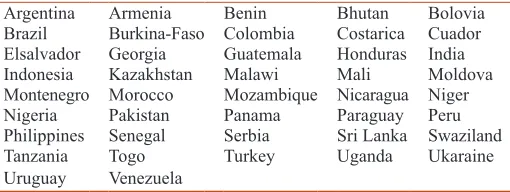
Table A1: List of sample countries for the study
Argentina Armenia Benin Bhutan Bolovia Brazil Burkina-Faso Colombia Costarica Cuador Elsalvador Georgia Guatemala Honduras India Indonesia Kazakhstan Malawi Mali Moldova Montenegro Morocco Mozambique Nicaragua Niger Nigeria Pakistan Panama Paraguay Peru Philippines Senegal Serbia Sri Lanka Swaziland
Tanzania Togo Turkey Uganda Ukaraine
Uruguay Venezuela
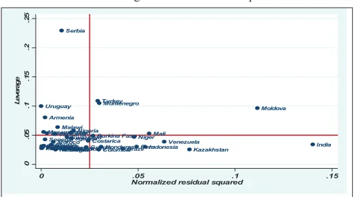
The study employs the use of DFITS test ignored to identify the countries that serves as outliers. The DFITS test which is given in the statistics as follows: DFITS =
r h
j j/ (
1
−
h
j)
where rj represent the residualas given byr e
j=
j/ (
s
( )j(
1
−
h
j) )
with s(j) and s referring to the root mean square errors (s) of the
regression equation with jth observation removed and h as the
leverage statistics (Belsley et al., 1980; Azman-Saini et al., 2010; Slesman, 2014). DFITS test identifies any observation which has
the high combination of leverage and residual, which according
to Belsley et al. (1980), is regarded as an outlier when DFITS
statistics is greater than 2 k n/ . k represent the number of regressors and n represent number of countries. Below is presented the result of DFITS test for the study (Figure B1).
The DFITS test result for full sample indicated that the following
countries are considered as outliers; Argentina (0.185), Ukraine (0.253)
lvr2plot, mlabel(country)
predict d1, cooksd
quietly generate cutoff = d1> 4/42 .list country d1 if cutoff +---+
| country d1 |
|---| 1. | Argentina .1846527 | 40. | Ukaraine .2528348 | +---+
APPENDIX B
Figure B1: Scatter plot of leverage versus residual squared for full sample
Argentina
ArmeniaBenin
BhutanBolivia Brazil Burkina Faso
ColombiaCostarica Ecuador ElsalvadorGeogia
Guatemala Honduras Indonesia Kazakhstan India Malawi
Mali Moldova Montenegro
Moroco Mozambique
Nicaragua
Niger Nigeria
Pakistan PanamaPhilippensParaguay Peru Senegal
Serbia
Srilanka SwazilandTanzaniaTogo
Turkey
uganda
Ukaraine
Uruguay
Venezuela
0
.0
5
.1
.1
5
.2
Le
ve
ra
ge
0 .05 .1 .15
Normalized residual squared
Figure B2: Scatter plot of leverage versus residual squared after removing outliers from the sample
Armenia
Benin Bhutan
Bolivia Brazil Burkina Faso
Colombia Costarica Ecuador Elsalvador Geogia
Guatemala Honduras Indonesia Kazakhstan India Malawi
Mali
Moldova Montenegro
Moroco Mozambique
Nicaragua
Niger Nigeria
PakistanPanamaPhilippensSenegalParaguay Peru Serbia
Srilanka Swaziland TanzaniaTogo
Turkey
uganda Uruguay
Venezuela
0
.0
5
.1
.1
5
.2
.2
5
Le
ve
ra
ge
0 .05 .1 .15